Multiple merging events in Abell 521

We present a detailed spatial and dynamical analysis of the central $\sim$ 2.2 ${{\rm h}_{75}}^{-1}$ Mpc region of the galaxy cluster Abell 521 (z=0.247), based on 238 spectra (of which 191 new measurements) obtained at the 3.6 m Telescope of the European Southern Observatory and at the Canada-France-Hawaii Telescope. From the analysis of the 125 galaxies that are confirmed members of the cluster, we derive a location (“mean” velocity) of ${\rm C}_{\rm BI}=74019^{+112}_{-125}$ km/s and detect a complex velocity distribution with high velocity scale (“dispersion”, ${\rm S}_{\rm BI}=1325^{+145}_{-100}$ km/s), but clear departure from a single Gaussian component. When excluding a possible background group of four galaxies, the velocity dispersion remains still large ($\sim 1200$ km/s). The general structure of the cluster follows a North-West/South-East direction, crossed by a perpendicular high density “ridge” of galaxies in the core region. The Northern region of the cluster is characterized by a lower velocity dispersion as compared to the whole cluster value; it hosts the BCG and a dynamically bound complex of galaxies, and it is associated with a group detected in X-ray (Arnaud et al. 2000). This region could be in a stage of pre-merger onto the main cluster. The small offset (${\sim}+250$ km/s) in the mean velocity of the northern region as compared to the whole cluster suggests that the merging occurs partly in the plane of the sky. These results, taken together with the fact that most of the clumps detected on the isodensity maps, as well as the early-type galaxies and the brightest ones (L$>{\rm L}^{*}$) are aligned, suggest that this North-West/South-East direction is the preferred one for the formation of this cluster. The central high dense region (“ridge”) shows a lower velocity location (${\rm C}_{\rm BI}\leavevmode\nobreak\ =\leavevmode\nobreak\ 73625^{+344}_{-350}$ km/s) and significantly higher scale ($1780^{+234}_{-142}$ km/s) as compared to the whole cluster values. This is due to the presence of a low-velocity group of galaxies with a high fraction of emission line objects. This can be explained in a scenario in which a merging of subclusters has recently occurred along the direction of the “ridge” with a significant component along the line of sight. The low-velocity group would then be a high-speed remnant of the collision which would have also triggered an episode of intense star formation responsible for the large fraction of late-type objects in this region.

1 Introduction

In the hierarchical model of structure formation, galaxy clusters are supposed to form by merging of units of smaller mass. Analysis of statistical samples of galaxy clusters have shown that a high percentage of clusters with substructures is detected even at low redshift, implying that clusters are still today undergoing the process of formation (Geller & Beers 1982, Dressler & Shectman 1988, Jones & Forman 1992). Moreover, quantifying precisely the amount of morphologically complex clusters allows one in principle to constrain directly the cosmological model through the density parameter $\Omega_{m}$ (Richstone et al. 1992, Mohr et al. 1995). This analysis is however hampered by the existing uncertainty in the rate at which substructure is erased (Kauffmann & White 1993, Lacey & Cole 1993). The second difficulty is that sub-clustering can affect the various quantities observable, such as the projected distribution of the galaxies and of the gas, the velocity distribution of the galaxies and the temperature structure of the gas, not necessarily at the same level, leading to sometimes different conclusions.

Detailed studies of individual complex galaxy clusters at different wavelengths is a complementary analysis which allows one to obtain details of the scenario of formation of these objects, and the physical processes necessary to explain the observed distribution (Flores et al. 2000, Donnelly et al. 2001, Mohr et al. 1996, Bardelli et al. 1998, Rose et al. 2002, Berrington et al. 2002, Czoske et al. 2002, Valtchanov et al. 2002). In this paper, we will concentrate on the dynamical analysis of the merging cluster Abell 521 which has been targeted for its outstanding properties.

Abell 521 is a rich (R=1) Abell cluster, first detected in X-ray with HEAO1 (Johnson et al. 1983, Kowalski et al. 1984). It was also suspected (Ulmer et al. 1985) to form a binary cluster together with its nearest neighbor on the sky, A518, but no clear evidence for gas interaction was found between the two clusters. Radio observations in the region of this cluster (Hanisch et al. 1985) have also shown a high fraction of radio sources with projected distances to the center compatible with these objects being cluster members. More recent data, both in X-ray and optical (Arnaud et al. 2000, Maurogordato et al. 2000) provided a more detailed analysis of the properties of the galaxies and gas distributions in this cluster. Imaging in X-ray (ROSAT/HRI) has shown a gas morphology with two peaks which can respectively be associated with a diffuse main cluster, and a compact less massive group in the northern region, suspected to be in pre-merger stage with the main cluster. The projected galaxy density distribution in the central 2.2 ${{\rm h}_{75}}^{-1}$ Mpc has a very anisotropic morphology, as it exhibits two high density filaments crossing in an X-shape structure at the barycentre of the cluster. A severe gas/galaxy segregation stands out. The brightest cluster galaxy is offset of the cluster barycentre, and lies in the region of the X-ray northern group. Multi-object spectroscopy at ESO/EFOSC2 and CFHT/MOS led to the determination of the mean redshift of the cluster, z=0.247, and of its velocity dispersion ${\rm S}_{\rm BI}=1386$ km/s as measured from 41 members. However, this very high value of the velocity dispersion could be affected by the presence of substructures. Its value is also high compared to the temperature of the X-ray gas measured with ASCA (T=6.3 KeV, Arnaud et al. 2000). These results imply that this cluster is undergoing strong dynamical evolution. This motivated new observations in order to better characterize the merging scenario, in particular through additional multi-object spectroscopy. A project of wide-field multicolor imaging in five bands is under progress, and will address the large scale environment of the cluster using photometric redshifts (Ferrari et al. in prep.). In this paper, we analyze in detail the velocity distribution within the central 2.2 ${{\rm h}_{75}}^{-1}$ Mpc of the cluster with new data obtained at the ESO 3.6 m telescope (191 new redshifts measured). Section 2 briefly describes the observations and the data processing techniques, as well as the level of completeness achieved. In Sect. 3, we perform a general analysis of the 1D velocity distribution, test for departures from an unimodal gaussian, and fit a partition in three velocity groups. In Sect. 4, correlations between the structures identified in velocity space and in projected coordinates have been looked for. Variations of dynamical properties with absolute luminosity, color, and spectral type have been addressed in Sect. 5. In Sect. 6, our new data are used to elaborate the more plausible scenario of occurrence of the various merging events within this particularly complex cluster. All numbers are expressed as a function of ${\rm h}_{75}$, the Hubble constant in units of 75 km/s/Mpc. We have used the $\Lambda$CDM model with $\Omega_{\rm m}=0.3$ and $\Omega_{\Lambda}=0.7$, then 1 arcmin corresponds to $\sim$0.217 ${{\rm h}_{75}}^{-1}$ Mpc in the following.

2 The data

2.1 Observations and data reduction

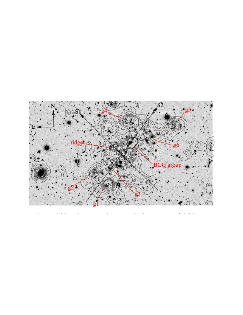
Figure 1: Central field (20’$\times$10’) of the cluster. In black, galaxy iso-density contours for B$<$27 and I$<20$; the lowest iso-density contour corresponds to 1$\sigma$ level above the mean density in the field, the contours are spaced by 0.5$\sigma$. Black circles correspond to the 125 galaxies of the cluster with spectral quality flag=1. The subgroups identified in the projected density map and the two main directions of the cluster (S1 and S2) have been shown.

New data have been obtained through a campaign of multi-object spectroscopy at the ESO 3.6 m telescope (3 nights in October 1999, and 2.5 nights in December 2000). We used the ESO Faint Object Spectrograph and Camera (EFOSC2) with grism#04, whose grating of 360 line ${\rm mm}^{-1}$ leads to a dispersion of 1.68 Å/pixel, and a wavelength coverage ranging from 4085 to 7520 Å. The detector used was the EFOSC2 CCD Loral/Lesser#40, with an image size of 2048 $\times$ 2048 (we made a 2 $\times$ 2 binning, in order to improve the signal to noise ratio), and a pixel size of 15 $\times$ 15 $\mu$m.

During the run of October 1999 we achieved a spectral resolution of FWHM$\sim$18.5 Å, while in the second run, as a smaller punching head was available ($1.35^{\prime\prime}$ instead of $1.8^{\prime\prime}$), the resolution was improved to FWHM$\sim$12.5 Å. The total integrated exposure time was 9000 s for each frame, split in at least two exposures to eliminate cosmic rays. After each science exposure, a Helium-Argon lamp exposure was systematically taken for wavelength calibration.

Data have been reduced with IRAF, using our automated package for multi-object spectroscopy based on the task “apall”. Radial velocities were determined using the cross-correlation technique (Tonry & Davis, 1981) implemented in the RVSAO package (developed at the Smithsonian Astrophysical Observatory) with radial velocities standards obtained from the observations of late-type stars. We have obtained 191 new spectra. Among these, 29 are stars, while 109 are identified as galaxy spectra with a signal to noise ratio sufficient to obtain radial velocity measurement with a parameter R of Tonry & Davis greater than 3. The remaining 53 objects have a poor velocity determination.

We list in Table 10 our new velocity measurements. The columns read as follows: Col. 1: identification number of each target galaxy; Col. 2: run of observations (October 1999=ESO1, December 2000=ESO2); Cols. 3 and 4: right ascension and declination (J2000.0) of the target galaxy; Cols. 5 and 6: best estimate of the radial velocity and associated error from the cross-correlation technique (those values have been set to “-2” if the object is a star and to “-1” if we have no redshift information); Col. 7: a quality flag for the redshift determination: 1=good determination (R $\geq$ 3), 2=uncertain determination, 3=very poor determination, 4=failed spectra, Col. 8: a listing of detected emission lines.

Figure 2: I-band magnitude distributions of the galaxies of our spectroscopic sample (187 objects - solid line), of all the galaxies with good velocity determination (141 - dot), and, among them, of those belonging to A521 (113 - dash).

Figure 3: Velocity completeness for different cuts in I-band magnitude in the central $10{\times}10\leavevmode\nobreak\ {\rm arcmin}^{2}$ field covered by spectroscopy.

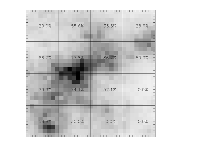
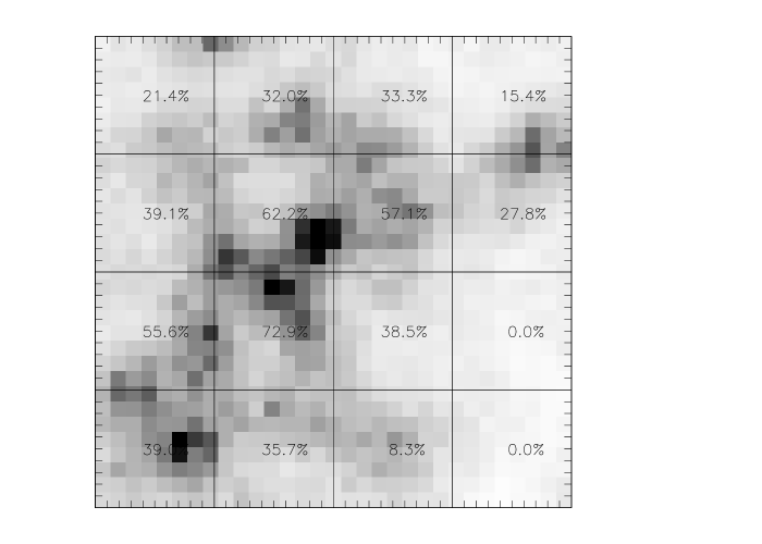
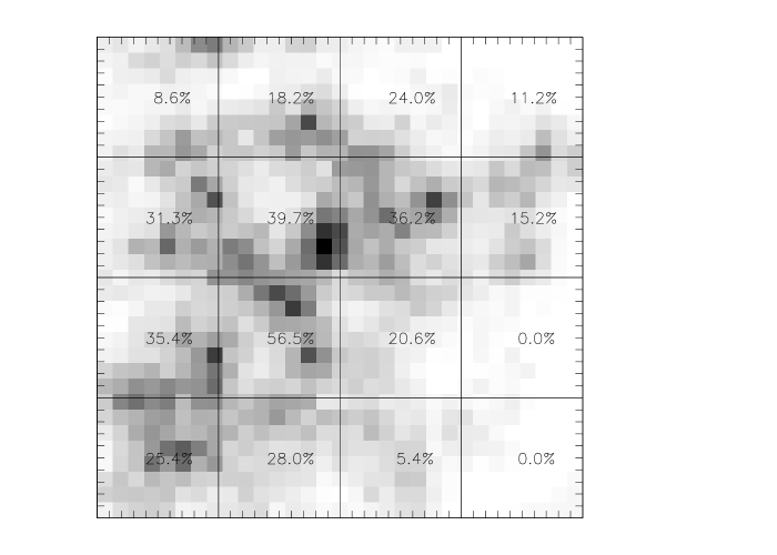
Figure 4: Completeness factor is superimposed to the isodensity maps in the field selected for spectroscopy (10’$\times$10’). Each cell of the grid covers 2.5’$\times$2.5’. Different magnitude cuts have been considered; from top to bottom: I$<$19, I$<$20, I$<$21.

2.2 The spectroscopic sample

In the following analysis, the new set of spectroscopic data presented above has been combined to our original sample (Maurogordato et al. 2000, 47 objects added to our new catalogue) resulting in a sample of 209 galaxies and 29 stars.

B- and I-band imaging (CFH12k) taken as part of our multicolor imaging program were used to build a color catalogue in the central region of the cluster surveyed by spectroscopy. This allowed to associate B- and I-band magnitudes for most galaxies of the spectroscopic sample (187), except for 22 objects located in the gaps between the chips of the camera or strongly blended. Fig. 1 displays the central field of the cluster, where galaxies with secure redshift determination have been circled. The isodensity map of the projected distribution of galaxies with I-band magnitude I$<$20 is also displayed (derived using the Dressler algorithm; Dressler 1980). The preferential directions S1 and S2 observed in Arnaud et al. 2000 are indicated. The density structures detected at more than $5\sigma$ level are also indicated: six groups called g1 to g6, a group around the BCG, and the so-called “ridge” structure corresponding to S1.

In Fig. 2 we have plotted the I-band magnitude distributions of: the galaxies of our magnitude/velocity sample (187), those with a very good redshift determination (141), and, among them, those belonging to the cluster (113). In Fig. 3 we show the ratio of the number of objects with measured velocities to the total number of galaxies detected within the central $10{\times}10\leavevmode\nobreak\ {\rm arcmin}^{2}$ of the field as a function of the I-band magnitude. We reach a general level of completeness for spectroscopy of 50% at ${\rm I}_{\rm AB}=19.5$, which drops at 30% at ${\rm I}_{\rm AB}=20.5$. However, these values are strongly affected by several incomplete fields at the periphery of the cluster, as the central dense regions of the cluster have been much better sampled. In fact, we have divided the spectroscopic field in $2.5{\times}2.5\leavevmode\nobreak\ {\rm arcmin}^{2}$ cells (Fig. 4), and measured the degree of completeness in each cell for three different cuts in I magnitude (${\rm I}_{\rm AB}=19,20,21$). The obtained values are shown in each cell of the corresponding isodensity maps. At ${\rm I}_{\rm AB}=19$, we have an excellent velocity sampling (${\sim}75{\div}80$% completeness) in the North-West/South-East main structure of the cluster, which drops at ${\sim}60$% at ${\rm I}_{\rm AB}=20$, and at ${\sim}40$% at ${\rm I}_{\rm AB}=21$.

3 The velocity distribution

3.1 Global analysis of the velocity distribution

We have analyzed the general behavior of the velocity distribution with the ROSTAT package (Beers et al. 1990). For this purpose, and in all the following analysis, we have used only the 125 objects with quality flag=1 (secure redshift) in our dataset; their velocity histogram is shown in Fig. 5.

In the case of large number of redshifts ($100{\leq}{\rm n}{\leq}200$) as in our situation, the best choice to estimate location (“mean” velocity) and scale (velocity “dispersion”) is the biweight estimator (Beers et al. 1990), as it provides the best combination of resistance and efficiency across the possible contaminations of a simple gaussian distribution. We find a location ${\rm C}_{\rm BI}=74019^{+112}_{-125}$ km/s and a scale ${\rm S}_{\rm BI}=1325^{+145}_{-100}$ km/s. These results are in good agreement with those obtained from the analysis of our former sample of 41 galaxies (Maurogordato et al. 2000), and confirm the apparently high value of the velocity dispersion in this cluster.

Figure 5: Velocity histogram within Abell 521 obtained from the 125 Q.F.=1 members of the cluster, with a binning of 500 km/s. A gaussian function with the velocity distribution derived with ROSTAT is superimposed.

Figure 6: Stripe density plot of radial velocities for the 125 members of Abell 521.

Figure 7: Same as Fig. 5, but now the best fit Gaussians found by KMM for a three group partition is superimposed and we have used a binning of 500 km/s.

Figure 8: Projected coordinates of the galaxies assigned to the KMM partition. From top to bottom, KMM-A, KMM-B, KMM-C. The subgroups of the cluster identified by the isodensity contours in Figs. 1 and 10 have been schematically represented (in next figures too).

We have also analyzed the higher moments of the distribution, in order to look for possible deviations from gaussianity that could provide important signature of dynamical processes. For all the following tests the null hypothesis is that the velocity distribution is a single Gaussian. The traditionally used shape estimators are kurtosis and skewness; in addition, we have computed the asymmetry and tail indices (AI and TI), which also measure the shape of a distribution, but are based on the order statistics of the dataset instead of its moments (Bird & Beers, 1993). By definition, skewness, kurtosis and AI are equal to 0 for a gaussian dish, while TI to 1. In Table 1 we present the results; significance levels have been estimated from Table 2 in Bird & Beers 1993. While the values obtained for skewness and AI cannot allow to reject the Gaussian hypothesis (significance level $>$ 10%), both kurtosis and TI indicate departure from a Gaussian distribution at better than 10% significance level (Beers et al. 1991). This indicates that the dataset has more weight in the tails than a Gaussian of the same dispersion.

As departure from normality and high values of velocity dispersion can result from a mixing of several velocity distributions of smaller velocity dispersion with different locations, we have investigated various tests for the existence of substructure in the cluster velocity distribution.

Table 1: 1D substructure indicators for the 125 objects with quality flag=1 in our dataset

Indicator	Value	Significance
AI	0.470	$\leq$0.20
TI	1.113	$\leq$0.10
Skewness	0.087	$>$0.20
Kurtosis	0.779	$\leq$0.05

We have therefore addressed the presence of gaps which can be a signature of sub-clustering (Beers et al. 1991). Five significant gaps in the ordered velocity dataset were detected. Fig. 6 shows the stripe density plots of radial velocities of the 125 cluster galaxies and we have indicated the gap positions with an arrow, while in Table 2 one can find the velocity of the object preceding the gap, the normalized size (i.e., the “importance”) of the gap itself, and the probability of finding a normalized gap of this size and with the same position in a normal distribution. Two very significant gaps are detected respectively at $\sim$ 76740 km/s (probability lower than 1.4%) and $\sim$ 72150 km/s (probability lower than 0.2%).

Table 2: Weighted gaps in the data

Velocity [km/s]	Size	Significance
73455.4	2.298	0.030
75243.4	2.323	0.030
73704.0	2.454	0.030
76738.1	2.577	0.014
72150.0	3.089	0.002

In addition, 9 of the 13 one-dimensional statistical tests of gaussianity performed by ROSTAT exclude the hypothesis of a single Gaussian distribution at better than 10% significance level (see Table 3). Among them, the Dip test is particularly indicative (Hartigan & Hartigan 1985). This tool tests the hypothesis that a sample is drawn from a unimodal, not necessarily Gaussian parent population. In the present case it rejects the unimodal hypothesis at a significance level better than 5%, confirming our previous results.

Table 3: 1-D statistical tests performed in ROSTAT package that exclude the hypothesis of a single gaussian distribution. In Cols. 1 and 2 we report the name and the value of the statistics, while Col. 3 indicate their significance levels.

Statistical Test	Value	Significance
a	0.743	$\leq$0.10
W	0.969	0.08
B2	3.779	0.04
DIP	0.023	$\leq$0.05
KS	0.873	0.10
V	1.707	0.01
${\rm W}^{2}$	0.162	0.02
${\rm U}^{2}$	0.162	0.01
${\rm A}^{2}$	0.989	0.01

3.2 Partitioning the distribution in velocity space

In order to separate possible velocity groups within our velocity dataset we have used the KMM mixture modeling algorithm of McLachlan & Basford (1988). This method has been shown to be very useful for detecting bimodality in astronomical datasets (Ashman and Bird 1994), and can even be applied to detect multimodality. One of the major uncertainties however is the best choice of the number of groups for the partition. Given the appearance of the velocity histogram and of the strip density plot, and the presence of two highly significant gaps, we have chosen as a first guess to fit three velocity groups around the mean velocities 70000, 74000 and 78500 km/s. The KMM algorithm then fits a 3-group partition from this guess and optimizes the mean velocity for each group. However, in the case of a multimodal partition, the significance level is not determined accurately by the algorithm. The estimated P-value of 3 % suggests a strong rejection of the null hypothesis (unimodal gaussian distribution) but has to be taken only as a guideline. The low-velocity group A is best fitted by a Gaussian with parameters: ${\rm C}_{\rm BI}=71127^{+207}_{-199}$ km/s and ${\rm S}_{\rm BI}=678^{+88}_{-69}$ km/s (17 objects). The major group B (103 objects) is found with ${\rm C}_{\rm BI}=74249^{+88}_{-90}$ km/s and ${\rm S}_{\rm BI}=879^{+61}_{-55}$ km/s. At the high velocity tail, 5 galaxies are found, with location ${\rm C}_{\rm BI}=78416^{+312}_{-184}$ km/s, populating group C. The three gaussians corresponding to these partitions are displayed in Fig. 7.

We present in Fig. 8 the projected positions of the galaxies assigned to the three partitions. The position of the main overdensities emerged in the projected density maps are also displayed for an easier reading. Galaxies in KMM-B are following the cross-like general pattern of the cluster. Half of the galaxies in KMM-A are located in the central ridge. Galaxies belonging to KMM-C are all located in the South-East region of the cluster. We have also tried partitions with a higher number of groups (respectively 4 and 5) which also show strong rejection of the unimodal hypothesis. However, as suggested by Ashman and Bird 1994, we have followed the Occam’s razor and selected the partition with the smaller number of groups (tri-partition).

4 Combined analysis of sub-clustering in velocity/2D space

4.1 Tomography of Abell 521

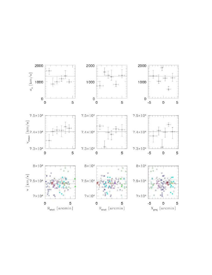
Figure 9: Left (from bottom to top): radial velocities of the 125 galaxies of our spectroscopic catalogue, and velocity location and scale of concentric shells with a fixed number of objects (20), centered on the optical barycentre of the cluster. Center: as before, but the new origin of the x-axis is the BCG position. Right: as before, but ${\rm X}_{\rm proj}$ is the projected coordinate along the main axis of the cluster (NW/SE) and the center position is again on the optical barycentre of the cluster. Continuous lines represent the whole sample velocity scale (top) and location (mean and bottom). Dashed lines (bottom) indicate the [${\bar{\rm v}}-\sigma_{\rm v},{\bar{\rm v}}+\sigma_{\rm v}$] interval. Different colors correspond to the different subgroups detected on the isodensity map: red open squares: BCG group -  blue open squares: ridge region -  cyan open squares: clump g1 -  green open squares: g2 -  purple open squares: g3 -  yellow open squares: g4 -  green full squares: g5 -  cyan full squares: g6 -  black open squares: remaining objects

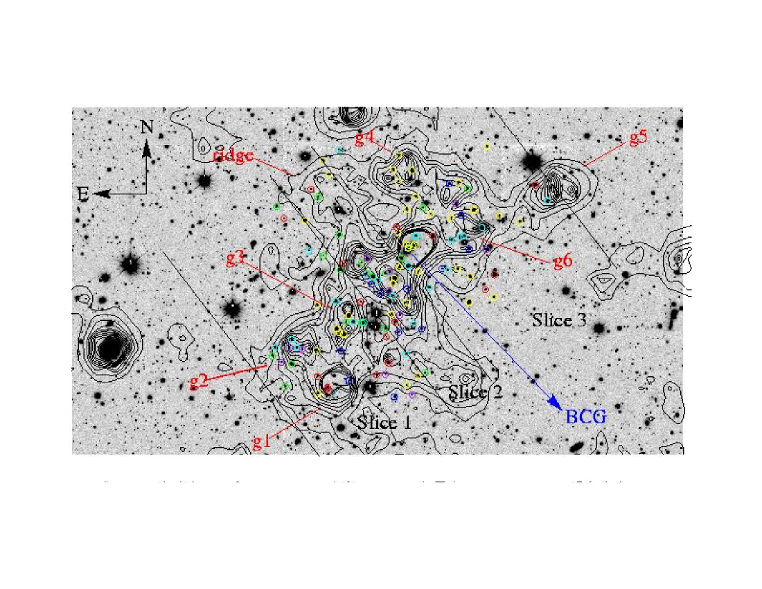
Figure 10: In black, galaxy iso-density contours for B$<$27 and I$<$20; the lowest iso-density contour corresponds to 1$\sigma$ level above the mean density in the field, the contours are spaced by 0.5$\sigma$. The division in 3 slices has been shown. Circles correspond to the galaxies in our high quality velocity dataset; different colors correspond to different ranges in radial velocity: blue: ${\rm v}_{r}=69000{\div}72000$ -  green: ${\rm v}_{r}=72000{\div}73000$ -  cyan: ${\rm v}_{r}=73000{\div}74000$ -  yellow: ${\rm v}_{r}=74000{\div}75000$ -  red: ${\rm v}_{r}=75000{\div}76000$ purple: ${\rm v}_{r}=76000{\div}80000$

As indicated by the moments analysis, the tails of the velocity distribution appear to be widely populated, suggesting the presence of interlopers. Moreover, the analysis of the number density maps of the cluster (Arnaud et al. 2000 and Fig. 1 of the present paper) shows a complex structure, with six groups in projected coordinates (g1 to g6) along the main SW/NE direction of the cluster, a group around the BCG and a high density ridge in the direction perpendicular to the main axis of the cluster.

In Fig. 9, the values of the radial velocities (bottom), the mean radial velocities (middle), and the velocity dispersions (top) are plotted as a function of an angular radius; velocity location and scale have been computed in concentric shells with a fixed number of objects (20), in order to have comparable statistics. Different colors in the velocity vs. radius plots have been used to visualize the different groups identified on the isodensity map.

For the left panels, the center is taken at the position of the main X-ray cluster (Arnaud et al. 2000), which roughly coincides with the barycentre of the galaxy distribution. For the plots of the central column the origin is centered on the BCG position, while in the the right panels we used the projected coordinate along the cluster main axis S2 (North-West/South-East). Negative values correspond to the South-East extremity of the cluster, zero to the center, and positive values to the North-West extent.

In Fig. 10, galaxies have been circled with different colors corresponding to different velocity bins. Fig. 9 and Fig. 10 can then be analyzed together to understand the variation of the velocity distribution in the field. The galaxies belonging to the region of the “ridge” S1, centered on the barycentre position and extending perpendicularly to the main axis S2, are color-encoded as blue open squares in Fig. 9. For this particular region, we obtain systematically a lower mean velocity and a higher dispersion than for the whole cluster. This is particularly apparent in Fig. 9 top and medium, right panels. This region consists of several clumps in projected density map, but galaxies in the whole velocity range [70000-78000] km/s populate the various clumps. However, it is the large number of low velocity objects that lowers the value of location in this region as compared to that obtained for the whole cluster.

At $\sim$ 1.5 arcmin from the barycentre of the cluster, in the North-East direction, we find a compact region of galaxies at similar velocities corresponding to the BCG region (galaxies color-encoded as red squares in the bottom panels of Fig. 9), which shows a significantly lower velocity dispersion and a slightly higher value of the mean velocity (top and medium panels of Fig. 9).

A high velocity group of four galaxies ($\sim$ 78500 km/s) is detected at large radius ($\sim$ 4 arcmin) from the barycentre of the cluster (bottom panel of Fig. 9), with a gap in velocity of more than 1500 km/s as compared to others galaxies at the same radius. Thus, these objects are likely to be unbound to the cluster; they are located in the South-East extremity of the cluster (bottom, right panel of Fig. 9), and three of them in the region defined as g2 (green open squares in Fig. 9). This latter is the result of the superimposition along the line of sight of these three high velocity galaxies and a concentration of objects in the velocity range ([72000-74000] km/s).

Several other clumps have a more homogeneous velocity composition: g1 (cyan open squares in Fig. 9), g3 (purple open squares in Fig. 9, and g4 ( yellow open squares in Fig. 9); g1 is mainly populated with galaxies in the [74000-76000] km/s velocity range, while the greatest part of objects in g3 have velocity in the [74000-75000] km/s bin. In particular, as one can see comparing the first and fifth bins of the central, top panels of Fig. 9, g3 has a mean velocity and velocity dispersion quite close to the value of the BCG group. The North-East g4 clump also shows a mean velocity location comparable to the BCG region, and a very small value of velocity dispersion.

Unfortunately, the number of measured radial velocities within the previous mentioned substructures is not always large enough to obtain meaningful dynamical information for each of them; we have thus divided the cluster into three regions with a number of objects sufficient to derive stable estimators of location and scale and to get enough statistics in velocity histograms without degrading too much the binning. These regions have been defined as three slices perpendicular to the main direction of the cluster (see Fig. 10). This choice has been motivated by the following reasons: first of all we wish to test separately the velocity distribution within the high density ridge S1 perpendicular to the direction of the main cluster S2, which was shown in previous analysis to be of specific interest. We therefore design the central slice (2) to include it. We also want to investigate the possible differences in velocity distribution between the North-West and South-East regions suggested in Fig. 9. The southern slice (1) includes the groups g1, g2 and g3; the northern slices (3) includes both the BCG region as well as the northern extensions embedding g4, g5 and g6 subgroups. In Fig. 11 the velocity distributions for each slice are shown; the corresponding values for velocity location and scale have been reported in Table 4.

In the southern region (slice 1), the mean velocity of the main structure, obtained when excluding the four high velocity galaxies, is ${\rm C}_{\rm BI}\leavevmode\nobreak\ =\leavevmode\nobreak\ 73886^{+186}_{185}$ km/s, and its scale is ${\rm S}_{\rm BI}\leavevmode\nobreak\ =\leavevmode\nobreak\ 1117^{+150}_{-86}$ km/s. The bimodal appearance of the main structure histogram motivated us to try a KMM partitioning of the distribution. A very good agreement was found (0.929 significance level) for a fit by two gaussians centered respectively at 73070 km/s and 75140 km/s, and with velocity dispersions of ${\rm S}_{\rm BI}\leavevmode\nobreak\ =\leavevmode\nobreak\ 570^{+89}_{-52}$ km/s and ${\rm S}_{\rm BI}\leavevmode\nobreak\ =\leavevmode\nobreak\ 498^{+87}_{-40}$ km/s. This indicates that in the region there is probably a mix of two kinematically distinct populations in addition to the high velocity group, and reflects the previous mentioned difference in velocity distribution within the clumps g1 and g3 with respect to g2.

In slice 2, corresponding to the ridge region, the velocity distribution shows a very dispersed boxy shape, with a velocity dispersion reaching the very large value of $1780^{+234}_{-142}$ km/s, in good agreement with previous values by Maurogordato et al. 2000. In agreement with previous results, the location of the central slice is the lowest one (${\rm C}_{\rm BI}\leavevmode\nobreak\ =\leavevmode\nobreak\ 73625^{+344}_{-350}$ km/s).

The northern region (slice 3) shows a higher location than the previous slices, ${\rm C}_{\rm BI}\leavevmode\nobreak\ =\leavevmode\nobreak\ 74300^{+110}_{-104}$ km/s, which is comparable to the velocity of the BCG ($74357{\pm}44$ km/s), and a lower velocity dispersion (${\rm S}_{\rm BI}\leavevmode\nobreak\ =\leavevmode\nobreak\ 839^{+216}_{-134}$ km/s). The shape of the distribution is symmetrical, although few galaxies are still present in the low velocity tail. We have addressed the dynamics of the region immediately surrounding the BCG; this galaxy has a complex structure, with a series of bright knots embedded in a lower density arclike structure at 24 ${{\rm h}_{75}}^{-1}$ kpc of its center (Maurogordato et al. 1996, Maurogordato et al. 2000). We have measured the redshifts of the four bright knots in the arclike structure (see Table 5), showing that these objects belong to the cluster and are not gravitationally lensed background objects. The central location in a $\sim$ 240 ${{\rm h}_{75}}^{-1}$ kpc region around the BCG (ten objects with measured velocities including the BCG and its multiple nuclei) is ${\rm C}_{\rm BI}\leavevmode\nobreak\ =\leavevmode\nobreak\ 74340^{+40}_{-102}$ km/s. This values is very close to the BCG radial velocity (74357$\pm$44 km/s); the velocity scale is very low, $256^{+82}_{-133}$ km/s, and of the same order as the BCG internal velocity dispersion, 368$\pm$463 km/s (Maurogordato et al. 2000) strongly suggesting it is bound to the BCG.

When comparing the velocity distribution of the three slices, the northern region clearly shows a higher location and a lower velocity dispersion than the other regions, while a very high velocity dispersion is observed within the central ridge. These results confirm the trends that emerged in the velocity profiles in Fig. 9.

Table 4: Velocity distribution properties of the various subsamples of A521 galaxies

Subsample	Galaxy nb.	${\rm C}_{\rm BI}$	${\rm S}_{\rm BI}$
		[km/s]	[km/s]
Whole sample	125	$74019^{+112}_{-125}$	$1325^{+145}_{-100}$
KMM-A	17	$71127^{+207}_{-199}$	$678^{+88}_{-69}$
KMM-B	103	$74249^{+88}_{-90}$	$879^{+61}_{-55}$
KMM-C	5	$78416^{+312}_{-184}$	-
Non-emission line	110	$74166^{+96}_{-112}$	$1087^{+117}_{-88}$
galaxies
Emission line	15	$72390^{+727}_{-923}$	$2250^{+752}_{-384}$
galaxies
Early	72	$74083^{+121}_{-145}$	$1105^{+135}_{-95}$
Late	41	$73402^{+258}_{-278}$	$1723^{+272}_{-170}$
Bright	9	$74321^{+118}_{-193}$	$491^{+265}_{-243}$
(${\rm I}_{\rm AB}<{{\rm I}_{\rm AB}}^{*}$)
Intermediate	76	$74000^{+144}_{-164}$	$1331^{+156}_{-150}$
(${{\rm I}_{\rm AB}}^{*}<{\rm I}_{\rm AB}<{{\rm I}_{\rm AB}}^{*}$+2)
Faint	28	$73515^{+268}_{-311}$	$1635^{+449}_{-232}$
(${\rm I}_{\rm AB}>{{\rm I}_{\rm AB}}^{*}$+2)
Slice 1	44	$74037^{+233}_{-256}$	$1454^{+266}_{-180}$
Slice 1 without	40	$73886^{+186}_{-185}$	$1117^{+150}_{-86}$
the background group
Slice 2	30	$73625^{+344}_{-350}$	$1780^{+234}_{-142}$
Slice 3	51	$74298^{+110}_{-104}$	$839^{+216}_{-134}$

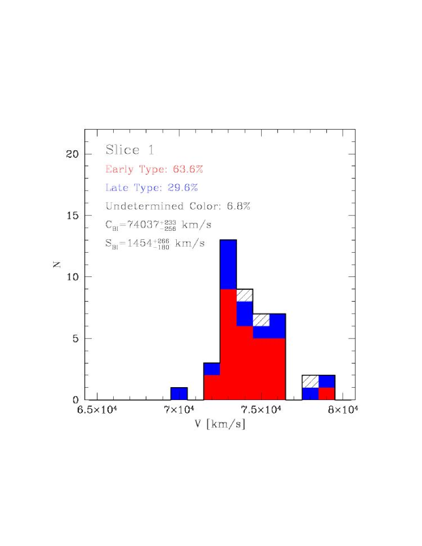
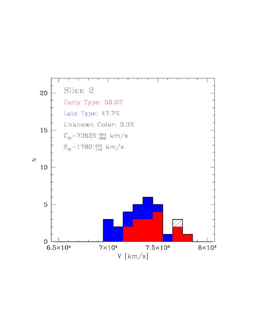
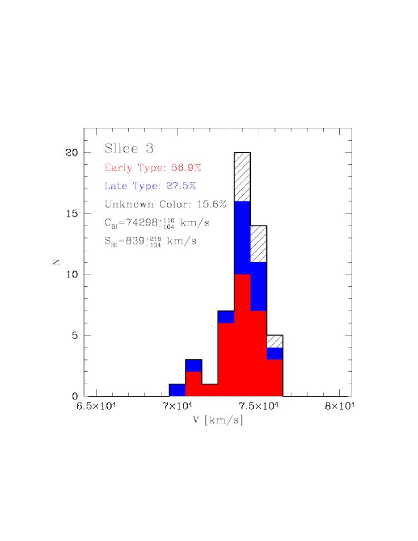
Figure 11: Velocity distributions of the three slices of Fig. 10; the contribution due to different morphological types has been shown using different colors (early: red, late: blue, undetermined color objects: black shading). A binning of 1000 km/s has been used. Velocity location and scale found with ROSTAT are also shown.

Table 5: Radial velocities of the four blobs embedded in the arclike structure at 24 ${{\rm h}_{75}}^{-1}$ kpc of the BCG center. The names of the blobs refer to Maurogordato et al. 2000, Fig. 8.

Blob	Radial Velocity(km/s)	Error on Velocity(km/s)
B	74340	100
C	74341	80
D	74325	52
E	74205	106

Figure 12: Projected positions of the galaxies in our spectroscopic sample, represented by circles with dimensions weighted by the estimators of Dressler & Shectman 1988 (${\Delta}$, top panel) and Girardi et al.  1997 (${\delta}_{\rm V}$, middle panel , and ${\delta}_{\rm S}$, bottom panel). In the top panel, concentrations of large circles indicate a correlated spatial and kinematical variation. In the middle panel, strong deviations of the local velocity as compared to the global one, while in the bottom panel, a low value of the local velocity dispersion as compared to the mean one. Crosses correspond to circles larger than the box (see text for details).

4.2 Kinematical indicators of sub-clustering

Our previous analysis has clearly shown the presence of sub-clustering in the projected density distribution and the departure from gaussianity of the velocity distribution, indicating that the system has not yet reached equilibrium. As a second step, we have performed a more systematic search of sub-structures by addressing directly correlated deviations in position and velocity distributions. We have applied several classical methods that quantify the amount of substructures in galaxy clusters using positions and velocities.

In Table 6 we list the actual values for $\Delta$ (Dressler & Shectman, 1988), $\epsilon$ (Bird, 1994), and $\alpha$ (West & Bothun, 1990) parameters and the significance of the corresponding tests, obtained through the bootstrap technique and by normalizing with 1000 Monte Carlo simulations.

Table 6: 3-D substructure indicators for the sample of 125 objects with quality flag=1 in our dataset

Indicator	Value	Significance
$\Delta$	164.8	0.080
$\epsilon$	${1.91}{\times}{10}^{+27}\leavevmode\nobreak\ {\rm kg}$	0.217
$\alpha$	0.183 ${{\rm h}_{75}}^{-1}$ Mpc	0.381

Assuming that these tests reject the null hypothesis if the significance level is less than 10%, only the $\Delta$ test finds evidences of subclustering at a high confidence level. This result is further investigated by using the kinematical estimators introduced by Girardi et al. (1997), which take into account separately the departures of the local mean (${\delta}_{\rm V}$) and dispersion (${\delta}_{\rm S}$) from the global measurements for the whole cluster. Low values of local velocity dispersion will give high values of ${\delta}_{\rm S}$, while ${\delta}_{\rm V}$ will be high in case of strong departures (i.e. more than one $\sigma$) of the local mean velocity with respect to the global mean. In Fig. 12, each galaxy is represented by a circle whose diameter is proportional to $e^{{\Delta}}$ (top panel), $e^{{\delta}_{\rm V}}$ (middle panel) and $e^{{\delta}_{\rm S}}$ (bottom panel). The top panel shows several areas with many large circles, which indicate correlated spatial and kinematic variations. In the middle panel, very large circles are present in the South-East region of the cluster, corresponding to the group of background galaxies detected in previous sections. One can also note several large circles in the ridge region, corresponding to the presence of the previously detected low velocity group. Moreover, in the bottom panel, we detect three clumps in which the velocity dispersion is effectively low; one is in the South-East region and corresponds to the structure identified as g3 in our iso-density maps, while the second is centered on the BCG complex. The third clump consists of a group of four galaxies in the g4 region; it has such a low local velocity dispersion that the corresponding $e^{{\delta}_{\rm S}}$ values are larger than the box size of Fig. 12. Therefore, we have represented these objects with circles of diameter equal to their $\delta_{\rm S}$ parameters, and we have indicated their projected positions with crosses. Their radial velocities are in the range [74200-74500] km/s, as can clearly be seen in Fig. 9, where the four galaxies are represented by yellow squares. We also note that in the region of the “ridge” and in the extreme South-East region, the dimension of the circles is the smallest, indicating in these regions the highest values of the velocity dispersion are reached.

Figure 13: Substructure analysis by the h-tree method: the map in projected coordinates is shown, with different symbols corresponding to the different groups identified.

We have also applied the algorithm developed by Serna & Gerbal (1996) which identifies subclusters on the basis of dynamical arguments. It uses the hierarchical clustering algorithm to associate galaxies according to their relative binding energies. Fig. 13 shows the map in projected coordinates visualizing the groups resulting from the substructure analysis at the various levels. At the first level, the algorithm separates the data into the main cluster G1 of 120 objects (open circles + stars) with ${\rm v}_{mean}=73835$ km/s and $\sigma=1204$ km/s, and a high velocity set of 5 objects G2 (large filled points) in the southern region, with ${\rm v}_{mean}=78418$ km/s and $\sigma=500$ km/s, previously identified as KMM-C. The algorithm then splits again the main cluster G1 in two components of very different mass ratios: the main one G11 (93 objects, open circles) with a mean velocity similar to the value obtained for G1 , but now a velocity dispersion greatly reduced ($\sigma=940$ km/s), and a low mass group G12 of five objects at higher velocity (75730 km/s) plotted as stars in the southern region. These objects were already detected in the analysis of slice 1, as a possible higher velocity population of the southern region. At the last level of structure identification, the algorithm finds out two significant groups: the first one at North (G111), corresponding to the region surrounding the BCG galaxy (squares), at a slightly higher mean velocity than the mean component (74290 km/s) and presenting a low value of the velocity dispersion (442 km/s), and a compact group southern of the ridge (circles), corresponding to g3 in previous Sects. The energy levels of the various groups are also provided (not displayed): the deepest energy levels at the bottom of the energy well corresponds to the BCG complex. The lower level is occupied by the BCG itself associated to blob A, joining with the three other blobs C, D and E (see Table 5) at a slightly higher level. Associating to the BCG complex various galaxy pairs at low energy levels results into a bound central group around the BCG galaxy. It is interesting to note that the BCG group and g3 are detected both by the dynamical estimator of Girardi et al. 1997, and by the ${\rm h}_{\rm tree}$ algorithm.

4.3 Dynamics of the groups

As seen before, several groups are revealed from the sub-structure analysis. We have then performed the gravitational bound check as in the two-body problem (Beers, Geller and Huchra 1982):

$${{\rm V}_{r}}^{2}{\rm R}_{p}\leavevmode\nobreak\ \leq\leavevmode\nobreak\ 2\leavevmode\nobreak\ {\rm G}\leavevmode\nobreak\ {\rm M}\leavevmode\nobreak\ {\rm sin}^{2}{\alpha}\leavevmode\nobreak\ {\rm cos}{\alpha},$$ (1)

where ${\rm V}_{r}$ is the relative line-of-sight velocity of the two considered clumps, ${\rm R}_{p}$ is the projected separation of the clump centers, $\alpha$ is the projected angle measured from the sky plane, and M is the total mass of the system.

In a first step, we have applied it to the groups G1 and G2 previously defined by the h-tree method. The result is displayed in Fig. 14, which shows that the system is unbound for nearly all values of the projection angle $\alpha$. We have then eliminated the group G2 from the analysis as a background system of galaxies, and tested if the group G111 (corresponding to the system surrounding the BCG) and the group G112 (corresponding to g3) are bound to the remaining cluster. We considered each time a two-body problem, with one system being the tested group, and the other the remaining cluster. It results that the groups G111 and G112 are bound to the cluster for nearly all values of the projection angle $\alpha$ (4 to 90 degrees).

Table 7: Properties of the significant groups from the ${\rm h}_{\rm tree}$ analysis

group	${\rm v}_{\rm mean}$	$\sigma$	${\rm M}_{\rm vir}$	${\rm N}_{gal}$
	[km/s]	[km/s]	$(10^{15}M{\odot})$
main	74018	1386	1.96	125
G1	73835	1204	1.64	120
G2	78418	504	0.2	5
G11	73965	930	1.1	93
G12	75730	121	0.006	5
G111	74290	442	0.045	12
G112	74068	574	0.063	7

Figure 14: Boundary between the bound and unbound orbits for the main cluster G1 and the high velocity system G2. The domain left of the curve corresponds to bound orbits, while the right part to unbound ones. The vertical line corresponds to the velocity difference between the mean location of the two groups. The corresponding 68% confidence region is shown with the cross-hatching.

5 Variation of dynamical properties with color and luminosity

In this Sect. we use the color information to define early and late type galaxy subsamples, using the result that the bulk of early-type galaxies in all rich clusters usually lie along a linear color-magnitude relation. This so called “red sequence” has been interpreted as a clear indication that all rich clusters contain a core population of passively, evolving elliptical galaxies, coeval and formed at high redshift (Ellis et al. 1997, Kodama et al. 1999, Gladders et al. 1998). In Fig. 15 the (B-I) versus I color-magnitude diagram (CMD) is shown for the objects in a field of $15{\times}15\leavevmode\nobreak\ {\rm arcmin}^{2}$ (${\sim}3.25{\times}3.25\leavevmode\nobreak\ {{\rm h}_{75}}^{-2}\leavevmode\nobreak\ {\rm Mpc}^{2}$) centered on the optical barycentre of the cluster.

Due to the fact that we have no magnitude information for 12 of the 125 objects of A521, our velocity/magnitude catalogue is made up of 113 galaxies.

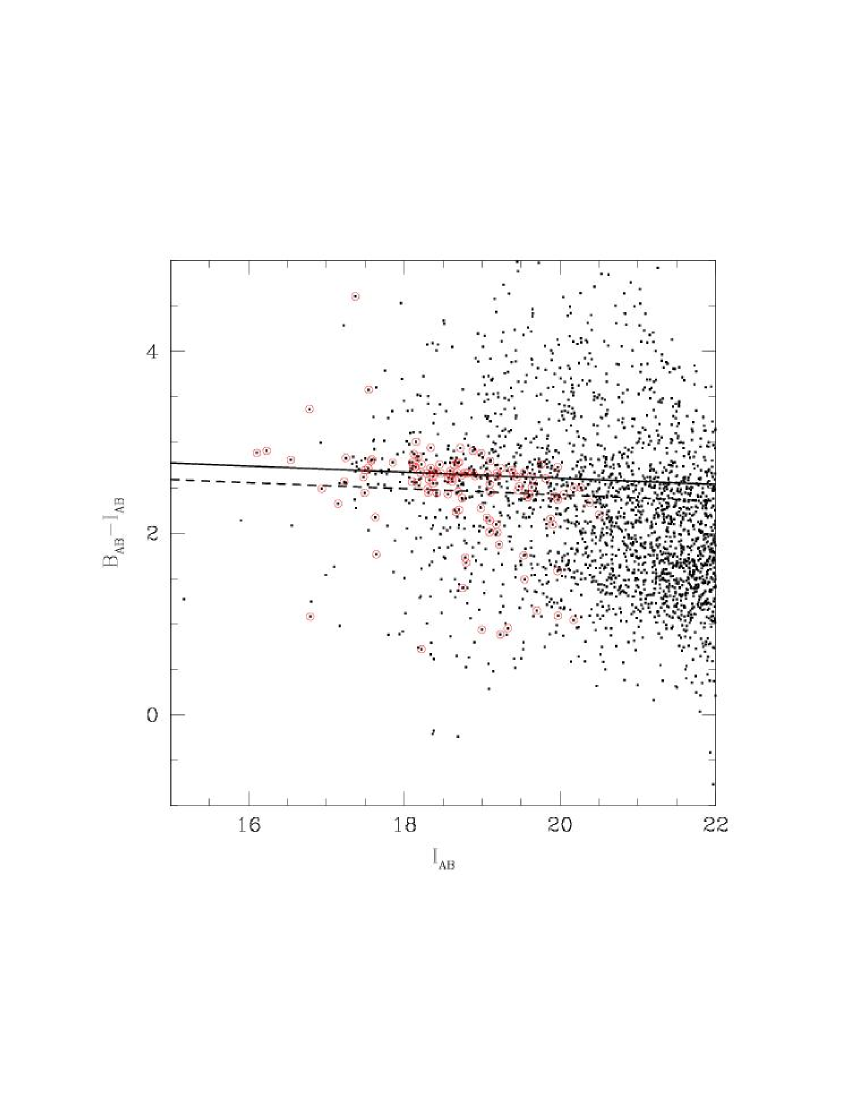
Figure 15: The color-magnitude diagram (B-I) vs. I for all the galaxies in a $15{\times}15\leavevmode\nobreak\ {\rm arcmin}^{2}$ area containing the core of the cluster. The objects represented with a circle have spectroscopic redshift and belong to the cluster. The solid straight line is the linear best-fit found for the red sequence of the elliptical galaxies of the cluster, while the dashed line represents the “boundary” between early and late type objects on the CMD.

The red sequence of the cluster has been characterized (slope, intercept and width) by considering galaxies in a smaller field ($6.8{\times}6.8\leavevmode\nobreak\ {\rm arcmin}^{2}$, ${\sim}1.5{\times}1.5\leavevmode\nobreak\ {{\rm h}_{75}}^{-2}{\rm Mpc}^{2}$) in order to reduce the higher contamination in periphery by field objects. We have used an algorithm of linear regression plus an iterated 3$\sigma$ clip, following and refining the method of Gladders et al. (1998) (detailed in Ferrari et al. in prep.). The red sequence can then be described by the linear equation ${\rm(B-I)}_{\rm AB}=-0.033{\rm I}_{\rm AB}+3.273$ with a width of 0.183 (see Fig. 15). Galaxies with measured redshift that lie within the identified red sequence and the three reddest objects of the cluster in the color-magnitude diagram have been classified as early type objects, while the galaxies with bluer colors on this diagram have been assumed to correspond to later types.

We have analyzed the galaxy velocity distribution of our sample as a function of this approximate early/late classification; histograms of velocity and distribution in projected coordinates of these objects are displayed in Fig. 16. Velocity locations and scales of the two subsamples calculated using the biweight technique are shown in Table 4.

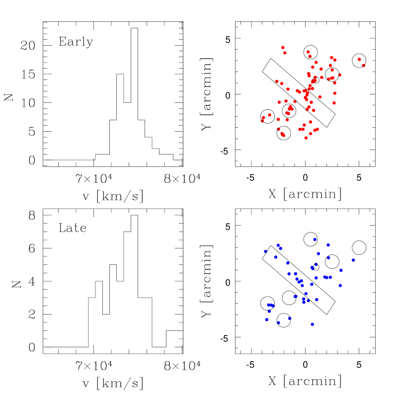
Figure 16: Top: Velocity distribution with a binning of 800 km/s (left) and projected coordinates (right) of early type galaxies. Bottom: as before, but for the late type subsample.

We find significantly different velocity dispersions for the two samples, with an extremely high value for the late type sub-sample, while quite close to the value of the main cluster component (KMM-B) for the early type one.

A trend in location is also detected, with the late type objects located at a lower velocity as compared to the early type sample. A Kolmogorov-Smirnov test rejects the hypothesis that the two velocity datasets are drawn from the same parent population with a significance level of $\sim$5.5% (see table 9). The distribution in projected coordinates is also very different for the two samples (Fig. 16, right panels). Most of the early type galaxies are aligned with the S2 axis and populate the region of the BCG and the groups, with some sparse objects in the outskirts, whereas the galaxies of the late type sample are mainly located along the S1 filament and in the external regions of the cluster, with very few objects in the South. This is confirmed by the velocity histograms plotted in Fig. 11 for each slice of Fig. 10, where the counts in velocity bins are encoded with a different color for each morphological type (blue for late, red for early). The region of the ridge (slice 2) is the richest in late type objects ($\sim 50\%$ versus $\sim 28\%$ for slices 1 and 3), in particular in the low velocity tail.

We have then investigated if this strong morphological segregation could be related at least partially to a luminosity segregation. Using the previous classification, we have converted apparent magnitudes to absolute ones, assuming k and e-corrections for E and Sa models given by Poggianti (1997). We have then divided the catalogue in three subsamples in absolute magnitudes, corresponding to ${\rm I}_{\rm AB}{\leq}{{\rm I}_{\rm AB}}^{*}$, ${{\rm I}_{\rm AB}}^{*}<{\rm I}_{\rm AB}<{{\rm I}_{\rm AB}}^{*}+2$, ${\rm I}_{\rm AB}{\geq}{{\rm I}_{\rm AB}}^{*}+2$ (with ${{\rm I}_{\rm AB}}^{*}=-22.7$, derived using the ${\rm i^{\prime}}^{*}$ value in Goto et al. 2002 and following the indication of Fukugita et al. 1995 for transforming i’ in ${\rm I}_{\rm AB}$), in order to test if the spatial and velocity distribution differs for various luminosity classes within the cluster. In table 4 we report the results for each sub-sample.

In Fig. 17, we display the projected distributions and the velocity histograms for the three tested subsamples. As a first evidence, the velocity dispersion increases drastically from brightest to faintest objects, with more than a factor two between the value obtained for the ${\rm I}_{\rm AB}{\leq}{{\rm I}_{\rm AB}}^{*}$ sample towards the ${\rm I}_{\rm AB}{\geq}{{\rm I}_{\rm AB}}^{*}+2$ one. There is also some indication of shift in location, as the brightest sub-sample is characterized by a mean velocity $\sim$700 km/s higher than the fainter ones.

Figure 17: Spatial and velocity (with a binning of 800 km/s) distribution for the three ${\rm I}_{\rm AB}$ magnitude subsamples of A521 galaxies. Top: ${\rm I}_{\rm AB}{\leq}$-22.7 - Middle: -22.7$<{\rm I}_{\rm AB}<$-20.7 - Bottom: ${\rm I}_{\rm AB}{\geq}$-20.7

The brightest galaxies lie only on the main axis of the cluster (S2), while the faintest ones are preferentially located along S1 with some galaxies in the outskirts. We have then tested for correlations between the pseudo-spectral type and luminosity class distributions. The late type subsample and the faint one have extremely similar distributions both in velocity and in projected positions; in both cases, a K-S test indicates that they are drawn from the same distribution function with high significance levels (more than 99% and 94%, Table 9). On the other side, both the velocity and the projected position distributions of the early type and of the intermediately luminous objects are drawn from the same parent population with a significance level of more than 97%, while the early type and the brightest galaxies have significance levels higher than 80%.

Table 8: Significances (%) given by the Kolmogorov-Smirnov Test for the velocity distributions of the three slices of Fig. 10

	Slice 1	Slice 2	Slice 3
Slice 1	–	37.4	27.1
Slice 2	–	–	12.3

Table 9: Significances given by the Kolmogorov-Smirnov Test for the velocity (top) and spatial (bottom) distributions of the various detected sub-samples

Significances (%)
for velocity distributions
	Early	Late	Bright	Interm.	Faint
Early	–	5.7	81.8	97.9	22.2
Late	–	–	34.8	30.7	99.7
Bright	–	–	–	58.7	20.4
Interm.	–	–	–	–	56.1
Significances (%)
for projected position distributions
	Early	Late	Bright	Interm.	Faint
Early	–	47.4	87.2	99.9	69.8
Late	–	–	77.0	92.6	94.2
Bright	–	–	–	77.0	64.3
Interm.	–	–	–	–	35.6

We have also analyzed separately the population of emission lines (15 objects) versus non emission lines galaxies (110 objects) (Fig. 18). When excluding emission lines galaxies, the location remains comparable but the velocity dispersion is notably smaller than that of the whole sample (Table 4). As shown by the histogram in Fig. 18, the velocity distribution of emission lines galaxies consists of a major concentration at low velocity (around 70000 km/s) and several isolated objects spanning the whole range of the cluster. Considering these objects together with the non-emission lines objects results in strongly enhancing the global velocity dispersion.

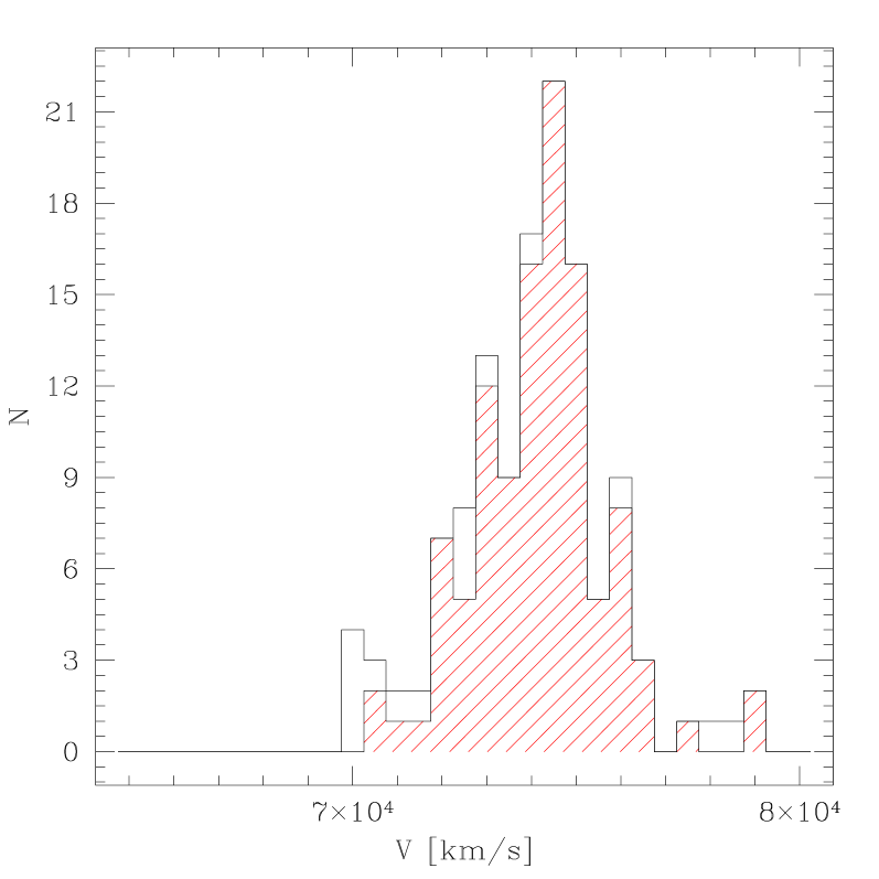
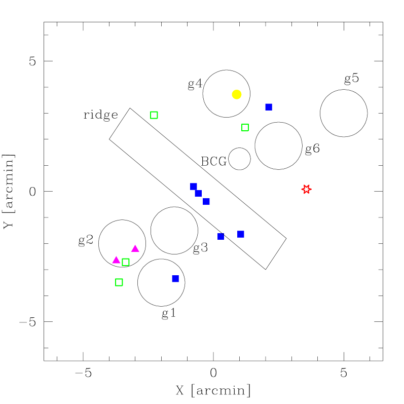
Figure 18: Left: Velocity distribution (with a binning of 500 km/s) for galaxies with (white) and without (shading) emission lines. Right: Projected coordinates of the emission line galaxies. Solid squares: ${\rm v}_{r}=69000{\div}72000$ -  Open squares: ${\rm v}_{r}=72000{\div}73000$ -  Solid circles: ${\rm v}_{r}=74000{\div}75000$ -  Stars: ${\rm v}_{r}=75000{\div}76000$ -  Triangles: ${\rm v}_{r}=76000{\div}80000$. On the electronic version of the article, colors of the symbols have the same meaning as in Fig. 10.

6 Discussion and Conclusions

The velocity distribution of Abell 521 is definitively very complex. The large value of the velocity dispersion ($\sim$ 1325 km/s) of our whole spectroscopical sample of 125 galaxies clearly results from the mixture of several components. The main features of the velocity distribution are summarized hereafter:

i) a high velocity tail in the velocity distribution is revealed by a KMM partition. From the analysis of the projected positions and of the velocity/radius diagram, these objects are found to lie in the South-East region at about 870 ${{\rm h}_{75}}^{-1}$ kpc from the X-ray main center of the cluster, and to have velocities higher than 1500 km/s as compared to the other objects at the same radius. The two-body criteria shows that the probability that this system is not bound to the main component of the cluster is quite high. These objects are probably field galaxies or a loose background group. When excluding these galaxies, the mean location remains unchanged ($\sim$ 74000 km/s), but the scale reduces slightly ($\sim$ 1200 km/s).

ii) The velocity distribution in the high density central ridge shows a velocity location systematically lower than for the whole cluster, and a very high velocity dispersion ($1780^{+234}_{-142}$ km/s). Moreover the ratio of late/early type objects are higher than in the other slices (0.95 versus 0.46 in slice 1, and 0.48 in slice 3). This region is also particularly rich in emission-line galaxies, as it contains one third of the emission line objects detected in the whole sample. The late type, emission-line objects coincide with the low velocity tail of the distribution (v$<$72000 km/s, Figs. 11 and 18). Therefore, we are witnessing a very unusual configuration in the core of the cluster: a filamentary structure of ${\sim}\leavevmode\nobreak\ 1\leavevmode\nobreak\ {{\rm h}_{75}}^{-1}$ Mpc, with galaxies showing a very broad velocity dispersion with an excess of low velocity objects, colors typically bluer than the mean, and the presence of several emission line galaxies.

iii) Various groups lie along the main NW/SE axis of the cluster. First, the region including the complex around the BCG ($\sim$ 240 ${{\rm h}_{75}}^{-1}$ kpc) appears as a strongly bound system with a very low velocity dispersion ($\sim\leavevmode\nobreak\ 250$ km/s) typical of a group and a location higher than the whole cluster($\sim\leavevmode\nobreak\ 74340$ km/s). Other groups with comparable values of location are observed: g4 at the NE extent and the southern group g3. The other groups are less well-sampled, so the following results have to be taken with caution. The northern group g6 shows a slightly lower location, while at South, g1 seems to belong to a higher velocity complex, and g2 result of superposition effects.

From these results, we can refine the scenario of formation of the cluster. The northern region is characterized by a lower velocity dispersion and a slightly higher location; it hosts a group dynamically bound to the BCG; it is clearly associated to the compact group in X-ray, which is probably falling on the main cluster (Arnaud et al. 2000). The small difference in the mean velocity of the northern region as compared to the whole cluster ($\sim\leavevmode\nobreak\ 250$ km/s in the rest-frame of the cluster) suggests that the merging occurs partly in the plane of the sky, along the North-West/South East direction S2. This direction emerges as the main axis of the ongoing merging event. Most of the detected clumps are aligned along this direction. Moreover, the early type objects as well as the brightest ones (L$>{\rm L}^{*}$) follow the general NW/SE skeleton of the cluster.

However, our scenario has also to reproduce the peculiar features that appear in the central region of the cluster, in particular its high velocity dispersion, its lower location, and its filamentary NE/SW structure. The high velocity dispersion is mostly due to the presence of the low velocity component detected by both the KMM partition and the velocity profiles. It could consist of a foreground group currently interacting with the main cluster. It is separated in radial velocity space by $\sim\leavevmode\nobreak\ 3000$ km/s from the main cluster component. This high velocity bulk flow could result from a recent merger with a significant component along the line of sight direction. Such high-speed encounters can be detected in merging clusters, as shown for instance in the case of Cl0024+1654 (Czoske et al. 2002). The high density ridge S1 would then be the projection of the merging axis along the plane of the sky. The large fraction of late type and star-forming objects along S1, coincident with the objects of the low velocity partition KMM-A, corroborates this hypothesis. In fact, a strong compression of the gas perpendicularly to the axis of the merger between the two components is expected during the merging event, which could trigger star formation in this region (Caldwell et al. 1993, Caldwell & Rose 1997, Bekki 1999). Moreover, the brightest galaxy in the eastern side of the ridge shows the same orientation as S1, and a velocity of $\sim$ 72000 km/s. This object could in fact be the original brightest galaxy of the group which has collided the main cluster.

These results imply that Abell 521 is the outcome of multiple merger processes at various stages. A denser sampling in velocity of the various groups, combined with a wider angular coverage are planned in order to understand the large-scale dynamics of this particular cluster.

Table 10: Velocity data

#	RUN	R.A.	DEC.	HEL.VEL.	ERROR	Quality flag	Emission lines
		(2000)	(2000)	v(km/s)	$\Delta$v(km/s)
1	ESO2	04:53:47.91	-10:11:23.52	89027	89	3	NO
2	ESO2	04:53:48.34	-10:11:49.60	73101	39	1	NO
3	ESO1	04:53:49.70	-10:13:32.42	33000	187	3	NO
4	ESO2	04:53:49.94	-10:11:18.81	75683	51	1	NO
5	ESO1	04:53:50.26	-10:12:19.00	25724	109	1	H$\alpha$,H$\beta$,OIII
6	ESO2	04:53:50.96	-10:10:17.04	74317	100	3	NO
7	ESO1	04:53:51.55	-10:12:42.90	-2	-2	1	NO
8	ESO2	04:53:52.01	-10:11:52.27	-2	-2	1	NO
9	ESO1	04:53:52.05	-10:12:31.30	74010	95	1	NO
10	ESO1	04:53:52.63	-10:13:23.50	-2	-2	1	NO
11	ESO2	04:53:53.19	-10:10:44.00	-1	-1	4	NO
12	ESO1	04:53:53.86	-10:12:23.32	71668	124	2	NO
13	ESO2	04:53:54.46	-10:12:29.41	-2	-2	1	NO
14	ESO1	04:53:54.75	-10:12:19.65	74144	66	1	NO
15	ESO2	04:53:54.81	-10:10:51.80	-2	-2	1	NO
16	ESO1	04:53:55.45	-10:15:01.01	74017	73	1	NO
17	ESO2	04:53:56.40	-10:10:02.15	74784	57	1	NO
18	ESO1	04:53:56.44	-10:13:26.80	76181	139	1	NO
19	ESO1	04:53:56.56	-10:14:46.29	75202	122	1	NO
20	ESO2	04:53:56.66	-10:11:41.18	-1	-1	4	NO
21	ESO1	04:53:57.33	-10:14:09.88	67749	86	2	NO
22	ESO1	04:53:57.82	-10:14:24.45	-1	-1	4	NO
23	ESO2	04:53:58.10	-10:12:09.25	74772	63	1	NO
24	ESO1	04:53:58.60	-10:14:20.41	74584	80	1	NO
25	ESO1	04:53:58.77	-10:13:25.85	71170	71	1	NO
26	ESO2	04:53:58.95	-10:11:26.08	72694	38	1	NO
27	ESO2	04:53:59.29	-10:13:01.14	121075	78	2	NO
28	ESO1	04:53:59.39	-10:13:13.00	-2	-2	1	NO
29	ESO2	04:53:59.51	-10:12:59.92	73455	34	1	NO
30	ESO1	04:53:59.93	-10:13:01.63	73033	52	1	NO
31	ESO2	04:54:00.17	-10:11:14.58	74250	40	1	NO
32	ESO1	04:54:00.27	-10:14:05.13	74574	112	1	NO
33	ESO2	04:54:00.54	-10:11:55.59	76219	49	1	NO
34	ESO1	04:54:00.70	-10:13:09.70	182923	129	1	OII
35	ESO2	04:54:01.17	-10:12:23.14	74657	114	1	NO
36	ESO2	04:54:01.41	-10:11:16.30	71490	100	1	OII,OIIIa,b,H$\beta$
37	ESO1	04:54:01.62	-10:14:07.20	73928	67	1	NO
38	ESO1	04:54:01.75	-10:12:34.47	99494	90	1	OII,H$\beta$
39	ESO2	04:54:02.16	-10:11:09.73	193062	100	3	NO
40	ESO2	04:54:02.26	-10:12:49.86	99810	100	1	OII,Balmer,H$\beta$
41	ESO1	04:54:02.34	-10:14:04.40	70301	101	1	NO
42	ESO1	04:54:02.61	-10:13:01.78	73195	92	2	OII
43	ESO2	04:54:02.97	-10:11:29.06	-2	-2	1	NO
44	ESO1	04:54:03.26	-10:13:22.40	39765	88	1	NO
45	ESO2	04:54:03.91	-10:12:15.68	74900	111	1	NO
46	ESO1	04:54:04.02	-10:14:42.44	73981	98	1	NO
47	ESO2	04:54:04.02	-10:09:22.45	-2	-2	1	NO
48	ESO1	04:54:04.12	-10:14:21.10	-2	-2	1	NO
49	ESO2	04:54:04.48	-10:11:54.81	-2	-2	1	NO
50	ESO1	04:54:04.58	-10:14:14.43	218349	70	2	NO

#	RUN	R.A.	DEC.	HEL.VEL.	ERROR	Quality flag	Emission lines
		(2000)	(2000)	v(km/s)	$\Delta$v(km/s)
51	ESO2	04:54:04.63	-10:17:31.71	72713	62	1	NO
52	ESO1	04:54:04.90	-10:12:03.68	72802	82	1	OII,H$\beta$,OIIIa,b
53	ESO1	04:54:05.06	-10:16:04.27	69854	89	1	H$\beta$,OIIIa,b
54	ESO2	04:54:05.24	-10:10:31.13	1	0	1	QSO
55	ESO1	04:54:05.48	-10:14:10.80	74959	112	1	NO
56	ESO2	04:54:05.55	-10:17:37.33	74862	71	1	NO
57	ESO1	04:54:05.60	-10:11:15.50	-2	-2	1	NO
58	ESO2	04:54:05.79	-10:11:41.71	74225	77	1	NO
59	ESO1	04:54:05.98	-10:13:16.60	74571	50	1	NO
60	ESO2	04:54:06.20	-10:12:39.05	-2	-2	1	NO
61	ESO2	04:54:06.36	-10:10:49.94	74214	83	1	OII,OIIIb
62	ESO2	04:54:06.36	-10:18:14.36	76171	59	1	NO
63	ESO1	04:54:06.37	-10:15:59.98	109406	194	1	OII,H$\beta$
64	ESO1	04:54:06.43	-10:13:24.76	74340	100	2	NO
65	ESO1	04:54:06.56	-10:13:21.32	74341	80	2	NO
66	ESO1	04:54:06.64	-10:15:36.00	72394	66	2	NO
67	ESO2	04:54:06.65	-10:11:06.49	-1	-1	4	NO
68	ESO1	04:54:06.94	-10:11:46.43	-2	-2	1	NO
69	ESO1	04:54:07.02	-10:16:04.20	44219	121	2	NO
70	ESO1	04:54:07.03	-10:12:07.51	74475	79	1	NO
71	ESO1	04:54:07.06	-10:17:55.90	74343	107	1	NO
72	ESO2	04:54:07.10	-10:13:16.76	74205	106	1	NO
73	ESO1	04:54:07.12	-10:12:41.25	110097	121	1	OII,H$\beta$,OIIIa,b
74	ESO1	04:54:07.14	-10:15:11.36	74110	77	1	NO
75	ESO2	04:54:07.97	-10:17:41.83	-1	-1	4	NO
76	ESO1	04:54:08.05	-10:14:01.90	74334	70	1	NO
77	ESO2	04:54:08.11	-10:10:20.47	74329	43	1	NO
78	ESO2	04:54:08.14	-10:11:11.79	74536	79	1	NO
79	ESO1	04:54:08.23	-10:14:58.59	68502	69	3	NO
80	ESO2	04:54:08.28	-10:14:32.30	74369	100	2	NO
81	ESO1	04:54:08.31	-10:17:13.59	55952	37	2	H$\beta$
82	ESO1	04:54:08.41	-10:12:41.95	75867	77	1	NO
83	ESO1	04:54:08.56	-10:15:13.65	102858	116	3	NO
84	ESO1	04:54:08.60	-10:15:50.10	75243	62	1	NO
85	ESO2	04:54:08.71	-10:18:19.19	71848	42	1	NO
86	ESO2	04:54:08.83	-10:10:48.42	74259	48	1	NO
87	ESO1	04:54:08.88	-10:14:58.00	73236	64	1	NO
88	ESO2	04:54:08.99	-10:11:06.96	109914	100	1	OII
89	ESO1	04:54:09.08	-10:15:34.90	74438	81	1	NO
90	ESO1	04:54:09.33	-10:15:10.08	40747	66	3	NO
91	ESO2	04:54:09.37	-10:14:10.47	76738	85	1	NO
92	ESO1	04:54:09.47	-10:17:11.80	75526	51	1	NO
93	ESO2	04:54:09.50	-10:16:44.87	76202	114	2	NO
94	ESO1	04:54:09.86	-10:16:03.13	72919	102	1	NO
95	ESO1	04:54:09.90	-10:14:13.40	72972	47	1	NO
96	ESO1	04:54:09.90	-10:17:34.20	78810	89	1	NO
97	ESO1	04:54:10.15	-10:12:55.40	-2	-2	1	NO
98	ESO1	04:54:10.39	-10:14:46.00	87413	90	1	NO
99	ESO1	04:54:10.58	-10:15:10.54	106523	114	1	OIIIa,b,H$\alpha$
100	ESO2	04:54:10.72	-10:11:50.05	-1	-1	4	NO

#	RUN	R.A.	DEC.	HEL.VEL.	ERROR	Quality flag	Emission lines
		(2000)	(2000)	v(km/s)	$\Delta$v(km/s)
101	ESO2	04:54:11.06	-10:17:35.16	75862	50	1	NO
102	ESO1	04:54:11.07	-10:15:32.80	-2	-2	1	NO
103	ESO2	04:54:11.54	-10:18:12.23	-2	-2	1	NO
104	ESO1	04:54:11.57	-10:15:13.02	35443	50	2	NO
105	ESO2	04:54:11.72	-10:14:35.28	70952	100	1	OII,OIIIa,b,H$\beta$
106	ESO2	04:54:12.02	-10:10:27.20	-2	-2	1	NO
107	ESO1	04:54:12.02	-10:17:59.30	-2	-2	1	NO
108	ESO2	04:54:12.31	-10:16:33.51	-2	-2	1	NO
109	ESO2	04:54:12.39	-10:14:13.68	72076	60	1	NO
110	ESO2	04:54:12.50	-10:14:20.31	70102	15	1	OII,OIIIa,b,H$\beta$
111	ESO1	04:54:12.73	-10:15:51.20	73965	36	1	NO
112	ESO1	04:54:13.02	-10:15:51.80	72985	143	1	NO
113	ESO1	04:54:13.09	-10:13:52.61	72067	100	1	NO
114	ESO2	04:54:13.10	-10:14:17.53	36789	100	3	NO
115	ESO1	04:54:13.14	-10:13:21.39	28080	59	1	NO
116	ESO1	04:54:13.19	-10:16:08.94	93150	120	2	NO
117	ESO1	04:54:13.37	-10:13:58.40	94388	113	2	NO
118	ESO1	04:54:13.39	-10:15:17.74	-1	-1	4	NO
119	ESO2	04:54:13.44	-10:11:17.66	-2	-2	1	NO
120	ESO2	04:54:13.54	-10:17:27.27	131100	100	2	OII
121	ESO2	04:54:13.90	-10:13:32.32	88714	100	1	OII,Balmer
122	ESO2	04:54:13.97	-10:11:13.55	124290	100	3	NO
123	ESO1	04:54:13.97	-10:18:02.64	76000	99	2	NO
124	ESO2	04:54:14.10	-10:14:07.49	106911	89	2	NO
125	ESO1	04:54:14.21	-10:13:43.40	107079	98	1	NO
126	ESO1	04:54:14.26	-10:13:54.26	88284	94	2	NO
127	ESO2	04:54:14.53	-10:14:43.21	89310	100	2	OII,H$\beta$,OIIIb
128	ESO1	04:54:14.55	-10:12:35.33	73619	144	2	NO
129	ESO1	04:54:14.69	-10:18:23.59	57498	70	3	NO
130	ESO2	04:54:14.77	-10:17:47.29	70191	100	1	OII,OIIIa,b,H$\beta$
131	ESO2	04:54:14.99	-10:11:21.55	86628	54	1	OII
132	ESO1	04:54:15.03	-10:13:48.87	127760	131	1	NO
133	ESO1	04:54:15.48	-10:13:54.17	75229	90	1	NO
134	ESO2	04:54:15.62	-10:17:20.94	130800	100	1	OII,Balmer
135	ESO2	04:54:15.68	-10:10:09.49	109765	40	1	NO
136	ESO1	04:54:15.76	-10:14:01.20	49153	124	2	NO
137	ESO1	04:54:15.81	-10:16:47.36	71874	101	1	NO
138	ESO1	04:54:15.88	-10:15:05.79	78411	55	2	NO
139	ESO1	04:54:16.01	-10:16:11.60	74932	92	1	NO
140	ESO1	04:54:16.05	-10:12:57.66	72704	93	1	NO
141	ESO2	04:54:16.08	-10:10:08.86	73830	122	1	NO
142	ESO2	04:54:16.13	-10:12:08.33	-2	-2	1	NO
143	ESO1	04:54:16.34	-10:16:04.61	74282	61	1	NO
144	ESO1	04:54:16.44	-10:15:09.60	73398	110	1	NO
145	ESO2	04:54:16.52	-10:17:54.33	107203	84	2	NO
146	ESO1	04:54:16.60	-10:14:30.60	73428	103	2	NO
147	ESO2	04:54:16.92	-10:18:09.91	73070	31	1	NO
148	ESO1	04:54:17.12	-10:14:25.17	71017	130	2	NO
149	ESO2	04:54:17.38	-10:10:57.66	74409	76	1	NO
150	ESO2	04:54:17.54	-10:13:05.01	98004	108	2	NO

#	RUN	R.A.	DEC.	HEL.VEL.	ERROR	Quality flag	Emission lines
		(2000)	(2000)	v(km/s)	$\Delta$v(km/s)
151	ESO1	04:54:17.57	-10:18:00.56	75611	88	1	NO
152	ESO1	04:54:17.93	-10:18:04.53	-2	-2	1	NO
153	ESO2	04:54:18.17	-10:10:30.22	74556	67	1	NO
154	ESO2	04:54:18.19	-10:13:38.63	72587	75	1	NO
155	ESO1	04:54:18.39	-10:13:22.62	31052	113	3	NO
156	ESO2	04:54:18.43	-10:16:50.73	88515	91	1	OII
157	ESO2	04:54:18.56	-10:13:39.25	97693	43	1	OII,H$\beta$,OIIIa,b
158	ESO1	04:54:18.87	-10:18:12.17	74546	75	1	NO
159	ESO2	04:54:18.87	-10:11:42.93	72600	121	1	OII
160	ESO2	04:54:18.92	-10:15:16.89	74785	62	1	NO
161	ESO2	04:54:19.08	-10:16:35.20	63328	96	2	NO
162	ESO1	04:54:19.23	-10:15:19.14	92338	88	2	NO
163	ESO1	04:54:19.32	-10:16:45.17	109151	74	1	OII
164	ESO1	04:54:19.75	-10:13:49.60	-2	-2	1	NO
165	ESO2	04:54:19.78	-10:11:27.08	75907	87	1	NO
166	ESO2	04:54:20.06	-10:13:28.71	73571	91	1	NO
167	ESO1	04:54:20.53	-10:10:22.20	-2	-2	1	NO
168	ESO1	04:54:20.65	-10:17:26.06	99128	89	2	NO
169	ESO2	04:54:20.92	-10:13:55.87	-2	-2	1	NO
170	ESO1	04:54:20.96	-10:16:44.77	78326	146	1	OII,H$\beta$
171	ESO2	04:54:21.12	-10:09:39.91	-2	-2	1	NO
172	ESO1	04:54:21.29	-10:12:07.41	101738	64	2	NO
173	ESO1	04:54:21.30	-10:14:46.26	55236	86	2	NO
174	ESO2	04:54:21.63	-10:12:02.65	-1	-1	4	NO
175	ESO1	04:54:21.65	-10:16:41.02	73571	64	1	NO
176	ESO1	04:54:22.20	-10:14:50.23	-2	-2	1	NO
177	ESO2	04:54:22.32	-10:16:25.27	73694	51	1	NO
178	ESO1	04:54:22.35	-10:17:13.40	72593	107	1	H$\beta$
179	ESO1	04:54:22.64	-10:16:40.67	79233	125	1	NO
180	ESO2	04:54:22.70	-10:15:13.01	54106	71	1	H$\beta$,OIIIa,b
181	ESO2	04:54:23.18	-10:17:58.06	72568	93	1	OII,OIIIa,b,H$\beta$
182	ESO1	04:54:23.19	-10:12:38.32	-2	-2	1	NO
183	ESO2	04:54:23.25	-10:11:33.53	88370	59	1	NO
184	ESO1	04:54:23.73	-10:13:05.92	109876	144	2	NO
185	ESO1	04:54:23.73	-10:17:10.67	78122	100	1	H$\beta$
186	ESO2	04:54:23.93	-10:11:26.49	88524	50	1	NO
187	ESO1	04:54:24.16	-10:14:00.74	-2	-2	3	NO
188	ESO1	04:54:24.55	-10:16:40.88	73983	48	1	NO
189	ESO1	04:54:24.60	-10:14:12.10	106221	88	1	OII,H$\beta$,OIIIa,b
190	ESO1	04:54:24.77	-10:14:14.81	75310	84	3	NO
191	ESO1	04:54:24.91	-10:16:58.01	72929	69	1	NO

References

- (1) Arnaud, M., Maurogordato, S., Slezak, E., & Rho, J., 2000, A&A, 355, 461
- (2) Ashman, K.M., Bird, C.M., & Zepf, S., 1994, AJ, 108, 2348
- (3) Bardelli, S., Pisani, A., Ramella, M., Zucca, E., & Zamorani, G., 1998, MNRAS, 300, 589
- (4) Beers, T. C., Gebhardt, K., Forman, W., Huchra, J. P., & Jones, C., 1991, AJ, 102, 1581
- (5) Beers, T. C., Flynn, K., & Gebhardt, K., 1990, AJ, 100, 32
- (6) Beers, T. C., Geller, M. J., & Huchra, J. P., 1982, ApJ, 257, 23
- (7) Bekki, K., 1999, ApJ, 510, L15
- (8) Berrington, R.C., Lugger, P.& M., Cohn, H. N., 2002, AJ, 123, 2261
- (9) Bird, C. M., 1994, AJ, 107, 1637
- (10) Bird, C. M., & Beers, T. C., 1993, AJ, 105, 1596
- (11) Caldwell, N., & Rose, J., 1997, AJ, 113, 492
- (12) Caldwell, N., Rose, J., Sharples, R., Ellis, R., & Bower, R., 1993, AJ, 106, 473
- (13) Czoske, O., Moore, B., Kneib, J.-P., & Soucail, G., 2002, A&A, 386, 31
- (14) Donnelly, R. H., Forman, W., Jones, C., Quintana, H., Ramirez, A., Churazov, E., & Gilfanov, M., 2001, ApJ, 562, 254
- (15) Dressler A., & Shectman, S., 1988, AJ, 95, 985
- (16) Dressler A., 1980, ApJ, 236, 351
- (17) Ellis, R. S., Smail, I., Dressler, A., Couch, W. J., Oemler, A., Jr., Butcher, H., & Sharples, R. M., 1997, ApJ, 483, 582
- (18) Flores, R. A., Quintana, H., & Way, M. J., 2000, ApJ, 532, 206
- (19) Fukugita, M., Shimasaku, K., & Ichikawa, T., 1995, PASP, 107, 945
- (20) Geller, M. J., & Beers, T. C., 1982, PASP, 94, 421
- (21) Girardi, M., Escalera, E., Fadda, D., Giuricin, G., Mardirossian, F., & Mezzetti, M., 1997, ApJ, 482, 41
- (22) Gladders, M. D., Lopez-Cruz, O., Yee, H. K. C., & Kodama, T., 1998, ApJ, 501, 571
- (23) Goto, T., Okamura, S., & Brinkmann, J., to be published in PASJ vol.54 No.4, August 25, 2002
- (24) Hanisch, R. J., & Ulmer, M. P., 1985, AJ, 90, 1407
- (25) Hartigan, J. A., & Hartigan, P. M., 1985, The Annals of Statistics, Vol.13, No. 1, 70-84
- (26) Johnson, M. W., Cruddace, R. G., Wood, K. S., Ulmer, M. P., & Kowalski, M. P., 1983, ApJ, 266, 425
- (27) Jones, C., & Forman, W., 1992, in Clusters and Superclusters of Galaxies, ed. A. C. Fabian (Dodrecht: Kluwer), 49
- (28) Kauffmann G., & White, S. D. M., 1993, MNRAS, 261, 921
- (29) Kodama, T., Bower, R. G., & Bell, E. F., 1999, MNRAS, 306, 561
- (30) Kowalski, M. P., Cruddace, R. G., Wood, K. S., & Ulmer, M. P., 1984, ApJS, 56, 403
- (31) Lacey, C. G., & Cole, S., 1993, MNRAS, 262, 627
- (32) McLachlan, G. J., Basford, K. E., 1988, Mixture Models (Marcel Dekker, New York)
- (33) Maurogordato, S., Proust, D., Beers, T. C., Arnaud, M., Pellò, R., Cappi, A., Slezak, E., & Kriessler, J. R., 2000, A&A, 355, 848
- (34) Maurogordato S., Le Fevre O., Proust D., Vanderriest C., & Cappi A., 1996, BCFHT 34, 5
- (35) Mohr, J. J., Geller, M. J., Fabricant, D. G., Wegner, G., Thorstensen, J., Richstone, D. O., 1996, ApJ, 470, 724
- (36) Mohr, J. J., Evrard, A. E., Fabricant, D. G., & Geller, M. J., 1995, ApJ, 447, 8
- (37) Poggianti, B.M., 1997, A&AS, 122, 399
- (38) Richstone, D., Loeb, A., Turner, & E. L., 1992, ApJ, 393, 477
- (39) Rose, J. A., Gaba, A. E., & Christiansen, W. A., 2002, AJ, 123, 1216
- (40) Serna, A., & Gerbal, D., 1996, A&A, 309, 65
- (41) Tonry, J., & Davis, M., 1981, ApJ, 246, 666
- (42) Ulmer, M. P., Cruddace, R. G., &, Kowalski, M. P., 1985, ApJ, 290, 551
- (43) Valtchanov, I., Murphy, T., Pierre, M., Hunstead, R., &, Lémonon, L., astro-ph/0206415
- (44) West, M. J., & Bothun, G. D., 1990, ApJ, 350, 36