ON THE CONNECTION BETWEEN MEAN FIELD DYNAMO THEORY AND FLUX TUBES

Abstract

Mean field dynamo theory deals with various mean quantities and does not directly throw any light on the question of existence of flux tubes. We can, however, draw important conclusions about flux tubes in the interior of the Sun by combining additional arguments with the insights gained from solar dynamo solutions. The polar magnetic field of the Sun is of order 10 G, whereas the toroidal magnetic field at the bottom of the convection zone has been estimated to be 100,000 G. Simple order-of-magnitude estimates show that the shear in the tachocline is not sufficient to stretch a 10 G mean radial field into a 100,000 G mean toroidal field. We argue that the polar field of the Sun must get concentrated into intermittent flux tubes before it is advected to the tachocline. We estimate the strengths and filling factors of these flux tubes. Stretching by shear in the tachocline is then expected to produce a highly intermittent magnetic configuration at the bottom of the convection zone. The meridional flow at the bottom of the convection zone should be able to carry this intermittent magnetic field equatorward, as suggested recently by Nandy and Choudhuri (2002). When a flux tube from the bottom of the convection zone rises to a region of pre-existing poloidal field at the surface, we point out that it picks up a twist in accordance with the observations of current helicities at the solar surface.

1 Introduction

Observations of the solar surface clearly indicate that the magnetic field there exists in the form of flux tubes. We see magnetic flux concentrations of various sizes, from large sunspots to fibril flux tubes at the limit of seeing. There is no direct observational evidence whether the magnetic field exists in the form of flux tubes even in the interior of the convection zone. Various theoretical considerations, however, suggest that this must be so due to the interaction of the magnetic field with the surrounding convection. Simulations of flux tube rise explain various aspects of bipolar active regions on the surface rather well, suggesting that the magnetic field probably rises as flux tubes from the bottom of the convection zone (Choudhuri, 1989; D’Silva and Choudhuri, 1993; Fan, Fisher, and DeLuca, 1993; Caligari, Moreno-Insertis, and Schüssler, 1995; Longcope and Fisher, 1996; Longcope and Choudhuri, 2002).

One of the important problems in solar physics is to understand the generation of the solar magnetic field by the dynamo process (for a recent review, see Choudhuri, 2002). Since doing a full dynamical simulation of the dynamo process in the entire solar convection zone is an extremely difficult problem (Gilman, 1983; Glatzmaier, 1985), most of the solar dynamo models are of kinematic nature and are based on the mean field dynamo equation (Moffatt, 1978, Ch. 7; Choudhuri, 1998, Ch. 16). This mean field equation is obtained by averaging over the fluctuating magnetic and velocity fields. If the magnetic field exists in the form of flux tubes, then certainly the magnetic fluctuations are much larger than the mean value. One can raise doubts whether the averaging procedure and the subsequent approximations like the first order smoothing approximation can be trusted in such a situation. The full dynamical simulations have demonstrated that the dynamo process really does take place (Gilman, 1983; Glatzmaier, 1985), even though these simulations failed to yield realistic models of the solar dynamo. We, therefore, believe that the mean field equation captures the essence of the dynamo process in some approximate way, even though it may be difficult to justify it rigorously on mathematical grounds. We shall, however, show that if one blindly follows the results of mean field theory without keeping in mind that the magnetic field exists in the form of flux tubes, then one is often drawn into misleading conclusions.

As of now, there exists no mean field formulation which addresses the issue of flux tubes. How should we then reconcile the results of mean field dynamo theory with the existence of flux tubes? The aim of this paper is to suggest the following two-step procedure:

1. First solve the mean field dynamo equation to get a qualitative idea of how the mean magnetic field behaves;

2. Then use other basic physics considerations to figure out how the magnetic field may be structured in flux tubes in different regions, leading to a more complete picture of the dynamo process.

The first step of solving the mean field equation will not be presented in this paper. We shall rather rely on the insight gained from the dynamo calculations presented in several recent papers (Choudhuri, Schüssler, and Dikpati, 1995; Durney, 1995, 1996, 1997; Dikpati and Charbonneau, 1999; Küker, Rüdiger, and Schultz, 2001; Nandy and Choudhuri, 2001, 2002). We shall explicitly carry out the second step listed above in this paper, based on the general picture of the mean magnetic field that emerges from the above dynamo calculations. In spite of some differences in the approaches of the above authors, there are many common characteristics. Since the meridional circulation plays a crucial role in the works of all the above authors, we shall refer to this type of dynamo model as the circulation-dominated solar dynamo model or CDSD model in brief.

Before carrying the second step listed above, let us summarize the general characteristics of the CDSD model on which we shall carry out our procedure. The toroidal field is produced by the stretching of poloidal field lines by differential rotation. Since helioseismology has shown that differential rotation is concentrated in the tachocline at the base of the convection zone, there is virtually universal agreement that the strong toroidal field must be produced in this tachocline. This toroidal field must rise from there to produce active regions on the solar surface. Simulations of this rise suggest that the strength of this toroidal field at the base of the convection zone must be of order 100,000 G (Choudhuri and Gilman, 1987; Choudhuri, 1989; D’Silva and Choudhuri, 1993; Fan, Fisher, and DeLuca, 1993). Since convective turbulence cannot twist such strong fields, the conventional $\alpha$-effect (Parker 1955; Steenbeck, Krause, and Rädler 1966) is unlikely to be operative. All authors working on the CDSD model have invoked the idea of Babcock (1961) and Leighton (1969) that the poloidal field is produced near the solar surface by the decay of tilted active regions. The poleward meridional circulation in the upper regions of the convection zone has been mapped to a depth of about 15% of the solar radius (Giles, Duvall, and Scherrer, 1997; Braun and Fan, 1998). To conserve mass, there has to be an equatorward return flow through the lower layers of the convection zone. The poloidal field generated at the surface is carried by this meridional circulation first poleward and then down underneath to the tachocline, where it can be stretched to produce the toroidal field. All authors working on the CDSD model agree on this general scenario and many of our deductions in this paper are based on this generally agreed scenario.

Nandy and Choudhuri (2002) have recently introduced a new idea in the CDSD model and later in this paper we shall explore some of the consequences of this idea. So we summarize this new idea here. The differential rotation $d\Omega/dr$, which has a negative value in the high latitudes within the tachocline, is much stronger there compared to what it is in the low latitudes within the tachocline, where it is positive (see Fig. 1 of Nandy and Choudhuri, 2002). A differential rotation of this kind tends to produce the strong toroidal field (and thereby enhanced magnetic activity) at high latitudes rather than at low latitudes where sunspots are seen (Durney, 1997; Dikpati and Charbonneau, 1999; Küker, Rüdiger, and Schultz, 2001; Nandy and Choudhuri, 2002). Since the meridional circulation is generally believed to be driven by the turbulent stresses of the convection zone, most authors working on the CDSD model assume the meridional circulation to be confined within the convection zone. In view of the fact that nothing much is known about the equatorward return flow of this circulation in the deeper layers of the convection zone—either from observations or from any well-established theoretical model, Nandy and Choudhuri (2002) have proposed the tentative hypothesis that this flow penetrates slightly below the convection zone, to a greater depth than usually believed. Even if the strong toroidal field is produced at high latitudes within the tachocline, this flow would take it to the stable layers below the convection zone and would not allow it to emerge at high latitudes. The toroidal field is then transported equatorward by the meridional circulation through the stable layers and comes within the convection zone only at low latitudes where the meridional flow rises. Thus, even though the toroidal field is produced in the tachocline at high latitudes, it comes within the convection zone and becomes buoyant only at low latitudes, thereby ensuring that flux eruption takes place only at the typical sunspot latitudes. We shall show that this idea has some additional attractive features when we introduce flux tube considerations with it.

We show in the next section that the shear in the tachocline is insufficient to stretch a 10 G mean polar field into a 100,000 G mean toroidal field. This fact forces us to conclude that the polar field must become intermittent before being advected to the tachocline. The geometry of the polar field before entering the tachocline is worked out in §3. Then §4 looks at the implications of an intermittent field specifically for the model of Nandy and Choudhuri (2002). Some properties of flux tubes at the bottom of the convection zone are discussed in §5. The question of magnetic helicity and twists of flux tubes is addressed in §6. Finally, some of the main points are summarized in the concluding section.

2 The stretching of field lines by differential rotation

Magnetogram observations show that the maximum radial field $B_{r}$ in the polar region can be of order 10 G. According to the CDSD model, this field is transported below by the meridional circulation sinking near the poles and then brought to the tachocline to be stretched by the differential rotation. Although the field is taken to regions of much higher density and any horizontal component will be compressed by a large factor in this process, a radial field remains more or less unaffected when it is transported by a nearly vertically downward flow. We expect that the maximum value of $B_{r}$ even at the bottom of the convection zone in the polar region to be about 10 G. This field is stretched by the differential rotation in the tachocline to generate the toroidal component. The full equation describing the evolution of the toroidal component is

$$\frac{\partial B_{\phi}}{\partial t}+\frac{1}{r}\left[\frac{\partial}{\partial r}(rv_{r}B_{\phi})+\frac{\partial}{\partial\theta}(v_{\theta}B_{\phi})\right]=\eta\left(\nabla^{2}-\frac{1}{s^{2}}\right)B_{\phi}$$ (1)

$$+s({\bf B}_{p}.\nabla)\Omega-\nabla\eta\times\left(\nabla\times B_{\phi}\bf{e_{\phi}}\right),$$

where $s=r\sin\theta$ and the other symbols have the usual meanings. It is the term $s({\bf B}_{p}.\nabla)\Omega$ which describes the generation of the toroidal field from the poloidal field due to the stretching by differential rotation. Within the tachocline, the time evolution of the toroidal field is dominated by this term. So the toroidal field generated in the tachocline is approximately given by

$$B_{\phi}\approx s({\bf B}_{p}.\nabla)\Omega\,\tau,$$

where $\tau$ is the time for which the stretching takes place. Since the differential rotation is mainly radial in the tachocline, (2) leads to

$$\frac{B_{\phi}}{B_{r}}\approx s\frac{\Delta\Omega}{\Delta r}\tau.$$

Let us now estimate the approximate value of the ratio $B_{\phi}/B_{r}$ of the toroidal field to the poloidal field from which it is produced. Since the toroidal field $B_{\phi}$ is believed to have the rather high value of 100,000 G, we use such approximate values of various quantities in (3) which would make the ratio $B_{\phi}/B_{r}$ as large as possible. Within the tachocline, $\Omega$ changes from about 2150 nHz at the top to about 2800 nHz at the bottom, so we take $\Delta\Omega\approx 650$ nHz. Let us use the rather large value $s\approx 0.5R_{\odot}$ and the rather small value $\Delta r\approx 0.1R_{\odot}$ for the thickness of the tachocline. On taking $\tau\approx 10$ yr and substituting all these values in (3), we get

$$\frac{B_{\phi}}{B_{r}}\approx 1000.$$

Thus the radial magnetic field of 10 G can be stretched to produce a toroidal field of maximum strength 10,000 G—smaller by a factor of 10 compared to the strength 100,000 G inferred from the flux tube simulations. To produce a toroidal field of 100,000 G by the stretching of the radial field, we need to begin with a radial field of order 100 G.

It is clear that a radial field of about 10 G cannot be stretched in the tachocline to produce a toroidal field of 100,000 G, as required to match surface observations in flux tube simulations. What could be amiss here? We now have to be careful not to mix up mean field arguments with flux tube arguments. The value 10 G for the radial field is the mean value appropriate for mean field theories. Although flux tube simulations tell us that the magnetic field inside a flux tube has to be 100,000 G, these simulations do not throw any light on the volume filling factor of these flux tubes at the bottom of the convection zone or on the mean value of the toroidal field there. Our equations (1)–(4) all hold for mean values. If a mean radial field of 10 G produces a mean toroidal field of 10,000 G, which is intermittently concentrated into flux tubes with field 100,000 G, then all our theoretical requirements are satisfied. This gives us a volume filling factor of about $f\approx 0.1$ for the toroidal field. Keeping in mind that our estimate of $B_{\phi}/B_{r}$ is based on values of various things which make this ratio maximum, we conclude that 0.1 is the upper limit of the filling factor $f$. The actual filling factor may be somewhat smaller than this, but probably not smaller by an order of magnitude. We thus see that we can derive an approximate value of the volume filling factor of the toroidal field from very simple considerations. An estimate of the volume filling factor would be of interest for various purposes. Within the next few years, it may be possible to use helioseismology to probe the magnetic field at the bottom of the convection zone. Apart from the theoretical expectation that the magnetic field inside flux tubes should be of order 100,000 G, an idea of the volume filling factor would give helioseismologists a good clue of what to look for.

There are two possible routes through which we may obtain toroidal flux tubes with 100,000 G field starting from a radial field of 10 G:

1. A fairly uniform $B_{r}\approx 10$ G may first give rise to a fairly uniform $B_{\phi}\approx 10,000$ G, which then gets broken into toroidal flux tubes with magnetic field 100,000 G.

2. A fairly uniform $B_{r}\approx 10$ G may first get broken into vertical flux tubes with field of order 100 G and then these vertical flux tubes may be stretched in the tachocline to produce toroidal flux tubes with field 100,000 G.

We here argue in favour of the second possibility. The magnetic field 100,000 G inside the toroidal flux tubes is much larger than the equipartition magnetic field (i.e. the magnetic field having energy density equal to the kinetic energy density of convective turbulence) at the tachocline. Convective turbulence certainly could not concentrate the magnetic field into flux tubes of such intensity. On the other hand, convective turbulence above the tachocline could easily concentrate the radial field into vertical flux tubes with field 100 G (considerably less than the equipartition value) and then these flux tubes could be stretched by the differential rotation to produce toroidal flux tubes with field 100,000 G. It is not difficult to suggest a physical scenario how the formation of the vertical flux tubes above the tachocline may come about. In a region of convection, magnetic fields tend to get concentrated in the boundaries of convection cells. This is seen at the solar surface as well as in simulations of magnetoconvection. We believe that the convection cells deeper down in the solar convection zone are bigger in size, since the scale height is larger there. So a nearly uniform radial field at the surface is pushed by the downward meridional flow into regions where convection cells are larger and consequently cell boundaries are further and further apart. The magnetic field would be pushed to these cell boundaries and would become highly intermittent. A snapshot of magnetic field lines in the vertical plane may appear as shown in Figure 1.

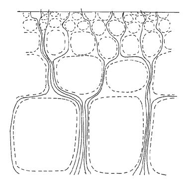
Figure 1: A sketch of magnetic field lines in a vertical plane near the polar region of the solar convection zone. The dashed lines indicate convection cells, which become larger as we go deeper.

3 Probable magnetic field geometry above and within the tachocline

We now try to figure out what the magnetic field may look like above and within the tachocline. Earlier, we had put such values of various quantities in (3) that would make the ratio $B_{\phi}/B_{r}$ as large as possible. A more reasonable value of this ratio may be

$$\frac{B_{\phi}}{B_{r}}\approx 200$$

rather than 1000 as given in (4). In that case, we have to begin with vertical flux tubes having inside fields $B_{r}\approx 500$ G which can be stretched in the tachocline to produce toroidal flux tubes with magnetic fields of 100,000 G inside. Since the mean value of $B_{r}$ is 10 G, we need to have a filling factor of only $f=0.02$ or $2\%$ if this mean field has to be concentrated into flux tubes of strength 500 G.

We can also draw some conclusions about the sizes of these flux tubes. We are arguing that these radial flux tubes above the tachocline in the polar region get stretched in the tachocline to produce the toroidal flux tubes and then parts of these flux tubes rise to produce the active region. Therefore, the magnetic flux associated with a vertical flux tube above the tachocline would be the flux which we would finally find as the flux in a typical sunspot, i.e.

$$B_{ft}\,r_{ft}^{2}=B_{ss}\,r_{ss}^{2}.$$

Here $B_{ft}$ is the magnetic field inside a vertical flux tube above the tachocline (estimated above to be 500 G) and $B_{ss}$ is the magnetic field inside a sunspot at the photospheric level (3000 G), whereas $r_{ft}$ and $r_{ss}$ are the corresponding radii. We then have

$$r_{ft}=r_{ss}\left(\frac{B_{ss}}{B_{ft}}\right)^{1/2}.$$

The typical radius of a flux tube above the tachocline thus has to be somewhat larger than the radius of a sunspot at the photospheric level. On taking the radius of a typical sunspot to be about 5000 km, (6) gives

$$r_{ft}\approx 12,000\;\mbox{km}.$$

In order to have a filling factor of about $f$, these flux tubes need to have typical horizontal separations of order

$$s\approx f^{-1/2}\,r_{ft},$$

which turns out to be

$$s\approx 85,000\;\mbox{km}$$

on using $f\approx 0.02$. This is of the same order as the vertical scale height at the bottom of the solar convection zone and one would naively expect the convection cells to have horizontal sizes of this order in that region. Our arguments thus lead us to the conclusion that the typical horizontal separations of these flux tubes must be of the same order as the horizontal sizes of the convection cells—a very sensible conclusion in view of the fact that we expect the flux tubes to be concentrated at the boundaries of convection cells. This remarkable conclusion gives us the confidence that we are approximately on the correct track.

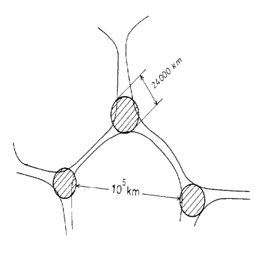
Figure 2: A sketch indicating positions of vertical magnetic flux tubes (shaded regions) in a horizontal plane some distance above the tachocline, in the polar region of the solar convection zone. The curved lines indicate boundaries of convection cells, where the fluid is sinking.

Figure 2 gives a sketch of how the vertical flux tubes would appear distributed in a horizontal section somewhat above the tachocline in the polar region. The radii of the flux tubes are of order 12,000 km and their separations are of order 85,000 km. If the magnetic field inside flux tubes is of order 500 G, then the mean magnetic is clearly of order 10 G. The separations between the flux tubes being quite large, at any time there would be only a few vertical flux tubes in the polar region above the tachocline. However, these few flux tubes are expected to be quite long-lived, since the convective turnover time in this region is of the order of months. These flux tubes are expected to be advected downward inside the tachocline, where they get stretched in the toroidal direction by the differential rotation. What would the resulting distribution of toroidal flux tubes look like? Since the vertical flux tubes above the tachocline had finite lengths (as seen in Figure 1), we expect them to produce horizontal flux tubes of finite length, with the magnetic field somewhat diffuse amongst these concentrated flux tubes of finite length. Figure 3 shows how the magnetic flux in the tachocline may be distributed as seen from above.

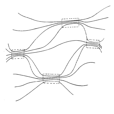
Figure 3: A sketch showing magnetic field lines at the bottom of the solar convection zone, as seen from above.

4 Equatorward advection of magnetic flux, magnetic buoyancy and formation of active regions

We know that magnetic buoyancy is particularly destabilizing inside the convection zone, but can be suppressed to a large extent in the sub-adiabatic region below the bottom of the convection zone (see, for example, Parker, 1979, §8.8). The usual scenario of active region formation is the following. The toroidal flux tubes remain stored in the stable layers below the bottom of the convection zone. Occasionally a part of a toroidal flux tube may be pushed into the convection zone, perhaps due to the disturbances caused by overshooting plumes getting into the stable layers. Once a part of a flux tube has entered the convection zone, it becomes buoyant and rises in the form of a loop, eventually to produce bipolar active regions (Moreno-Insertis, 1986; Choudhuri, 1989). In this view, only a small portion of a flux tube makes it to the solar surface. The major part of the flux tube remains anchored inside the tachocline. An active region can thus be viewed to be like the tip of an iceberg, the much larger chunk of the flux tube remaining embedded in the tachocline.

If the recent model of Nandy and Choudhuri (2002) is correct, then we are led to a radically different perspective. According to their model, the toroidal flux tubes are pushed into stable layers below the bottom of the convection zone immediately after their creation within the tachocline at high latitudes. However, when the penetrating meridional circulation rises at the low latitudes and enters the convection zone, it would carry all the flux tubes embedded in the fluid and bring everything to the convection zone. Thus the scenario of a flux tube sitting within the tachocline and only a small part of it rising could not possibly be correct if there is a meridional flow which penetrates below the tachocline and then sweeps through it at the low latitudes when it rises upward to enter the convection zone.

If the toroidal flux created within the tachocline is completely brought into the convection zone at low latitudes, then how can we explain the formation of active regions which seem to have roots anchored deep down? We get a clue by noting that magnetic field inside the tachocline is distributed as shown in Figure 3 and remembering that magnetic buoyancy is a function of magnetic field strength. Concentrated portions of a flux tube rise much more quickly than other portions. The acceleration due to magnetic buoyancy goes as $B^{2}$, whereas the terminal velocity of rise (by the braking action of drag) goes as $B$ (see, for example, Parker, 1979, §8.7). When the magnetic configuration shown in Figure 3 is brought into the convection zone by the meridional flow, the concentrated portions of magnetic flux will rise rapidly in the form of loops, whereas other diffuse portions will rise very slowly. In this view, the active regions appear anchored—not because other portions of the flux tube down at the bottom of the convection zone remain anchored, but rather because the flux tube ceases to exist as we follow magnetic field lines from the active region to the bottom of the convection zone and the diffuse magnetic field there rises much more slowly (mainly due to the advection by the upward moving meridional flow rather than magnetic buoyancy). We can make a rough estimate of the diffuse field by assuming it to be of the same order as mean $B_{\phi}$. Now, (5) should hold either for magnetic fields in local regions or for mean magnetic fields, so we write

$$\overline{B}_{\phi}\approx 200\,\overline{B}_{r}.$$

On taking $\overline{B}_{r}$ to be 10 G,

$$\overline{B}_{\phi}\approx 2000\;\mbox{G}.$$

If the diffuse field is of order 2000 G, then its rise time is of the order of several years (Parker, 1975; Moreno-Insertis, 1983), whereas the rise time of the concentrated portion with field 100,000 G is of the order of a few weeks. The rise of the concentrated portions of magnetic field would be exactly like the rise of the upper parts of flux loops in the earlier scenario of flux tubes going into the stable layers where anchoring took place, and we believe that most of the important results of numerical simulations based on the earlier scenario (Choudhuri, 1989; D’Silva and Choudhuri, 1993; Fan, Fisher, and DeLuca, 1993; D’Silva and Howard 1993; Caligari, Moreno-Insertis, and Schüssler, 1995) should carry over to the new scenario.

Although this new scenario may appear radical at the first sight, we are not aware of any arguments against it. The new scenario retains all the attractive aspects of the old scenario. Additionally, the new scenario solves some problems which would find no easy solution in the old scenario. We now turn to these problems.

4.1 The diffusion problem

The magnetic field of the Sun reverses its direction every 11 years. If the active regions are merely tips of icebergs and major portions of flux tubes are stored at the bottom of the convection zone, then these stored flux tubes have to be destroyed in less than 11 years. It is not clear how this could have happened. Certainly the resistivity of the plasma is too small to achieve this. The only possibility left is turbulent diffusion. If the magnetic field is as strong as 100,000 G, then even turbulence will not be able to distort these flux tubes and mix them up (Parker, 1993). In kinematic models of the solar dynamo, one usually chooses some value of turbulent diffusion which makes various things come out right. But there is no physical basis for assuming such turbulent diffusion if the magnetic field is of order 100,000 G. It has, therefore, remained a complete mystery in the solar dynamo problem how the flux tubes with very strong magnetic field at the bottom of the convection zone get destroyed in a few years.

In the new scenario we are proposing, this problem is solved in one single stroke. We are suggesting that magnetic fields seen on the surface do not constitute the tip of an iceberg, but they are all there is to it. There is no further magnetic flux sitting at the bottom of the convection zone and waiting to disappear in a few years by some mysterious process. The concentrated parts of the magnetic field float to the surface due to magnetic buoyancy, whereas the diffuse parts which rise slowly can be mixed up by turbulence and destroyed. According to the Babcock-Leighton idea, the poloidal field at the surface is produced from the decay of active regions (Babcock, 1961; Leighton, 1969), and we know that the poloidal field is then freely advected poleward by the meridional circulation (Wang, Nash, and Sheeley, 1989; Dikpati and Choudhuri, 1994, 1995). If the active regions remained anchored to flux tubes underneath the bottom of the convection zone, then it would have been difficult for the poloidal field to be detached so easily and then to be carried poleward. In the scenario we are suggesting, it should be possible for the poloidal field to be detached more easily. Recent work by Longcope and Choudhuri (2002) suggests that active regions do not get disconnected at a shallow depth soon after the formation. Presumably they eventually get disconnected when the diffuse portions beyond the ends of the flux tubes deep down in the convection zone get mixed up by turbulence.

4.2 The magnetic tension problem

In the model of Nandy and Choudhuri (2002), the toroidal flux tubes are carried by the meridional flow from high latitudes to low latitudes through the stable layers just below the bottom of the convection zone. If the flux exists in the form of a toroidal flux ring symmetric around the rotation axis, then we know that it has to stretched if we want to take it from a high latitude to a low latitude and such stretching involves working against magnetic tension. For a magnetic field of strength 100,000 G the magnetic tension would be very large, even though the magnetic pressure would still be only about $10^{-5}$ of the gas pressure and only a small perturbation in the gas pressure will be needed to overcome the magnetic forces. However, the kinetic energy density associated with the meridional flow would be much less than the energy density of a 100,000 G magnetic field. So, one possible objection against the model of Nandy and Choudhuri (2002) is that the meridional flow will not be able to carry the magnetic flux to low latitudes by working against the large magnetic tension (Gilman, private communication).

This objection disappears in the scenario we are now proposing. We are suggesting that strong magnetic tubes are highly intermittent and are of finite length beyond which the magnetic field becomes diffuse, i.e. there are no flux rings going all the way round the rotation axis. The magnetic tension goes as $B^{2}$ and the tension of the diffuse field is much less. According to (10), the diffuse field is of order 2000 G and the energy density associated with it is about $10^{5}$ c.g.s. Equating this to $\rho v^{2}/2$ and taking $\rho=0.2$ gm cm^-3, we get

$$v\approx 10\;\mbox{m s}^{-1}.$$

In other words, a meridional flow having a velocity larger than 10 m s^-1 at the bottom of the convection zone would have more energy density than the diffuse magnetic field and would be able to carry it. The poleward flow velocity at the surface is of order 20 m s^-1. Although we have no direct knowledge of the value of equatorward meridional flow at the bottom of the convection zone, it is expected to be a few m s^-1 and most kinematic dynamo calculations assume such values to get the best results. Such a meridional flow may just have the right strength to carry the diffuse magnetic field, without its tension being able to pose a serious problem. It would be difficult for the meridional flow to stretch the bundles of concentrated field any further. But the concentrated bundles of flux can be carried to lower latitudes without further stretching if the diffuse fields all around can get sufficiently stretched. There is thus no need of doing work against a very strong magnetic tension.

Since advection by meridional flow plays an important role in this model, perhaps there may be a deep reason why the magnetic field may just be strong enough to be carried by the meridional flow. If the magnetic field were to become stronger, then meridional flow might not have been able to advect the field, thereby reducing the efficiency of the dynamo. It is possible that this is the mechanism which limits the growth of the magnetic field. We plan to look at this provocative question in near future.

4.3 The Coriolis force problem

We now turn to a related problem. Apart from magnetic tension, there is another force which resists the advection of flux tubes to low latitudes: the Coriolis force. Van Ballegooijen and Choudhuri (1988) studied the dynamics of an axisymmetric flux ring at the bottom of the convection zone which is pushed towards lower latitudes by an equatorward meridional flow. As the flux ring is displaced towards lower latitudes, it develops an internal azimuthal flow with respect to the surrounding fluid in order to conserve angular momentum and the Coriolis force arising out of that resists further displacement. It was found by van Ballegooijen and Choudhuri (1988) that various forces acting on the flux ring—magnetic buoyancy, magnetic tension, the Coriolis force and the drag due to meridional flow—could keep the flux ring in stable equilibrium if certain conditions were satisfied. Only if there was efficient angular momentum exchange between the flux ring and the surroundings, the Coriolis force would get reduced, disrupting the stable equilibrium and allowing the flux ring to move further towards the lower latitudes.

With the magnetic configuration shown in Figure 3, we do not expect the Coriolis force to pose a serious problem for the advection of magnetic flux. Even if azimuthal flows with respect to the surroundings are induced within the concentrated portions of magnetic flux, such flows cannot continue beyond the concentrated flux tubes and must stop where the flux tubes end. Such flows, therefore, cannot become very large. In the regions of diffuse field, the magnetic field more or less would fill up the whole volume. Therefore, the question of relative velocity in regions of magnetic flux concentration does not arise. However, the meridional flow pushes the whole fluid mass to lower latitudes and the fluid mass as a whole may start rotating slower to conserve angular momentum, unless there is an efficient mechanism of angular momentum removal. One important question is whether the meridional flow can penetrate below the tachocline into regions of solid-body rotation without setting up a differential rotation there. We still do not have a proper theoretical model of the solar meridional circulation and the problem of angular momentum transport associated with it is still very poorly understood (Durney, 2000). If there is meridional flow penetrating slightly below the tachocline, the advection of magnetic field should not cause any additional problem if the magnetic configuration is as shown in Figure 3.

5 Some characteristics of magnetic fields at the bottom of the convection zone

In the previous section, we have discussed some issues specifically related to the recent model of Nandy and Choudhuri (2002). We have seen how this model provides an elegant answer to the question how the magnetic field gets destroyed in 11 years, which had otherwise remained completely mystifying. Now we again return to some generic considerations of the CDSD model which are not specific to the model of Nandy and Choudhuri (2002).

We are concluding that the magnetic field in the stable layers just below the convection zone exists in the form of intermittent flux concentrations having internal field strength of about 100,000 G, with a much more diffuse field of strength about 2000 G filling up the surrounding space. Since convective turbulence would be unable to twist flux tubes of strength 100,000 G and the traditional $\alpha$-effect cannot be operative on these flux tubes, we had invoked the Babcock-Leighton idea that the poloidal field is produced from the decay of active regions at the surface. Surface observations clearly show that this is happening at the surface (Wang, Nash, and Sheeley, 1989). However, if much of the volume at the bottom of the convection zone is filled with magnetic field of 2000 G, then it is certainly possible that the $\alpha$-effect works in regions other than the interiors of flux tubes and the generation of the poloidal field from the diffuse toroidal field of about 2000 G takes place at the bottom of the convection zone. It may be noted that there had also been suggestions that various instabilities associated with the strong field at the bottom of the convection zone may drive the dynamo (Ferriz-Mas, Schmitt, and Schüssler, 1994; Dikpati and Gilman, 2001). These instability calculations, however, are extremely complicated and their results are not always straightforward to interpret. If much of the volume is filled with diffuse magnetic field and the good old $\alpha$-effect due to helical turbulence is present, then we can be much more sure that the production of the poloidal field indeed takes place at the bottom of the convection zone to some extent.

Choudhuri and Dikpati (1999) studied the evolution of the poloidal field assuming that it has two sources: one at the bottom of the convection zone and one at the surface where active regions decay. Certain aspects of the observational data could be modeled particularly well by assuming two sources. Perhaps a complete model of the solar dynamo should also include both the sources of the poloidal field, i.e. it should incorporate features of both the CDSD model and the interface model (Parker, 1993; Charbonneau and MacGregor, 1997). Some worries have recently been expressed whether the CDSD model gives the correct parity of the solar magnetic fields (Dikpati and Gilman, 2001; Bonanno et al., 2002). It is not yet clear whether this problem is really general and has to be taken sufficiently seriously (Charbonneau, private communication). It is quite possible that the interface dynamo action on the diffuse field at the bottom of the convection zone helps in fixing the polarity, whereas the decay of tilted active regions produce the dominant poloidal field. The model of Nandy and Choudhuri (2002) was based on calculations done in one hemisphere. We are now in the process of extending the model to the full sphere with an additional layer of $\alpha$-effect at the bottom of the convection zone (Nandy and Choudhuri, in preparation).

Let us now see whether we can draw some conclusions about the sizes and shapes of the flux concentrations in the stable layers below the bottom of the convection zone. We are suggesting that the whole bundles of concentrated flux come up in the form of active regions. The typical length of a region of concentrated magnetic field at the bottom of the convection zone should, therefore, be of the same order as the sizes of active regions. We take this length to be about 25,000 km. We suggested in §2–3 that vertical flux concentrations in the polar region above the tachocline get stretched by the differential rotation to produce the toroidal flux tubes. Let $L_{r}$ be the typical length of vertical flux tube in the polar region above the tachocline and let $L_{\phi}$ be the length of the toroidal flux tube. Since the magnetic field runs along the axis of the flux tube, we would expect in sufficiently simple situations that

$$\frac{L_{\phi}}{L_{r}}=\frac{B_{\phi}}{B_{r}}.$$

Taking $L_{r}\approx 50,000$ km (remember that the horizontal separations amongst these flux tubes given by (9) is about 100,000 km) and making use of (5), we get the enormous value

$$L_{\phi}\approx 10^{7}\;\mbox{km},$$

which is close to 15 times solar radius! This is certainly unrealistic. Something else must happen to fix the length $L_{\phi}$ to much smaller values. It is our conjecture that probably the horizontal dimensions of convective plumes in the overshoot layer under the bottom of the convection zone determine $L_{\phi}$. Once a flux concentration forms with internal field strength 100,000 G, the convective plumes would of course not be able to disturb it. So, the convective plumes must ensure that flux concentrations much larger their horizontal size do not form at all. This is what may happen if the meridional flow at the bottom of the convection zone is not a spatially smooth flow, but is in the form of bursts produced by the penetrating plumes. The recent simulations of Miesch et al. (2000) suggest that this may indeed be the case. Still, we confess that we do not have a good understanding of what fixes the observed length $L_{\phi}$ to the rather low value of 25,000 km. Not understanding the reason behind this is perhaps the weakest link in the chain of arguments we are giving.

We may assume that the cross-section of a typical flux tube in the polar region above the tachocline would be circular, with the radius equal to about 12,000 km as given by (7). When this flux tube is stretched in the azimuthal direction by differential rotation, the cross-section would tend to become highly elliptical. The semi-major axis in the $\theta$-direction would still be 12,000 km, since there is no stretching in that direction. In the $r$-direction, however, the flux tube would get compressed by the factor 200 appearing in (5). In other words, the semi-minor axis in the $r$-direction would become only 60 km! The cross-section of the flux tube can retain the shape of a highly eccentric ellipse only if the flux tube has no twist. If there is twist, the magnetic tension associated with it would lead to a circularization of the cross-section. If the cross-section can be circularized while the flux tube is still underneath the bottom of the convection zone, it is easy to see that the radius would be about 1000 km. We have no direct way of knowing whether a flux tube at the bottom of the convection zone would have sufficient twist to make its cross-section circular or whether it would exist in the form of a highly flattened flux tube. The only thing we can say definitely is that when the flux tube emerges at the solar surface to form active regions, no trace of the initial flattening is found any more. If the flux tube cross-section is not circularized at the bottom of the convection zone, then the circularization must take place during the rise phase. There are ways a flux tube can acquire twist during its rise, leading to the circularization of cross-section. The twist of solar flux tubes is a very important subject and we discuss it in the next section.

6 Twist and helicity

6.1 Observed current helicity of active regions and a theoretical explanation

The magnetic loops above active regions appear twisted and several groups independently have established that active regions in the northern hemisphere of the Sun predominantly have negative current helicity ${\bf j}.{\bf B}$ (Seehafer, 1990; Pevtsov, Canfield, and Metcalf, 1995; Abramenko, Wang, and Yurchishin, 1997; Bao and Zhang, 1998; Pevtsov, Canfield, and Latushko, 2001). There are ways in which a flux tube can pick up some twist while rising through the convection zone, through interactions with helical turbulence in the surrounding region (Longcope, Fisher, and Pevtsov, 1998). One very important question is whether this twist could be the result of dynamo action. We present below a very simple and elegant argument that Babcock-Leighton type dynamos indeed are expected to produce negative current helicity in the northern hemisphere. Since this argument is so disarmingly simple, we have been wondering if this argument occurred to somebody before us. We have, however, not seen this particular argument presented anywhere. So, with some hesitation, we present this below as an original argument.

Figure 4 shows a section of the convection zone in the northern hemisphere with the $\phi$-direction into the paper. The equator is towards the right side and the pole towards the left side. Suppose we look at the system at a time when the concentrated flux tubes at the bottom of the convection zone have positive $B_{\phi}$, i.e. the magnetic fields in the flux tubes are going into the paper. Some of these flux tubes would rise to the surface and produce the poloidal field at the surface by the Babcock-Leighton process. Keeping in mind that the leading sunspot in an active region is found nearer the equator, it is not difficult to see that flux tubes with positive $B_{\phi}$ would give rise to a poloidal field with field lines going in the clockwise direction. This also follows from mathematical considerations. The standard equation describing the evolution of the poloidal field is

$$\frac{\partial A}{\partial t}+\frac{1}{s}({\bf v}.\nabla)(sA)=\eta\left(\nabla^{2}-\frac{1}{s^{2}}\right)A+\alpha B_{\phi}.$$

It is well known that the essence of the Babcock-Leighton process is captured by taking $\alpha$ concentrated near the solar surface with a positive value in the northern hemisphere (see, for example, Nandy and Choudhuri, 2001). If $\alpha$ near the surface is positive and $B_{\phi}$ inside the flux tubes coming to the surface by magnetic buoyancy is also positive, then clearly (13) suggests the production of positive $A$ at the surface. The poloidal field is given by ${\bf B}_{p}=\nabla\times(A{\bf e}_{\phi})$ and it is straightforward to see that the field lines would be clockwise around a region of positive $A$.

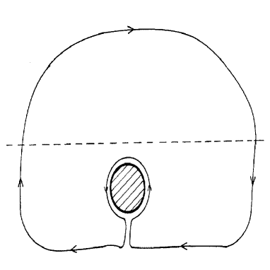
Figure 4: Magnetic field lines around a rising flux tube, with the dashed line indicating the solar surface. The flux tube, shown by the shaded circle, has magnetic field going into the paper, and it is rising in a region of clockwise poloidal field.

Now suppose a new flux tube rises to the surface and moves into the region of clockwise poloidal field. Since we are dealing with a high magnetic Reynolds number situation, the rising flux tube would not be able to cut the poloidal field lines easily and we expect that the poloidal field lines would be pushed by the rising flux tube as shown in Figure 4. Eventually the field lines left in the wake behind the flux tube would reconnect and we shall be left with an anti-clockwise twist around the flux tube. With $B_{\phi}$ inside the flux tube directed into the paper, it is easy to see that an anti-clockwise twist implies negative current helicity. If we had carried out our arguments with flux tubes having $B_{\phi}$ out of the paper (i.e. negative $B_{\phi}$), then the poloidal field lines would have been anti-clockwise and the twist around a rising flux tube clockwise, again leading to negative current helicity. When a flux tube in the northern hemisphere rises to the surface in a region of pre-existing poloidal field created by flux tubes of similar type which erupted earlier, we conclude that the flux tube acquires negative current helicity. We thus find that the observed predominant negative current helicity of active regions in the northern hemisphere has a very simple explanation within the framework of the Babcock-Leighton dynamo model. It is easy to check that our argument applied to the southern hemisphere would imply positive current helicity, in accordance with observations.

Although the current helicity of active regions in the northern hemisphere is predominantly negative, many active regions are found with positive current helicity also (Pevtsov, Canfield, and Metcalf, 1995; Abramenko, Wang, and Yurchishin, 1997; Bao and Zhang, 1998). An extremely important question is whether this is merely statistical fluctuation or whether there is some systematic aspect in it, i.e. if the positive current helicity is preferentially found in certain latitudes at certain times. More extensive data analysis will be required to settle this question. On theoretical grounds, we expect that the flux tubes may have positive current helicity systematically in certain latitudes at certain times. The argument we had given above hinges crucially on the fact that the emerging flux tube has to come up in a region where the poloidal field has been earlier created by flux tubes of the same kind, i.e. a flux tube with positive $B_{\phi}$ has to come up in a region of positive $A$. We know that flux tubes at the bottom of the convection zone are advected equatorward by the equatorward meridional flow there, whereas the poloidal field at the surface is advected poleward by the poleward meridional flow there. So, during certain phases of the solar cycle, there may be a situation in certain latitudes that $A$ at the surface has a sign which is opposite to the sign of $B_{\phi}$ of the flux tubes at the bottom of the convection zone. In such a situation, the active regions would be created with positive current helicity. A systematic study of the observed signs of current helicity in different latitudes in different phases of the solar cycle should throw important light on the nature of the solar dynamo.

6.2 Helicities at small and large scales

Now that we have seen how a rising flux tube in the northern hemisphere would pick up negative helicity, let us consider how that would appear from a mean field point of view. In a mean field approach, we average over small length scales such as the cross-section of the flux tubes. On taking average over scales larger than the flux tube cross-section, the anti-clockwise twist just outside the flux tube seen in Figure 4 would contribute zero. So we would conclude the large scale twist to be clockwise, which combined with positive $B_{\phi}$ would give us positive current helicity in the northern hemisphere. We thus find that the helicity at the large scale is opposite in sign to the helicity of flux tubes (which we consider the small scale).

It is well known that the dynamo process generates helicity. While discussing the helicity production in the dynamo process, it is more useful to think in terms of magnetic helicity ${\bf A}.{\bf B}$ rather than current helicity ${\bf j}.{\bf B}$. It is true that the definition of ${\bf A}$ is not unique due to gauge freedom and consequently there is an uncertainty in defining magnetic helicity in a local region. However, since the volume integral of magnetic helicity is connected with the topology of magnetic field (see, for example, Choudhuri, 1998), it is still an extremely useful concept, and once the gauge is fixed, we can define magnetic helicity. Unless a magnetic field has a very pathological configuration, we can normally assume that the current helicity and the magnetic helicity would have the same sign. It is easy to show that a dynamo with positive $\alpha$-effect produces positive magnetic helicity of the mean fields (Seehafer, 1996). For the benefit of the readers not very familiar with the subject, we give a simple proof in the Appendix that, in the absence of dissipation, a dynamo in a finite volume with closed field lines and with a constant $\alpha$ would generate magnetic helicity $H=\int{\bf A}.{\bf B}dV$ at the rate

$$\frac{dH}{dt}=2\alpha\int B^{2}dV,$$

clearly showing that a positive $\alpha$ implies the production of positive $H$ within the mean field framework.

Since magnetic helicity is connected with the topology of field lines, it is not possible to change the value of magnetic helicity in time scales shorter than the resistive decay time (which is very large for astronomical systems). Then how does the dynamo produce magnetic helicity of the mean field? It has been shown by Seehafer (1996) that a dynamo generates magnetic helicity at the large scales by transferring magnetic helicity of equal and opposite amount to the small scales, thus ensuring that the total amount of magnetic helicity does not change. In Figure 4 we have presented a clear physical picture of how this happens in the Babcock-Leighton framework. A positive $\alpha$ in the northern hemisphere of the Sun would produce positive helicity at the large scales and hence negative helicity at the small scales. By identifying the helicity of the flux tubes as the helicity associated with small scales, we get an understanding of why the active regions in the northern region should have predominantly negative helicity, in accordance with the observations.

6.3 The ultimate fate of helicity

A dynamo with positive $\alpha$ keeps on piling negative helicity at the small scales. If the dynamo cannot get rid of this negative helicity at the small scales, it eventually gets quenched. This is believed to be the reason for dynamo quenching found in some numerical simulations (Blackman and Field, 2000). The helicity constraint is very severe in $\alpha^{2}$ dynamos. Although it is less severe for $\alpha\Omega$ dynamos, it still has to be reckoned with (Brandenburg, Bigazzi, and Subramanian, 2001). In the CDSD models, the toroidal and the poloidal fields generated in spatially separated regions, and are not inter-linked when they are generated. The helicity is produced when toroidal flux tubes generated at the bottom of the convection zone move into regions of poloidal field, as seen in Figure 4. Still, the Sun has to get rid of the helicity continuously, to ensure that the helicity constraint does not cause any problem for the solar dynamo.

Once a flux tube emerges through the solar surface, the upper portion of it becomes a coronal loop with a cross-section much larger than that below the surface. Parker (1974) studied the magnetohydrostatic equilibrium of flux tubes with variable cross-section and showed that most of the twist would get concentrated in the region where the cross-section is maximum. Even if a solar flux tube initially had twist underneath the solar surface, after emergence through the surface the twist would presumably propagate in the form of torsional Alfven waves to be eventually concentrated in the uppermost part of the loop. Thus the negative helicity dumped by the solar dynamo at the small scales in the northern hemisphere ultimately makes its way to the upper parts of coronal loops. Magnetic filaments in the corona are indeed known to have opposite twists in the two hemispheres (Rust and Kumar, 1994). Once the twisted part of the flux tube rises through the solar surface and goes out of the convection zone, it is clear that there is no helicity left within the convection zone—either positive helicity at the large scales or negative helicity at the small scales. So there would be no problem in the convection zone arising out of the helicity constraint.

The Sun eventually has to get rid of the helicity at the tops of coronal loops by various coronal processes. If the loop becomes sufficiently twisted, it may eventually become unstable and lead to such coronal phenomena as flares or CMEs. It has been conjectured by Low (1994) that CMEs may constitute a mechanism by which the Sun gets rid of its excess helicity. It is, therefore, conceivable that the helicity of the Sun is ultimately carried away by the solar wind. When we consider the connection between the solar dynamo and the flux tubes, many different pieces of the jigsaw puzzle seem to fall in place.

7 Conclusion

To the best of our knowledge, no serious attempt has been made previously to reconcile the existence of flux tubes with the results of mean field dynamo theory. We suggest a possible procedure here: first solve the mean field dynamo equation to figure out how the mean field behaves and then use other considerations (such as results of flux tube calculations) to figure out where flux tubes would exist and what would be their nature. Only the second step is attempted in this paper, based on the solutions of CDSD model presented by various previous authors. This paper is quite unlike the other recent papers of the present author where usually detailed calculations are presented. This paper is based more on order-of-magnitude estimates and general arguments. The nature of the subject is such that it is important first to evolve a plausible scenario based on such estimates and arguments before any detailed calculation is attempted. We have, in fact, indicated a few possibilities of detailed calculations to make our picture more complete. We hope that such calculations will be done in near future.

The polar field of the Sun appears reasonably diffuse. It is not clear to what extent this field is concentrated in fibril flux tubes, but it is certainly not organized in flux concentrations as large as sunspots. In the CDSD model, this polar field is advected by the meridional circulation to the tachocline, where it is stretched to produce the strong toroidal field. Our surface observations are the following: the polar field at the time of subduction below the surface is reasonably smooth and the active regions at the time of emergence appear in the form of flux tubes. Hence the magnetic field must get organized into flux concentrations at some stage during the subsurface processes of advection of the polar field to the tachocline, the stretching by differential rotation and the subsequent rise of the toroidal field by magnetic buoyancy. Simple and straightforward considerations based on the dynamo equation conclusively rule out the possibility that the magnetic field could be smooth at the bottom of the convection zone, flux tubes breaking away from this smooth field due to some instability and rising thereafter. The polar is field is about 10 G, whereas flux tube calculations suggest that the sunspot-forming toroidal field at the bottom of the convection zone must be of order 100,000 G. An order-of-magnitude estimate shows that the differential rotation in the tachocline is not sufficient to stretch a 10 G poloidal field into a uniform 100,000 G toroidal field. From such estimates, we have been able to draw some conclusions about the volume filling factors of flux tubes.

We have suggested that the organization into flux tubes takes place while the polar field is being advected downward into the tachocline. We have estimated these flux tubes in the polar region above the tachocline to have radii of order 12,000 km and to have mean separations of order 85,000 km. Certainly not too many such flux tubes can exist at a certain time. But we expect them to be long-lived and presumably some of these flux concentrations eventually become active regions after a few years, after being stretched in the toroidal direction in the tachocline while they are advected to lower latitudes. Our estimate of filling factor should be of interest to helioseismologists who are looking for signatures of magnetic field at the bottom of the convection zone. In a decade or two, perhaps the techniques of helioseismology may become sophisticated enough to study the formation of flux tubes above the tachocline and then follow them as they get titled in the toroidal direction and are advected to lower latitudes, eventually to emerge as active regions. The model of Nandy and Choudhuri (2002) imply that the active regions could not be like tips of icebergs, constituting a small part of the toroidal field sitting at the bottom of the convection zone. Rather, all the toroidal flux at the bottom of the convection zone has to come up when the penetrating meridional flow rises. This solves the mystery of how the strong 100,000 G field gets annihilated in 11 years. We also point out that the intermittent nature of the magnetic field in the tachocline makes it possible for the meridional flow to advect it to the lower latitudes, without being resisted by the magnetic tension or the Coriolis force.

The major uncertainty in our scenario is that we do not understand what determines the lengths of toroidal flux concentrations at the bottom of the convection zone. We have suggested that the horizontal widths of plumes penetrating below the bottom may have something to do with this. Perhaps a numerical simulation to study how the magnetic configuration shown in Figure 2 would get advected into the tachocline by intermittent plumes would throw more light on this question.

During the last decade, considerable work has been done on the current helicities of active region. Our model gives a disarmingly simple explanation of the observed current helicity. Flux tubes from the bottom of the convection zone rise to the region where there exists a poloidal field created by similar flux tubes earlier and they get a twist in this process. This explanation matches the sign of the observed current helicity. A fundamental question in dynamo theory is the relation between helicities at large and small scales, as well as the ultimate fate of the helicity. When we combine flux tube considerations with considerations of dynamo theory, we seem to get very natural answers to some of these intriguing questions.

Appendix. Magnetic helicity generation in dynamo process

We consider dynamo action in a volume bounded by a surface through which fluid elements or magnetic field lines do not pass (i.e. both ${\bf v}$ and ${\bf B}$ on the boundary are zero). Let the $\alpha$ coefficient be constant within this volume and let the diffusion coefficient be zero. Then the dynamo equation is given by

$$\frac{\partial{\bf B}}{\partial t}=\nabla\times({\bf v}\times{\bf B})+\nabla\times(\alpha{\bf B}).$$

We choose the gauge of the vector potential such that it satisfies the equation

$$\frac{\partial{\bf A}}{\partial t}={\bf v}\times{\bf B}+\alpha{\bf B}.$$

The rate of change of the magnetic helicity $H=\int{\bf A}.{\bf B}dV$ is given by

$$\frac{dH}{dt}=\int\frac{\partial{\bf A}}{\partial t}.{\bf B}\,dV+\int{\bf A}.\frac{\partial{\bf B}}{\partial t}\,dV.$$

On substituting from (15) and (16), we get

$$\frac{dH}{dt}=\alpha\int B^{2}\,dV+\int{\bf A}.[\nabla\times({\bf v}\times{\bf B}+\alpha{\bf B})]\,dV.$$

The second integral on the right hand side can be written in the following way

$$\int({\bf v}\times{\bf B}+\alpha{\bf B}).\nabla\times{\bf A}\,dV-\int\nabla.[{\bf A}\times({\bf v}\times{\bf B}+\alpha{\bf B})]\,dV.$$

The second term here is a volume integral of a divergence and can be converted into a surface integral by Gauss’s theorem. It is easy to see that this term would vanish if ${\bf v}$ and ${\bf B}$ are zero on the surface. Remembering that $\nabla\times{\bf A}={\bf B}$, we note that the first term in (18) gives $\alpha\int B^{2}dV$. It then follows from (17) that

$$\frac{dH}{dt}=2\alpha\int B^{2}\,dV.$$

We thus see that dynamo action generates magnetic helicity having the same sign as $\alpha$.

References

Abramenko, V. I., Wang, T., and Yurchishin, V.B.: 1997, Solar Phys. 174, 291.

Babcock, H. W.: 1961, Astrophys. J. 133, 572.

Bao, S. and Zhang, H.: 1998, Astrophys. J. 496, L43.

Blackman, E. G. and Field, G. B.: 2000, Astrophys. J. 534, 984.

Bonanno, A., Elstner, D., Rüdiger, G., and Belvedere, G.: 2002, Astron. Astrophys. 390, 673.

Brandenburg, A., Bigazzi, A., and Subramanian, K.: 2001, Mon. Notic. Roy. Astron. Soc. 325, 685.

Braun, D. L. and Fan, Y.: 1998, Astrophys. J. 508, L105.

Caligari, P., Moreno-Insertis, F., and Schüssler, M.: 1995, Astrophys. J. 441, 886.

Charbonneau, P. and MacGregor, K. B.: 1997, Astrophys. J. 486, 502.

Choudhuri, A. R.: 1989, Solar Phys. 123, 217.

Choudhuri, A. R.: 1998, The Physics of Fluids and Plasmas: An Introduction for Astrophysicists, Cambridge University Press.

Choudhuri, A. R.: 2002, in B. N. Dwivedi (ed.), The Dynamic Sun, Cambridge University Press, p. 103.

Choudhuri, A. R. and Dikpati, M.: 1999, Solar Phys. 184, 61.

Choudhuri, A. R. and Gilman, P. A.: 1987, Astrophys. J. 316, 788.

Choudhuri, A. R., Schüssler, M., and Dikpati, M.: 1995, Astron. Astrophys. 303, L29.

Dikpati, M. and Charbonneau, P.: 1999, Astrophys. J. 518, 508.

Dikpati, M. and Choudhuri, A. R.: 1994, Astron. Astrophys. 291, 975.

Dikpati, M. and Choudhuri, A. R.: 1995, Solar Phys. 161, 9.

Dikpati, M. and Gilman, P. A.: 2001, Astrophys. J. 559, 428.

D’Silva, S. and Choudhuri, A. R.: 1993, Astron. Astrophys. 272, 621.

D’Silva, S. and Howard, R. F.: 1993, Solar Phys. 148, 1.

Durney, B. R.: 1995, Solar Phys. 160, 213.

Durney, B. R.: 1996, Solar Phys. 166, 231.

Durney, B. R.: 1997, Astrophys. J. 486, 1065.

Durney, B. R.: 2000, Astrophys. J. 528, 486.

Fan, Y., Fisher, G. H., and DeLuca, E. E.: 1993, Astrophys. J. 405, 390.

Ferriz-Mas, A., Schmitt, D., and Schüssler, M.: 1994, Astron. Astrophys. 289, 949.

Giles, P. M., Duvall, T. L., and Scherrer, P. H.: 1997, Nature 390, 52.

Gilman, P. A.: 1983, Astrophys. J. Suppl. 53, 243.

Glatzmaier, G. A.: 1985, Astrophys. J. 291, 300.

Küker, M., Rüdiger, G., and Schultz, M.: 2001, Astron. Astrophys. 374, 301.

Leighton, R. B.: 1969, Astrophys. J. 156, 1.

Longcope, D. and Choudhuri, A. R.: 2001, Solar Phys. 205, 63.

Longcope, D. and Fisher, G. H.: 1996, Astrophys. J. 458, 380.

Longcope, D., Fisher, G. H., and Pevtsov, A. A.: 1998, Astrophys. J. 507, 417.

Low, B. C.: 1994, Phys. Plasmas 1, 1684.

Miesch, M. S., Elliott, J. R., Toomre, J., Clune, T. L., Glatzmaier, G. A., and Gilman, P. A.: 2000, Astrophys. J. 532, 593.

Moffatt, H. K.: 1978, Magnetic Field Generation in Electrically Conducting Fluids, Cambridge University Press.

Moreno-Insertis, F.: 1983, Astron. Astrophys. 122, 241.

Moreno-Insertis, F.: 1986, Astron. Astrophys. 166, 291.

Nandy, D. and Choudhuri, A. R.: 2001, Astrophys. J. 551, 576.

Nandy, D. and Choudhuri, A. R.: 2002, Science 296, 1671.

Parker, E. N.: 1955, Astrophys. J. 122, 293.

Parker, E. N.: 1974, Astrophys. J. 191, 245.

Parker, E. N.: 1975, Astrophys. J. 198, 205.

Parker, E. N.: 1979, Cosmical Magnetic Fields, Oxford University Press.

Parker, E. N.: 1993, Astrophys. J. 408, 707.

Pevtsov, A. A., Canfield, R. C., and Latushko, S. M.: 2001, Astrophys. J. 549, L261.

Pevtsov, A. A., Canfield, R. C., and Metcalf, T. R.: 1995, Astrophys. J. 440, L109.

Rust, D. M. and Kumar, A.: 1994, Solar Phys. 155, 69.

Seehafer, N.: 1990, Solar Phys. 125, 219.

Seehafer, N.: 1996, Phys. Rev. E 53, 1283.

Steenbeck, M., Krause, F., and Rädler, K.-H.: 1966, Z. Naturforsch. 21a, 1285.

van Ballegooijen, A. A. and Choudhuri, A. R.: 1988, Astrophys. J. 333, 965.

Wang, Y.-M., Nash, A. G., and Sheeley, N. R.: 1989, Astrophys. J. 347, 529.