Constraints on the Ionization Balance of Hot-Star Winds from FUSE Observations of O Stars in the Large Magellanic Cloud

Abstract

We present Far Ultraviolet Spectroscopic Explorer (FUSE) spectra for 25 O stars in the Large Magellanic Cloud (LMC). We analyze wind profiles for the resonance lines from C iii, N iii, S iv, P v, S vi, and O vi in the FUSE range using a Sobolev with Exact Integration (SEI) method. In addition, the available data from either IUE or HST for the resonance lines of Si iv, C iv, and N v are also modeled. Because several of the FUSE wind lines are unsaturated, the analysis provides meaningful optical depths (or, equivalently, mass loss rate times ionization fractions, $\dot{M}q$), as a function of normalized velocity, $w=v/$${v}_{\infty}$. Ratios of $\dot{M}q$ (which are independent of $\dot{M}$) determine the behavior of the relative ionization as a function of $w$. The results demonstrate that, with the exception of O vi in all stars and S vi in the later stars, the ionization in the winds shifts toward lower ionization stages at higher $w$ (contrary to the expectations of the nebular approximation). This result implies that the dominant production mechanism for O vi and S vi in the late O stars differs from the other ions.

Using the Vink et al. (2001) relationship between stellar parameters and mass-loss rate, we convert the measurements into mean ionization fractions for each ion, $\langle q_{i}\rangle$. Because the derived ion fractions never exceed unity, we conclude that the derived values of $\dot{M}$ are not too small. However, $q$(P v), which is expected to be the dominant stage of ionization in some of these winds, is never greater than 0.20. This implies that either the calculated values of $\dot{M}$ are too large, the assumed abundance of phosphorus is too large or the winds are strongly clumped. The implications of each possibility are discussed. Correlations between the mean ion fractions and physical parameters such as $T_{\rm eff}$, ${v}_{\infty}$ and the mean wind density, $\langle\rho\rangle$ are examined. Two clear relationships emerge. First, as expected, the mean ionization fraction of the lower ions C iii, N iii, Si iv, S iv) decreases with increasing $T_{\rm eff}$. Second, the mean ion fraction of S vi in the latest stars and O vi in all stars increases with increasing ${v}_{\infty}$. This re-affirms the notion, first introduced by Cassinelli & Olson (1979), that O vi is produced non-radiatively.

Finally, we discuss specific characteristics of three stars, BI 272, BI 208, and Sk $-67{{}^{\circ}}166$. For BI 272, the ionic species present in its wind suggest a much hotter than its available (uncertain) spectral type of O7: II-III:. In the case of BI 208, our inability to fit its observed profiles suggests that its wind is not spherically symmetric. For Sk $-67{{}^{\circ}}166$, quantitative measurements of its line strengths confirm the suggestion by Walborn et al. (1995) that it is a nitrogen rich O star.

1 Introduction

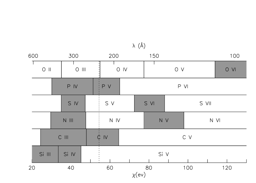
Figure 1: Schematic representation of the range in ionization spanned by ions that produce stellar wind lines in spectra of O-type stars. Ions in shaded boxes are those with observed resonance lines, while ions in unshaded boxes do not have resonance lines in the FUV or UV. Open-ended boxes indicate that the ion persists beyond the range of the plot. The dashed vertical line indicates the ionization potential of He ii, 54.4 eV. Ions that lie completely to the right of this line are “super-ions,” i.e., ions that cannot be abundantly produced by photoionization from the ground state, since the stellar continuum flux shortward of 228 Å is drastically reduced by bound-free absorption from He ii.

Although the stellar winds of early-type stars are understood to be driven by momentum transfer from the underlying stellar radiation field, there is overwhelming evidence that the ionization conditions in the wind are not solely determined by radiative processes. Initial indications for the influence of additional processes came from observations of wind profiles for “super-ions” like N v and O vi by the Copernicus observatory (see, e.g. Snow & Morton, 1976; Walborn & Bohlin, 1996). Figure 1 is a schematic representation of the ionization ranges of the ions whose wind lines are analyzed in this paper as well as those ions which do not have observable lines. The dashed vertical line denotes the ionization potential of He ii. Ions which lie completely to the right of this line are super-ions. The abundances of super-ions are expected to be quite low in all but the hottest stars, since direct photoionization of the ground state of the next lower ion should be rare. This is because the flux of photons sufficiently energetic to create them is strongly suppressed by bound-free absorption of He⁺ in the photosphere. However, the strength of the super-ion wind lines and, especially, the presence of O vi, lead Cassinelli & Olson (1979) to predict that hot-star winds must emit X-rays, which could then modify the abundances of super-ions via Auger ionization. This prediction was subsequently confirmed by observations from the Einstein (Harnden et al., 1979; Seward et al., 1979; Chlebowski et al., 1989), ROSAT (Berghöfer et al., 1996) and ASCA observatories (Corcoran et al., 1994). More recent observations with the spectrometers onboard Chandra and XMM-Newton indicate the presence of even more highly ionized species (see, e.g., Schulz et al., 2000; Kahn et al., 2001; Waldron & Cassinelli, 2001; Cassinelli et al., 2001).

The origin of X-rays in hot-star winds is still an open issue. Shocks due to the intrinsic line-driven instability (Owocki et al., 1988) or the formation of large-scale, co-rotating structures (Cranmer & Owocki, 1996) or heating of plasma in a magnetic loops (ud-Doula & Owocki, 2002) are likely possibilities, while models invoking the presence of a deep-seated, hot corona (e.g., Cassinelli & Olson, 1979; Waldron, 1984) are not considered as plausible. Since their origin is so uncertain, X-rays are included in the current generation of model atmospheres only in an ad hoc manner (see, e.g., Hillier & Miller, 1998; Pauldrach et al., 1994, 2001). Predicted ionization equilibria from model atmosphere calculations are further complicated by uncertainties in the treatment of line blocking and blanketing in the far- and extreme-ultraviolet regions of the spectrum, which determine the flux of hard photospheric photons that are available to illuminate the wind. Thus, despite the impressive progress in calculating sophisticated ab initio models of moving atmospheres reviewed recently by Kudritzki & Puls (2000), self-consistent theoretical determinations of the prevailing ionization conditions remain elusive.

Theoretical progress is further complicated by the limited guidance provided by observations. Essentially all empirical information concerning the ionization of the wind material comes from observations of the ultraviolet (UV) resonance lines of ionized metals, which are the most sensitive indicators of mass loss. By modeling the wind profiles of these species, it is possible to determine the radial optical depth (or equivalently, column density) of the ion as a function of velocity in the stellar wind. Since the degree of excitation for metal ions is extremely low, this can be expressed directly in terms of the product of the mass-loss rate and ionization fraction, $\dot{M}q$, for the species (e.g.,  Hamann, 1980, 1981; Lamers et al., 1987; Groenewegen & Lamers, 1989; Howarth & Prinja, 1989; Groenewegen & Lamers, 1991). However, the resonance lines of abundant elements, and especially the dominant ionization stages of these elements, are often saturated, and provide only lower limits on the quantity of the ion in the wind. The spectral diagnostics accessible to IUE and HST – usually N v $\lambda\lambda$1239, 1243, Si iv $\lambda\lambda$1394, 1403, and C iv $\lambda\lambda$1548, 1551 – are especially problematical, since C and N are cosmically abundant and hence frequently saturated. Furthermore, even when two or more of these lines are unsaturated ratios of their respective values of $\dot{M}q_{i}$ still depend on the abundance of their parent element. The abundance of C and N can differ substantially from nominal values in the atmospheres of OB stars, particularly supergiants, due to mixing of material processed through the CNO cycle from the interior. Thus, even the ratios of ion fractions are difficult to interpret from these diagnostics, unless the actual abundances of C and N have been determined by some means.

In contrast, the far-ultraviolet (FUV; $\sim$905–1215 Å) region provides a much richer suite of resonance line diagnostics. As detailed in §4, these include (a) lines from cosmically abundant (e.g., O, C, N) and comparatively rare (e.g., S, P) elements, which are less likely to be saturated; (b) lines from species that are expected to dominant (e.g., P v) and trace (e.g, C iii) ions; (c) lines from multiple ionization stages of the same element (e.g., S iv/S vi); and (d) lines from super-ions (e.g., S vi and O vi) and low ions (e.g., N iii). Many of the earliest measurements of resonance lines in the winds of early-type stars were based on FUV observations obtained by Copernicus; see, e.g., Gathier et al. (1981) and Olson & Castor (1981). However, due to the severity of interstellar extinction and limited instrumental sensitivity, spectra below 1000 Å were obtained for an extremely limited sample of Galactic O and early B-type stars, most notably $\zeta$ Puppis (O4 In(f); Morton & Underhill, 1977) and $\tau$ Scorpii (B0 V; Rogerson & Upson, 1977). As a result, these two objects have dominated theoretical modeling efforts for the last two decades, particularly those aimed at tracing the distribution of the X-rays believed responsible for superionization (e.g., MacFarlane et al., 1993).

With the launch of the Far Ultraviolet Spectroscopic Explorer (FUSE) in 1999 June, routine access to the FUV region of the spectrum has become available once more. Unlike Copernicus, FUSE is sensitive enough to provide high signal-to-noise (S/N), high resolution spectra of O-type stars in the Large and Small Magellanic Clouds (LMC and SMC). Furthermore, in contrast to the sensitive, high-resolution FUV spectrographs flown in the on shuttle-based missions in the mid-1990s (particularly the Berkeley Extreme and Far Ultraviolet Spectrometer), the duration of the FUSE mission permits extensive surveys of the hot stars in these galaxies. Access to OB-type stars in the Magellanic Clouds provides several distinct advantages over previous work.

First, early-type stars in the LMC and SMC are only lightly reddened, especially when compared with Galactic O stars that are faint enough to be observed by FUSE (i.e., $F_{\lambda}\leq 1\times 10^{-10}$ erg s^-1 cm^-2 Å^-1 throughout the FUV region). As a result, their continuum flux distributions are nearly flat over the entire FUV waveband, and problems caused by blending of stellar features with interstellar absorption lines are more manageable than in most of their Galactic counterparts. Thus, FUSE observations of early-type stars in the Magellanic Clouds provide the first systematic assessment of the behavior of the important stellar wind diagnostics below 1000 Å, particularly the resonance lines of S vi, P iv, C iii, and N iii. These trends are described and illustrated in the detailed atlas of FUSE spectra prepared by Walborn et al. (2002a).

Second, since the abundance of metals in the Magellanic Clouds is smaller than in the Milky Way, the effect of metallicity on the bulk properties of stellar winds can be probed. The hot stars in each of the Magellanic Clouds lie at a common, known distance and are thought to be a members of a homogeneous population. Consequently, the Magellanic Clouds are ideal laboratories for studying the physics of line-driven stellar winds. Initial analyses of FUSE spectra have been reported by Bianchi et al. (2000), who performed wind-profile fitting for a matched pair of O supergiants (one from each Cloud) and Fullerton et al. (2000), who used model atmospheres to estimate the stellar parameters for the same objects.

In this paper, we present the first comprehensive investigation of the properties of the stellar winds of O-stars in the LMC at FUV wavelengths. In particular, we use measured optical depths in various resonance lines and assumed mass-loss rates to determine empirical ionization fractions, which provide qualitatively new information about the ionization balance in the winds of these stars. §2 provides a description of the program stars, the observations, and the data processing, while §3 describes the wind-profile fitting technique used to characterize the properties of the outflows. Characteristics of the resonance lines analyzed are given in §4, which also includes a discussion of specific problems associated with fitting them. The results of the measurements and their errors are described in §5 and discussed in §6. The conclusions are summarized in §7.

2 Observations and Data Processing

2.1 Program Stars

The sample of O stars presented here was largely drawn from programs designed by the FUSE Principal Investigator team to study the stellar content and interstellar medium (ISM) of the LMC. The sample represents a subset of the data available in late 2001, which was selected to provide full coverage of the O-type temperature classes with minimal reddening. Stars known to be members of complicated binary systems were avoided, and stars with bright neighbors that fell within the FUSE large aperture were also eliminated. A secondary criterion was that the targets should also have spectra covering the UV resonance lines in the $1200\leq\lambda\leq 1700$ Å region from either high dispersion IUE, HST / FOS, or HST / STIS observations. Archival spectra from one or more of these sources were available for all but two targets (Sk $-67{{}^{\circ}}69$ and Sk $-70{{}^{\circ}}115$).

Table 1 lists the fundamental properties of the 25 stars in our sample. Successive columns record the designations of the objects in the catalogs of either Sanduleak (1970, Sk) or Brunet et al. (1975, BI); commonly used aliases; the spectral classification and its source; the terminal velocity (${v}_{\infty}$) of the wind as determined by the current investigation; the adopted effective temperature ($T_{\rm eff}$) from the spectral-type – $T_{\rm eff}$ calibration of Vacca et al. (1996); the computed stellar luminosity; and the adopted mass-loss rate ($\dot{M}$). Table 2 lists the optical data ($V$ and B V) and their origin, the derived $E$(B V), the observed FUV flux value at the fiducial wavelength 1150 Å  and the identifications of the FUSE observations, IUE, or HST data sets used.

The stellar luminosities in Table 1 were calculated using the the Vacca et al. (1996) bolometric corrections, $BC$, for the adopted $T_{\rm eff}$, the observed $V$ magnitude given in Table 2, corrected for extinction (using the spectral type – (B V)₀ calibration of FitzGerald (1970) and a total-to-selective extinction ratio of $R(V)=A(V)/E(B-V)=3.1$) and an adopted LMC distance modulus ($DM$) of 18.52 (Fitzpatrick et al., 2002). Deviations from the assumed value of $R(V)$ have little effect on the luminosity, since the reddenings are quite modest.

The mass-loss rates in Table 1 were estimated from the adopted stellar parameters by using the relationship derived by Vink et al. (2000,  their eq. [15])

$$\log\dot{M}=-15.88+1.576\log L/L_{\sun}+\log T_{\rm eff}-\log v_{\infty}$$ (1)

These estimates were further adjusted to account for the lower metallicity of the LMC by means of the scaling relation

$$\log\dot{M}=\log\dot{M}+0.69\log Z/Z_{\sun}$$ (2)

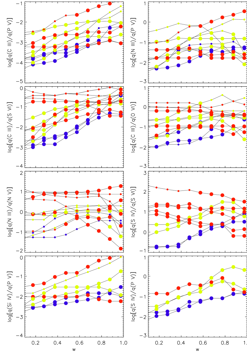
Figure 6: Ratios of ion fractions as a function of normalized velocity, $w$, for the species specified on the ordinates. The ratios are always specified with the higher ion as the denominator. Ratios containing saturated points are shown as small symbols. Data for all stars are overplotted, with different symbols representing the temperature ranges as follows – red: $T_{\rm eff}$ $\leq$ 38 kK; yellow: 38 $<$ $T_{\rm eff}$ $\leq$ 45 kK; blue: $T_{\rm eff}$ $>$ 45 kK.

from Vink et al. (2001), where we adopt $Z/Z_{\sun}=0.5$ for the LMC (Rolleston et al., 1996; Welty et al., 1995). This value lies between the extremes examined by Vink et al. and provides good agreement between their predicted mass loss rates and those observed by Puls et al. (1996) (see Figure 6 in Vink et al.).

Insofar as Vacca et al. (1996), Vink et al. (2001) and Puls et al. (1996) used similar temperature calibrations, we expect the estimates of $\dot{M}$ to be internally consistent. Accordingly, the random uncertainty in $\dot{M}$ is dominated by the uncertainties in $T_{\rm eff}$, $\log L/L_{\sun}$ and $\log Z/Z_{\sun}$. The effective temperature of a program star cannot be known better than half a spectral class, which corresponds to $\sim 1.5$ kK for a typical O star temperature of 40 kK (Vacca et al. 1996). This error enters the $\dot{M}$ determination both explicitly and implicitly through its effect on the $BC$ which is used to determine the luminosity; specifically, $\log L/L_{\odot}=-0.4(M_{V}+BC-M_{bol,\odot})$. Since $M_{V}$ is constrained by the adopted distance to the LMC, the only error in $\log L/L_{\odot}$ is due to the temperature uncertainty in their $BC$. A typical half spectral class change in the $BC$ is $-0.1$, which translates into $+0.04$ in $\log L/L_{\odot}$. Thus, for typical O star values, a $\log\dot{M}$ error due to the expected uncertainty in $T_{\rm eff}$ is $1.576(0.04)-\log(1+1500/40000)\sim 0.05$, or 12%. Another error results from the uncertainty in the LMC distance, which is at least $\pm 0.1$ in the distance modulus, which corresponds to an error of $1.576\times 0.4\times 0.1$ in $\log\dot{M}$, or about 15% in $\dot{M}$. Finally, $\log Z/Z_{\sun}$ is not known to better than 20%, and this error propagates to 14% in $\dot{M}$. Now, if we assume that each of these errors (due to temperature, LMC distance and abundances) are independent, then (as long as the Vink et al. relations are exact), the overall uncertainty in the derived $\dot{M}$ values should be less than 25%.

2.2 Far Ultraviolet Spectra

The FUSE observatory consists of four aligned, prime-focus telescopes, and Rowland-circle spectrographs that feed two photon-counting detectors. Two of the telescope/spectrograph channels have SiC coatings to cover the range $\sim 905-1105$ Å, while the other two have LiF coatings to cover the $\sim 980-1188$ Å with high throughput. These are referred to as the SiC and LiF channels, respectively. Each channel has its own focal plane assembly, which contains three entrance apertures of different sizes. After passing through one of these apertures, light is diffracted and focused by the concave gratings onto a delay-line detector, each of which records a pair of (SiC, LiF) spectra. For faint objects, the detectors are operated in “time-tag” mode to record the arrival time and detector position of individual photon events; for brighter sources, the incoming photons are recorded in “histogram” mode, which only retains positional information. Since each detector is subdivided into two segments (labeled “A” and “B”), eight independent spectra are ultimately obtained, one for each combination of channel and detector segment. As a result, nearly the entire wavelength range between 905 and 1187 Å is redundantly covered by at least two independent spectra. Further details of the FUSE mission, its instrumentation, and in-orbit performance are provided by Moos et al. (2000) and Sahnow et al. (2000b).

The observations presented here were obtained between 1999 December 15 and 2000 December 4, during the first year of the prime mission of FUSE. All observations were made through the large, $30{\arcsec}\times 30{\arcsec}$ (LWRS) aperture in time-tag mode, with typical integration times of $\sim$8 ks. Although thermal motions of the telescope mirrors causes channel misalignment, the targets always remained in the LWRS apertures and no data were lost.

The spectra were processed uniformly with version 1.8.7 of the standard calibration pipeline software package, CALFUSE. Processing steps included application of corrections for small, thermally-induced motions of the diffraction gratings; removal of detector backgrounds; correction for thermal and electronic distortions in the detectors; extraction of a one-dimensional spectrum by summing over the astigmatic height of the two-dimensional image; correction for the minor effects of detector dead time; and application of flux and wavelength calibrations. CALFUSE 1.8.7 did not include corrections for residual astigmatism in the spectrograph or fixed-pattern noise in the detector, which limit the spectral resolution and S/N ratio of the extracted spectra, respectively. Neither of these omissions are detrimental to this program, since analysis of wind profiles does not require extremely high spectral resolution, and since we always compared redundant data from different channels to determine the reality of weak spectral features.

However, the data were adversely affected by an anomaly known as “the worm,” which is a region of depressed flux caused by shadowing from grid wires located near the detector to enhance its quantum efficiency (Sahnow et al., 2000a). The most severe worm affects the longest wavelength regions of spectra from the LiF1 channel recorded by detector segment B. Fortunately, we were able to use the redundant information from LiF2 channel (detector segment A) to recover the true shape of the longest wavelength lines in our study (P v $\lambda\lambda$1118, 1128).

Finally, the fully processed spectra, which have a nominal spectral resolution of $\sim$20 km s^-1 (FWHM), were smoothed to a resolution of $\sim$30 km s^-1 in order to enhance the S/N ratio. Due to errors in the wavelength scale of CALFUSE 1.8.7, we found that systematic velocity shifts of about $-50$ km s^-1 were required to place the strong interstellar H₂ lines due to absorption in the Milky Way at zero velocity. The magnitude and sense of this shift agrees with the results of Danforth et al. (2002) and Howk et al. (2002), who considered the problem in greater detail.

2.3 Ancillary UV Spectra

Fully processed, archival data sets of the targets obtained by IUE or HST were retrieved from the Multimission Archive at Space Telescope (MAST). The specific data sets are listed in Table 2. These spectra were subsequently smoothed in order to enhance their S/N. STIS spectra were smoothed to an effective resolution of 30 km s^-1 in order to match the FUSE data, while the high dispersion IUE spectra (which were typically of quite poor quality at full resolution) were smoothed to 60 km s^-1 to increase the S/N ratio. The FOS spectra were smoothed by 100 km s^-1, which is less than their intrinsic resolution of $\sim 240$ km s^-1.

3 Wind Profile Analysis

3.1 Overview

The shapes of P Cygni wind profiles of resonance lines encode information about the velocity law governing the expansion of the wind; any additional macroscopic velocity fields that might be present, e.g., due to shocks; the abundance and distribution of the parent ion; and the total amount of material in the wind. This information can be accessed by fitting the profiles subject to an underlying model for the structure of the wind. Indeed, self-consistent fits are the only way to extract information about the velocity law and ionic column densities as a function of velocity in the wind. This information is especially useful when several stars (or observations of the same star obtained over several epochs) are analyzed together, since any limitations of the underlying wind model are compensated to some extent by differential analysis of the trends exhibited by different ions. Previous work based on IUE spectra of O-type stars by Howarth & Prinja (1989), Groenewegen & Lamers (1989; 1991), Haser (1995) and Lamers et al. (1999) demonstrate the utility of this approach.

We employed a modified version of the “Sobolev with Exact Integration” (SEI) computer program developed by Lamers et al. (1987) together with a simplified model of the interstellar H i and H₂ along the line of sight, to obtain precise fits to the P Cygni profiles in the FUSE and IUE/HST wavebands. These fits yielded measurements of the run of wind optical depths as a function of velocity for the ion analyzed. These were subsequently converted into the product of mass-loss rate and ionization fraction, $\dot{M}q_{i}$$(v)$. Finally, we used the Vink et al. (2000; 2001) formulae for mass-loss rates to convert the $\dot{M}q_{i}$$(v)$ measurements into velocity-dependent ionization fractions for each observed ion, $q_{i}(v)$. The following sub-sections describe the details of this procedure.

3.2 The SEI Method

The SEI method computes wind profiles for homogeneous, spherically symmetric stellar winds characterized by smoothly accelerating velocity laws. It accounts fully for blending between the components of closely spaced doublets. The inputs are specified in the following way.

Terminal Velocity. A determination of ${v}_{\infty}$ is required to compute the normalized velocity parameter $w\equiv v(r)/$${v}_{\infty}$.

Velocity Law. We assume a standard “$\beta$-law” for the expansion of the wind, which has the form

$$w=w_{0}+(1-w_{0})(1-1/x)^{\beta},$$ (3)

where $x=r/R_{\star}$ and $R_{\star}$ is the stellar radius (Lamers et al., 1987). We set $w_{0}=0.01$ in all cases. The value of $\beta$ selected affects the overall shape of the profile, since it governs the density distribution, $\rho(x)$, through the equation of mass continuity:

$${\dot{M}}=4\pi R_{\star}^{2}v_{\infty}x^{2}w(x)\,\rho(x)~{}.$$ (4)

Since $w$ is a monotonically increasing function of $x$ and the geometry is assumed to be spherically symmetric, there is a one-to-one mapping between velocity and radial position in the wind.

The parameters of the velocity law are usually determined from a saturated wind line. Profiles produced by small $\beta$ values ($\sim 0.5$) have shallower and broader red emission peaks than profiles with larger $\beta$ values. The reason is that low $\beta$ winds accelerate more rapidly. As a result, more of the low speed, red-shifted wind material is occulted by the stellar disk.

Turbulent Velocity. The turbulent velocity field is characterized by a Gaussian distribution, which is specified by the 1$\sigma$ dispersion parameter $w_{D}$. This additional dispersion is intended to simulate the effects of macroscopic velocity fields due, e.g., to shocks in the wind, on the line profile. It effectively smooths the distribution of optical depth as a function of $w$, which causes saturated portions of strong P Cygni profiles to be extended by a few times $w_{D}$. Its primary effects are to decrease the sharpness of the absorption trough near ${v}_{\infty}$ and shift the maximum velocity seen in absorption blueward, and to shift the strength of the emission peak redward. The latter effect is an artifact of the assumed constancy of $w_{D}$ throughout the wind, which usually implies that extremely large - and probably aphysical - velocity dispersions are present deep in the stellar wind; see, e.g., Haser (1995; 1998) for discussion of this point. In practice, use of a constant $w_{D}$ has little effect on subsequent analysis, since optical depths close to $w=0$ are excluded from consideration.

Input Photospheric Spectrum. In the absence of reliable templates for the wind-free FUV and UV flux distributions of O-type stars, we assumed that the continuum was either flat (i.e., no photospheric absorption lines corresponding to the resonance lines under consideration) or that the photospheric profiles were free parameters given by Gaussian distributions of optical depth

$$r_{w}=\exp\{-\tau_{0}^{B}\exp[-w^{2}/\sigma_{w}^{2}]-\tau_{0}^{R}\exp[-(w-\delta_{w})^{2}/\sigma_{w}^{2}]\},$$ (5)

where $\tau_{0}^{R}/\tau_{0}^{B}=f_{R}/f_{B}$, the ratio of oscillator strengths for the doublet (or zero for a singlet); $\delta_{w}$ is the spacing of the doublet in normalized velocity; and $\sigma_{w}$ is related to the full width of the line expressed as a velocity, $v_{G}$, by $v_{G}=2\sqrt{\ln 2}\sigma_{w}v_{\infty}$. Strengthening the photospheric spectrum affects the P Cygni profile near $w=0$ by increasing the strength of the absorption trough and decreasing the strength of the emission lobe.

Optical Depth of the Wind. The optical depth of the wind is assumed to be given by the radial Sobolev optical depth, $\tau_{rad}$$(w)$, which we modeled in a set of 21 independent velocity bins whose magnitudes were adjusted to obtain the best fit. This approach has been used previously by Massa et al. (1995b), and is similar to the technique described by Haser (1995). It has the advantage of avoiding biases due to preconceived notions about the functional form of the distribution of $\tau_{rad}$$(w)$. It also simplifies the fitting procedure, since $\tau_{rad}$$(w)$ is the only free parameter once the velocity law and photospheric spectrum are fixed. This fitting scheme relies on the fact that in a monotonically expanding, spherically symmetric outflow, only material with $w\leq w_{i}+w_{D}$ contributes to the formation of the line profile at $w_{i}$; see, e.g., the discussion of P Cygni profile formation in Lamers & Cassinelli (1999). Therefore, the profiles can be fit by first determining the value of $\tau_{rad}$$(w)$ that fits the profile at $w\approx 1$, and then stepping inward through the absorption trough (see Massa et al., 1995b). At each step $i$, the value of $\tau_{rad}$$(w_{i})$ is changed until a satisfactory fit to the profile at $w_{i}$ is achieved. As long as the fundamental assumptions of the model are correct, particularly a monotonicity of the velocity law and spherical symmetry, reliable values of $\tau_{rad}$$(w)$ are derived.

Ion Fractions. While $\tau_{rad}$ determines the shape of the profile, the more physically meaningful quantity is the ionization fraction, $q_{i}(w)$. The ionization fraction is related to $\tau_{rad}$ by (see, e.g., Olson, 1982)

$$q_{i}(w)=\left(\frac{m_{e}c}{\pi e^{2}}\right)\frac{4\pi\mu m_{H}}{f\lambda_{0}A_{E}}\frac{R_{\star}v_{\infty}^{2}}{\dot{M}}x^{2}w\frac{dw}{dx}\tau_{rad}(w)$$ (6)

where $q_{i}(w)$ is the fraction of element $E$ in ionization state $i$ at velocity $w$; $\dot{M}$ is the mass-loss rate of the star; $\mu$ is the mean molecular weight of the plasma (which was set to 1.35 for all program stars); $A_{E}$ is the abundance of element $E$ relative to hydrogen by number and all other symbols have their usual meaning. Adopted values of the oscillator strengths and elemental abundances are given in Table 3.

3.3 Procedure to Fit Wind Profiles

FUSE spectra are affected by a wealth of interstellar absorption lines, which include numerous H₂ lines, the upper Lyman series of H i, and several strong lines from metallic ions such as O i, N i, C ii, and Si ii (see, e.g., Friedman et al., 2000). As a result, the FUV spectrum of even a lightly reddened star is strongly affected by ISM lines which complicates the analysis considerably (see Bianchi et al., 2000; Fullerton et al., 2000). This plethora of strong interstellar lines throughout the FUSE range affects the analysis in two respects. First, a rough model of the ISM absorption is required in to disentangle the effects of stellar and interstellar absorption. Second, the resulting complexity of the spectrum makes any automated fitting scheme effectively impossible. Consequently, all fits were performed interactively.

The first step of the analysis for each star was to estimate interstellar H i and H₂ column densities from interactive fits of a simple model to the observed interstellar lines. The model consisted of two H i components, one appropriate to the Galaxy and one appropriate to the LMC, and a single component for Galactic H₂. For the H₂ model, we fit each rotational level with its own column density and velocity spread parameter (i.e., $b$-value). This resulted in cosmetic fits that were suitable for our purposes, though the derived column densities are not expected to be very reliable. To determine accurate column densities, a detailed kinematic model for the ISM along the line of sight would be required.

Next, whenever possible, we used a saturated wind line to determine the parameters of the velocity law: $\beta$, ${v}_{\infty}$, and $w_{D}$. We typically used the C iv $\lambda\lambda$1548, 1550 doublet for this purpose, since it is usually strongly saturated and hence primarily sensitive to the velocity field (see, e.g., Kudritzki & Puls, 2000). However, since the IUE or HST spectra containing the C iv feature were obtained at different epochs than the FUV spectra, and since the “blue edges” of P Cygni absorption troughs are often variable (see, e.g.,  Kaper et al., 1996), small but significant differences in ${v}_{\infty}$ were permitted between the data sets. We also allowed $w_{D}$ to differ for each line, since different ions sample different components of the wind plasma.

Once ${v}_{\infty}$ and $\beta$ were determined, all the resonance lines were fit by eye by adjusting the histogram representation of $\tau_{rad}$ in the manner described in §3.2 and the parameters describing the photospheric spectrum, $\tau_{o}^{B}$ and $v_{G}$. The process is summarized in Figure 2, which illustrates the final results of the iterative procedure to fit S iv in Sk $-67{{}^{\circ}}111$ (left) and O vi in Sk $-70{{}^{\circ}}69$ (right). There are three panels for each line; in all cases, the velocity scale is in the stellar rest frame, and refers to the blue component of a doublet.

1. The top panel shows the computed stellar wind profile overplotted on the observed spectrum. The rest position of the red component of the doublet is indicated by a thick tick mark along the (normalized) velocity axis. The model profile is also decomposed into its direct (transmitted) and diffuse (scattered) components, which are shown as dotted and dashed lines, respectively. This decomposition provides useful feedback during the “outside–in” fitting procedure, because the addition of optical depth to decrease the transmitted flux at some high velocity will necessarily increase the forward-scattered component at lower velocities in the absorption trough of the P Cygni profile. Once absorption at high velocity produces more scattered light than the observed profile at lower velocity (in the same component of the doublet), then even the addition of arbitrarily large optical depths at low velocities will not deepen the profile there. In this case, the only way to increase the low-velocity absorption in the model profile is by increasing the strength or breadth of the adopted photospheric profiles. If that fails to improve the fit, then the validity of the model assumptions – especially spherical symmetry – must be questioned.

2. The middle panels show the derived value of $\tau_{rad}$ in the 21 velocity bins (left) and the input photospheric spectrum (right), both in units of $w$.

3. The bottom panel compares the observed profile with the best-fit model, which has been convolved with the adopted spectral smoothing (§2.2, 2.3). Whenever appropriate, the best fit model includes the effects of H i + H₂ absorption from the ISM.

Finally, once the entire suite of wind profiles for a given star had been fit, we performed a final consistency check, which often resulted in the parameters of one or more lines being adjusted to provide better internal agreement.

4 Resonance Line Diagnostics

The complete suite of resonance line diagnostics obtained by combining spectra from FUSE and IUE or HST is illustrated schematically in Figure 1, which shows the energy required to ionize each species; see also Table 3. The ions uniquely accessible to FUSE in Fig. 1 provide unmatched information on the ionization structure of the wind by bracketing the species accessible to IUE or HST and extending the range of energies that can be probed. The non-CNO ions of sulfur and phosphorus are particularly useful since the abundances of these elements, like silicon which is normally studied at longer wavelengths, are unaffected by the nuclear processes that occur throughout the hydrogen burning lifetime of a massive star. Furthermore, because they have much smaller cosmic abundances, the resonance lines of these ions are less likely to be saturated, even when they are near the dominant stage of ionization. Hence, they are valuable probes even for very dense winds.

Specific comments about the importance of each of these ions follow along with particular aspects of the spectra that affected our fitting procedures. The discussion is arranged in order of decreasing ionization potential.

O vi $\lambda\lambda$1031, 1037. The super-ion O vi is the best diagnostic of high-energy processes in the optical/UV region of the spectrum, and provides a direct link with the distribution and strength of X-rays in the wind. Unlike N v and S vi, the next lower ion – O v – is also a super-ion. The fact that two electrons must be removed from O iv, the dominant stage of O, in order to produce the observed O vi lines was the clue that lead Cassinelli & Olson (1979) to suggest that X-rays are responsible for the production of O vi via Auger ionization.

Fits to the O vi doublet are affected by blends with the interstellar Ly $\beta$ line, which lies 1805 km s^-1 blueward of the O vi $\lambda$1031 component. Since Ly $\beta$ is invariably saturated, it is difficult to determine $\tau_{rad}$ in the wind profile beyond this velocity. However, the wide separation of the doublet (1654 km s^-1) permitted the red component to be used to constrain $\tau_{rad}$ at high velocity. Additional constraints were possible in the few cases where ${v}_{\infty}$ was large enough to emerge on the blue side of the Ly $\beta$ absorption. In addition to Ly $\beta$, there is often sizable ISM absorption due to O vi itself near line center, strong C ii lines near the rest wavelength of the red component, numerous O i lines in the absorption trough and several strong H₂ lines. Significant emission due to airglow in Ly $\beta$ and the O i multiplet between 1027 and 1029 Å accumulates in long exposures. We did not include the effect of photospheric lines of H i or He ii in the fits.

N v $\lambda\lambda$1238, 1242. Although N v is a super-ion, it is only one stage above the dominant ion for most O stars. Owing to the large abundance of nitrogen, the resonance lines are frequently saturated, and hence of limited diagnostic utility. The broad interstellar Ly $\alpha$ absorption affects the high velocity portion of the wind line and was included in the fits.

S vi $\lambda\lambda$933, 944. Like N v, S vi is a super-ion that is just one stage above the dominant ion for the hotter O stars. However, unlike N v, S vi is rarely saturated since the sulfur abundance is only $\sim$16% that of nitrogen (Table 3). Well developed S vi $\lambda\lambda$ 933, 944 absorption was present in all of the program stars except Sk $-68{{}^{\circ}}135$ (ON9.7 Ia+).

This spectral region is by far the most difficult to model because it is strongly affected by the confluence of both stellar and interstellar H i Lyman lines and the stellar He ii Balmer series. The region also suffers absorption by interstellar H₂, and extinction by dust. Depending on the terminal velocity of the wind and the strengths of P iv $\lambda$950 and N iv $\lambda$ 955, wind lines from these two ions can impinge on the red component of the S vi. Furthermore, the blue component may be affected by blending with the excited N iv $\lambda$923 feature in very dense winds. All of these factors make it extremely difficult to define the stellar continuum in this region; see also Bianchi et al. (2000). Since we do not have accurate models to account for the effects of any of the stellar blends, we simply ignored them.

P v $\lambda\lambda$1117, 1128. Although P v spans a range of ionization energy that is only slightly higher than C iv, its resonance doublet is never saturated because it is a thousand times less abundant than carbon (Table 3). Unfortunately, this low abundance also makes P v $\lambda\lambda$1117, 1128 detectable only in stars with very massive winds. Nevertheless, these lines are of great importance, since P v is expected to be near the dominant stage of ionization.

Although there is little interstellar contamination in the vicinity of the P v lines, they are often blended with the Si iv $\lambda\lambda$ 1122, 1128 lines, which arise from an excited state. It is extremely difficult to disentangle the effects of this blend. Consequently, we gave the P v $\lambda$1117 component of the doublet higher weight in our fitting. However, it is possible that the some P v column densities are overestimated because contributions from the Si iv were neglected.

C iv $\lambda\lambda$1548, 1550. Since it is an intrinsically abundant species near the dominant stage of ionization, the resonance lines of C iv are generally saturated in spectra of LMC O stars. Although they provide only lower limits on $\tau_{rad}$, they are excellent diagnostics of the parameters of the velocity law. We normally use this doublet to determine $\beta$ and ${v}_{\infty}$.

The only ISM lines affecting the C iv fits are from interstellar C iv in the Galactic halo and the LMC. However, the general region can be affected by photospheric line blanketing in cooler, more luminous O stars.

P iv $\lambda$950. P iv lies one stage below the expected dominant stage of ionization in the winds of early O-type stars. Since the intrinsic abundance of phosphorus is very low (Table 3), sufficient column densities for secure detection occur only for late O-type stars with very massive winds. However, even when it is detectable, the line is blended with interstellar Ly $\delta$ and the nearby S vi doublet, which makes reliable measurements of the profile extremely difficult. Consequently, no quantitative measurements are given for the P iv resonance line.

C iii $\lambda$977. The large oscillator strength of this transition, together with the high abundance of carbon, allow it to persist (and even be quite strong) into the early O stars, even though it is two stages below the dominant ion. Unfortunately, since the C iv resonance lines are almost always saturated in the winds of early O stars, the combination of C iii and C iv is not very useful.

Fits to C iii $\lambda$977 wind profiles are compromised by blends with several strong ISM lines, including C iii from both the Galactic halo and LMC, H₂, O i near the rest velocity, and N i and the saturated Ly $\gamma$ line in the P Cygni absorption trough. Furthermore, since this line is less than 4000 km s^-1 from N iii $\lambda\lambda$990, 991, its emission lobe will be affected by blueshifted N iii absorption for stars with ${v}_{\infty}$ $\gtrsim$ 2000 km s^-1.

N iii $\lambda\lambda$990, 992. N iii is expected to be one stage below the dominant ion. Together with N v, it forms a pair similar to S iv and S vi. However, it is rare that both the N iii multiplet and the N v doublet are present and unsaturated. In our sample, this only occurs for stars of intermediate luminosity near spectral class O8.

The N iii resonance transition is a multiplet of three components, with wavelengths of 989.799, 991.511 and 991.577 Å (Table 3). However, since the 991.511 Å component is roughly ten times weaker than the other two components, and because our SEI program can only accommodate two overlapping components, we combined the oscillator strengths of 991.511 and 991.577Å and represent them as a single line; i.e., we represent the multiplet as a doublet.

As with C iii $\lambda$977, the N iii resonance line is strongly affected by ISM absorption. In this case, the problems arise from N iii itself and Si ii near line center, O i to the blue and H₂ throughout the region. A further complication is the presence of a group of O i airglow lines between 988 and 991 Å that are quite strong, particularly in long exposures on faint objects.

S iv $\lambda\lambda$1062, 1073. S iv is one stage below the expected dominant ion in the winds of early O stars. It exists over essentially the same range of ionization energies as Si iv, though sulfur is only half as abundant as silicon (Table 3). The simultaneous presence of S iv and S vi in dense winds provides a rare opportunity to study the behavior of unsaturated resonance lines for two ions of the same species. Although neither species is dominant, ratios of their optical depths are independent of both the sulfur abundance and the stellar mass-loss rate.

The blue component of the S iv doublet is a resonance line, while the red component actually consists of two closely spaced fine structure lines with wavelengths of 1072.974 and 1073.516 Å. They arise from a level that lies 0.12  eV above ground. Since the 1072.974 Å line is 9 times stronger than 1073.516 Å line, we represented them as a single transition. Furthermore, since the fine-structure lines lie so close to the ground state, we treated the 1062 and 1073 Å lines as a resonance doublet. During the analysis, it became apparent that either the ratio of the oscillator strengths of the S iv lines is incorrect, or there is an additional, unknown, line affecting the red component. The only way we could obtain good fits for the red component was to increase its oscillator strength by 33 – 50%. We adopted the more conservative value of 33%. Since all quantitative results are based on optical depths determined from the blue component, the effect of increasing the strength of the red component is essentially cosmetic. Nevertheless, it does indicate a problem with for these lines. Although there is minimal contamination from interstellar absorption in this region, we often had to include photospheric lines in the fit.

Si iv $\lambda\lambda$ 1393, 1402. Si iv is a trace ion in the winds of most O stars. Its resonance lines are the only wind features that are generally unsaturated in the wavelength region accessible to IUE and HST.

Although interstellar absorption features from Si iv in the Galactic halo and the LMC are present, they have minimal effect on fits to the wind lines. We did not account for the photospheric line blanketing that is particularly evident in spectra of cooler, more luminous O stars; see, e.g., Haser et al. (1998).

5 Results

Figures 3 and 4 show examples of the final fits to the available wind lines for several stars. The normalized, observed profiles are shown as solid lines as a function of $w$, while the fits are shown as dotted curves. Whenever appropriate, the fits incorporate a crude model spectrum of interstellar H i and H₂ absorptions. The name of the star and the identity of the ion are given in the upper left-hand corner of each panel, and the rest positions of the components of the doublet are indicated above the spectrum.

For each star, the results of the fitting consist of (a) the parameters of the velocity law, ${v}_{\infty}$ and $\beta$; and, for each ion analyzed: (b) the parameters of the input photospheric profile, $\tau_{0}^{B}$ and $v_{G}$; (c) the turbulent velocity parameter, $w_{D}$; and (d) a tabulated set of 21 $\tau_{rad}(w)$ values. Each of these parameters and their associated errors will be discussed in the following subsections. First, however, we discuss a few systematic effects in the modeling procedure that might affect the derived quantities. The first is a trade-off between the presence of structure in $\tau_{rad}$$(w)$ and the functional form of the velocity law. This can be seen in Equation [6], which shows that $\tau_{rad}$$(w)$ is directly proportional to $\dot{M}q_{i}$$(w)$ and inversely proportional to the velocity gradient. Therefore, it is possible that some of the structure seen in the derived distribution of $\tau_{rad}$$(w)$ (see, e.g., Figure 2) is caused by a mismatch between the real velocity law and its assumed functional form. In particular, the cusps in $\tau_{rad}$ that often occur near $w=1$ might be an artifact of the actual velocity law having a flatter slope at high $w$ than the adopted $\beta$ law, which can only be compensated by a localized increase in the optical depth. If only a single ion shows a localized enhancement, then it is likely there is a peculiarity in the formation of the ion. Alternatively, if all the ions show the same cusp, then we conclude that either there is a poor match between the actual velocity law and the standard $\beta$ law, or there is a genuine enhancement in density at that velocity due, e.g., to time-dependent changes in the structure of the wind.

Second, because we ignore photospheric Ly $\beta$ and the upper He ii Balmer lines when we fit O vi and S vi, the models may produce too much emission for the observed absorption. This is because the model photosphere may have more photospheric flux available to be scattered by the wind than is present in the actual photosphere.

Finally, since the model used to fit the profiles contains certain idealizations (e.g., it is spherically symmetric, homogeneous and steady), it is possible that some stellar profiles cannot be fit because the structure of their winds is in fact more complicated.

In view of these complications, it is difficult to assign uncertainties in the derived quantities rigorously. This difficulty is exacerbated by several selection effects that also influence the quality of the fits. These include: the strength of the line, since lines with optical depths near unity are most sensitive to changes in the parameters; the intrinsic spacing of the doublet relative to ${v}_{\infty}$, which determines the extent to which the components are blended; whether there is overlap with wind lines from other ions; and the strength of the ISM absorption in the vicinity of a particular line. The estimated uncertainties in the derived parameters given below represent a subjective assessment of the errors based on experience. With few exceptions, changing the input parameters by the stated amounts would result in a significant change in the computed line profile, and a worse fit to the observed spectra.

5.1 Photospheric Parameters

Table 4 lists the photospheric data derived from the fits. The first column gives the star name, and the remaining columns give the values of $\tau_{0}^{B}$ and $v_{G}$ (see Equation [5]) for each line fit. Ellipsis indicate that the line was not strong enough to fit; entries of $0$ imply that the input photospheric spectrum was flat. The uncertainties in both quantities could be as large as $\sim$50%.

The stellar continua underlying the O vi $\lambda\lambda$1032, 1038 lines were generally assumed to be flat, and hence are not included in Table 4. The only exception was Sk $-67{{}^{\circ}}167$, for which optimal fits required ($\tau_{0}^{B}$, $v_{G}$ ) = (4.9, 200 km s^-1).

5.2 Velocity Parameters

Table 5 summarizes the derived parameters associated with the velocity field of the wind. Successive columns list the star name, ${v}_{\infty}$ (which is also given in Table 1), $\beta$, and the derived values of $w_{D}$ for each ion. The uncertainty in ${v}_{\infty}$ is $\sim\pm$150 km s^-1 (determined below), while $\beta$ is expected to be accurate to $\pm$0.25. The uncertainties in the values of $w_{D}$ are $\sim\pm$0.05.

Values of $\beta$ vary from 0.5 (“fast”) for the main sequence star Sk $-70{{}^{\circ}}60$ [O5-6 Vn((f))] to 2.0 (“slow”) for the late O supergiant Sk $-66{{}^{\circ}}169$ [O9.7 Ia$+$], which also has the lowest ${v}_{\infty}$ in the sample. The values of $w_{D}$ do not vary significantly from one line to another, though values derived from the lower resolution FOS data tend to be a bit larger.

Our determinations of ${v}_{\infty}$ and $\beta$ are compared with previous measurements in Table 6. The values of $\beta$ are likely influenced by a variety of subtle biases, but are in good agreement within the adopted uncertainty. The values of ${v}_{\infty}$ are also compared in Figure 5, which shows agreement to within $\sim$150 km s^-1 (i.e., to better than 10%). Previous determinations based on the positions of diagnostics of wind structure by Prinja & Crowther (1998) tend to underestimate ${v}_{\infty}$, perhaps because these direct measurements were made from comparatively low-resolution spectra obtained with FOS. As expected, measurements of the maximum velocity seen in absorption by Bernabeu et al. (1989) overestimate ${v}_{\infty}$, though the measured values are in good agreement if they are assumed to be extended by $\sim$10% due to the presence of macroscopic “turbulent” velocity fields. Especially good agreement is found with the profile fits performed by Haser (1995).

5.3 Radial Optical Depths

The uncertainties in measured values of $\tau_{rad}$ are subject to a variety of selection effects, but are estimated to be: $\pm$50% for a single velocity bin for N iii, C iii, and S vi; $\pm$50% for N v, C iv, and Si iv when derived from FOS data; $\pm$30% for N v, C iv, and Si iv when derived from high resolution IUE or STIS data; and $\pm$20% for S iv, P v and O vi.

Saturation is an additional complication associated with measurements of $\tau_{rad}$. It occurs when a model profile no longer responds to changes in the optical depth at a level that significantly affects the match with the observed profile. For our data, this tends to occur at $\tau_{rad}$$(w)\sim 3$ for singlets, doublets with similar oscillator strengths (i.e., S iv), and closely spaced doublets (i.e., N iii, C iii, C iv, and N v). Additional leverage is possible in the case of widely spaced doublets (i.e., Si iv, P v, S vi, and O vi), since the weaker, red component provides information until its $\tau_{rad}$ $\sim$3, which corresponds to $\tau_{rad}$ $\sim$6 in the blue component. Thus, in the case of saturated velocity bins, we adopted a lower limit of either 3 or 6 for $\tau_{rad}$ of the blue component, depending on the separation of the doublet.

Upper limits are also difficult to assign rigorously, since $\tau_{rad}$$(w)$ can sometimes be very small over some velocity intervals and quite large in others. In the interest of definiteness and uniformity, we adopted the following definitions for upper limits: $\tau_{rad}$$(w)$ = 0.20 everywhere for lines that are strongly affected by ISM absorption (e.g., N iii,C iii, and S vi); $\tau_{rad}$$(w)$ = 0.15 everywhere for lines that are modestly affected by ISM absorption or determined from lower resolution FOS data (e.g., O vi, Si iv, C iv, and N v); and $\tau_{rad}$$(w)$ = 0.10 everywhere for weak stellar lines in FUSE spectra that are not blended with ISM features (e.g., S iv and P v).

5.4 Ion Fractions

The ion fractions, $q_{i}(w)$, were determined via Equation (6) using the measured values of $\tau_{rad}$$(w)$, ${v}_{\infty}$ and $\beta$ (which enters through the $w$ dependence), $R_{\star}$ (which follows from the observed magnitude, $T_{\rm eff}$ and the assumed distance), the adopted values of $A_{E}$ (Table 3) and $\dot{M}$ (Table 1). Since these introduce multiplicative errors, the relative uncertainties of one velocity point in $q_{i}(w)$ relative to another are the same as for $\tau_{rad}$$(w)$, but the overall scaling of a specific $q_{i}(w)$ curve is affected by these errors. Because errors in $\dot{M}$, $\beta$, $R_{\star}$ and ${v}_{\infty}$ affect all of the $q_{i}(w)$ curves for all of the ions in an individual star, they only affect comparisons of $q_{i}(w)$ among different stars. Deviations of $A_{E}$ for specific elements from the assumed abundances will affect the relative scaling of the $q_{i}(w)$ for ions from different elements. To determine the accuracy of the $q_{i}(w)$, we need to estimate the error in $R_{\star}$ in addition to the previously established errors. Since $\log R_{\star}/R_{\sun}=-0.4(M_{V}+BC-M_{bol,\sun})-2\log T_{{\rm eff}}/T_{{\rm eff},\sun}$, the major errors affecting $R_{\star}$ are errors in $T_{\rm eff}$ which enter directly and through the $BC$ and errors in the distance modulus which affect $M_{V}$. Using our previous estimates for these, we see that $R_{\star}$ is determined to better than 5%. Thus, using our previous results for the uncertainties in $\dot{M}$ and $v_{\infty}$, we see that the ion fractions contain multiplicative errors on the order of 25%, which affect the level of an entire $q_{i}(w)$ curve. Ion ratios are extremely useful since they are free of these multiplicative errors. In addition, ratios of ion fractions from the same element are also free of assumptions concerning the $A_{E}$.

Table 7 lists the measured values of $q_{i}(w)$ for each star. The first column gives the normalized velocity, $w$, and the subsequent columns list measured values of $q_{i}(w)$ for each ion, with lower limits listed whenever the line was saturated at that velocity. One should keep in mind that the $\tau_{rad}$$(w)$ (and hence, the $q_{i}(w)$) are poorly defined below $w=0.1$ due to the break-down of the Sobolev approximation, uncertainties in the underlying photospheric spectrum, and the assumption of a constant value of $w_{D}$.

Table 8 lists the mean ion fractions, $\langle q_{i}\rangle$, on a star-by-star basis. These were calculated by integrating the ion fractions listed in Table 7 over the range $0.2\leq w\leq 0.9$:

$$\langle q_{i}\rangle\equiv\frac{\int_{0.2}^{0.9}q_{i}dw}{\int_{0.2}^{0.9}dw}.$$ (7)

The limits were chosen to avoid the poorly determined low velocity region of the fits ( $0.2\leq w$) and the highest velocity portion of the profile ($w\geq 0.9$), which is often dominated by time-dependent phenomena like discrete absorption components (DACs; Prinja & Howarth, 1986; Prinja et al., 1987; Kaper et al., 1996).

We used the criteria discussed above to determine whether a mean value was saturated; if so, it is represented as a lower limit in Table 8. The few cases where $\langle q_{i}\rangle$ was determined from lines that are saturated only over a limited range of velocities are believed to be reliable estimates, and are not flagged as lower limits. Upper limits are also indicated in Table 8. The entry “ISM” for the C iii and N iii lines of Sk $-68{{}^{\circ}}135$ (which is the most heavily reddened star in our sample) indicate that blends with the strong ISM absorptions precluded fits of the underlying stellar lines, which appear to be present. These lines were excluded from further analysis. The errors in the $\langle q_{i}\rangle$ are calculated using the previous results for the multiplicative error of 25% and noting that the point-to-point errors of 50% in $\tau_{rad}(w)$ are reduced by the square root of the number of independent points that enter the integral, which is 15. Together, these assumptions result in errors $\sim 28$% in the $\langle q_{i}\rangle$.

6 Discussion

6.1 Constraints on the Adopted Mass-Loss Rates

As described above, the accuracy of any one value of $q_{i}(w)$ (Table 7) is $\sim 50$% plus 25% uncertainties in the overall level of the curve, while the errors in the $\langle q_{i}\rangle$ (Table 8) are $\sim 28$%. Since $q_{i}$ is inversely proportional to $\dot{M}$, and since all of the ion fractions are much less than unity, we can immediately conclude that the Vink et al. (2000; 2001) predictions do not systematically underestimate $\dot{M}$. Similarly, we conclude that the adopted elemental abundances are probably not too small.

6.2 Ionization Equilibria

Table 8 includes measurements of $\langle q_{i}\rangle$ for multiple ions of C, N, and S. In addition, we measured P v and can qualitatively assess the strength of P iv as well. With a few simple, though approximate, assumptions, this information can be used to infer details of the ionization equilibria of these elements in the stellar winds of O stars.

Consider first the case of carbon. To good approximation, we expect the relation $q$(C iii) + $q$(C iv) + $q$(C v) $\approx 1$ to hold, since the UV wind lines of C ii are not observed in O stars, and since the ionization potential of C v is 392 eV. Measurements for the resonance lines of both C iii and C iv are available, but are saturated in all but two cases (BI 173 and Sk $-67{{}^{\circ}}101$). In both these cases, the combined values of $q$(C iii) + $q$(C iv) are substantially less than 1%, which demonstrates that C v is the dominant species for O stars.

For nitrogen, three O8 stars (Sk $-67{{}^{\circ}}191$, BI 173 and Sk $-67{{}^{\circ}}101$), have detectable and unsaturated N iii and N v profiles. On simplistic grounds (see, e.g., Fig. 1) we expect $q$(N iii) + $q$(N iv) + $q$(N v) + $q$(N vi) $\approx$ 1. However, since O vi has a higher ionization potential than N v, and in all cases $q$(O vi) $\lesssim$0.01, we also expect $q$(N vi) to be $\sim$0.01. Since both $q$(N iii) and $q$(N v) $\lesssim 0.01$ for all three stars, we find that $q$(N iv) $\gtrsim$97%.

Similarly, for S we expect $q$(S iv) + $q$(S v) + $q$(S vi) $\approx$1. Eight stars have measurable, but unsaturated S iv and S vi (Sk $-67{{}^{\circ}}166$, Sk $-67{{}^{\circ}}167$, Sk $-65{{}^{\circ}}22$, Sk $-67{{}^{\circ}}111$, Sk $-67{{}^{\circ}}123$, BI 170, Sk $-65{{}^{\circ}}214$, and Sk $-67{{}^{\circ}}05$). All of these indicate that $q$(S v) $\gtrsim 95\%$.

For each of the preceding elements, we conclude that the dominant ion corresponds to the species whose resonance lines cannot be observed. P presents an interesting counter example to this perverse situation. Both P iv and P v are observed in FUSE spectra, though the P v doublet is present only for stars with dense winds owing to its low intrinsic abundance. Once again, we assume that $q$(P iv) + $q$(P v) + $q$(P vi) $\approx$1 and note that P iv $\lambda$950 is very weak in all of the stars detected in P v except Sk $-65{{}^{\circ}}22$ (which has a very low speed, dense wind). The lack of a prominent P iv resonance line is significant, since its oscillator strength is nearly 2.5 times larger than P v $\lambda$1117, 1128 (Table 3). Consequently, $q$(P iv) $\ll$ $q$(P v); at most, only a few per cent of P is in P iv. Furthermore, since P vi is produced at only slightly lower energies than S vi, we expect its ionization fraction to be similar. However, Table 8 shows that $q$(S vi) is never more than 2% for stars with detectable P v. Thus, whenever it is detectable, we expect that P v should be the dominant stage of ionization for P in the winds of O-type stars. However, even though the observed values of $q$(P v) are the largest of any ion, they never exceed 25% at any velocity (Table 7) or 16% when averaged over the profile (Table 8). So, although the mean ion fractions of the dominant, but unobserved, N iv, C v and S v ions are inferred to be greater than 0.9 in O-star winds, the measured mean ion fraction is less than 0.20 for the dominant P v ion.

Of course, we realize that the arguments given above are largely heuristic, and that only detailed modeling can resolve the issue definitively. Nevertheless, the unexpectedly small values derived for $q$(P v) suggest that one or more of the following systematic effects may be responsible:

1. The phosphorus abundance in the LMC is only 20-25% of the canonical value usually assumed for metals.

2. The mass loss rates determined by the Vink et al. (2000; 2001) relationships are 4–5 times too large.

3. The assumed homogeneity of the stellar wind, implicit in SEI modeling, is not appropriate, and causes the derived values of $\tau_{rad}$, and hence $\dot{M}q_{i}$, to be underestimated by a factor of 4–5.

The first possibility is difficult to verify since there appears to be a lack of direct measurements of the phosphorus abundance in the LMC. Further, P and Al are the only abundant elements whose production is strongly controlled by Ne burning (Anders & Grevesse, 1989). Consequently, the fact that the P abundance may differ from the general abundance trends in the LMC might result from some detail of the Ne burning history of the LMC.

Regarding the second possibility, we note that recent results (see, e.g.,  Crowther et al., 2002), based on the latest generation of wind models (Hillier & Miller, 1998) suggest that the temperature scale used by Vink et al. (2000; 2001), Puls et al. (1996) and adopted here should be revised downward. Exactly how the revision in the temperature scale will affect our $q_{i}$ depends on how it affects the Vink formulae and the Puls H$\alpha$ mass loss rates. If, e.g., the revised temperatures drop the rates predicted by the Vink formulae and the H$\alpha$ by similar amounts, then the net result is a simple relabeling of the temperature scale and our $q_{i}$ will not be affected. If, however, the revision affects the Vink mass loss rates very differently than it does the H$\alpha$ rates, then it will have a definite impact on our results. An initial investigation by Puls et al. (2002) suggests that the impact is minimal. However, a definitive verdict on how the new temperature scale will modify our conclusions awaits further results from the new models.

The third possibility requires some explanation. Suppose, e.g., that the material of a smooth wind that is sufficiently dense to produce a saturated P Cygni profile in a given ion is redistributed into optically thick clumps separated by transparent voids. In contrast to the case of the smooth wind, the clumps only cover a fraction of the solid angle surrounding the star. Consequently, the forward-scattered emission from this porous medium will be weaker. Similarly, the observed absorption trough will not be saturated, since the face of the star is not completely covered by optically thick material at any velocity and unatenuated flux reaches the observer. As a result, fitting a wind profile from a clumped wind with a homogeneous wind model will cause $\tau_{rad}$ to be underestimated, and systematically low values of $\dot{M}q$ to be derived. Of course, clumping will affect the interpretation of all wind profiles, not just those of dominant ions, but its effects can only be unambiguously determined for a dominant ion.

6.3 Ion Ratios

As stressed earlier, ratios of the observed $q_{i}(w)$ are independent of the assumed $\dot{M}$, and systematic errors in $\beta$ or $R_{\star}$ in equation (6). However, they can be affected by abundance anomalies, but these will only shift the entire curve for a specific ion up or down relative to an ion from another element. These ion fraction ratios are interesting in two respects. First, they show how the ionization of the wind changes as a function of $w$. Second, they show how specific ion fractions depend on the stellar and wind parameters.

In these contexts, two sets of ion ratios are especially important. The first is ratios of different ionization stages of the same element, such as S iv/S vi and N iii/N v, since these are also independent of assumptions about the abundances. The second is ratios containing ions of S, P and Si since these non-CNO elements should be free of contamination by CNO processing, which can occur through the lifetime of an O star.

Figure 6 shows selected ion ratios as a function of $w$. To make trends easier to distinguish, adjoining velocity points were combined. Ratios determined from saturated $\tau_{rad}$ bins in either species are shown as small symbols. The different colors represent different temperatures, with red for $T_{\rm eff}$ $\leq 38$ kK, yellow for $38<$ $T_{\rm eff}$ $\leq 45$ kK, and blue for $T_{\rm eff}$ $>45$ kK. The ion with the higher ionization potential is always in the denominator. Since the winds of hotter stars should be more highly ionized, we expect their curves to occupy the lower portion of each figure.

The top two plots in Figure 6 demonstrate that when the ionization potential of one ion is significantly lower than another, the abundance of the ion with the lower potential increases relative to the one with the higher potential as $w$ increases. This result is present in all such ratios and is contrary to the expectations of the optically thin nebular approximation, which predicts the opposite effect (see, e.g.,  Cassinelli & Olson, 1979). However, the result does agree with the predictions of more sophisticated models, such as those of Pauldrach et al. (1994). Apparently, the ionization structure of O star winds is far more complex than simple approximations would lead one to believe, and it is hoped that analyses such as ours will provide useful constraints for the new generation of wind models.

Another result can be seen in the top two panels of Figure 6. Notice that the curves in the C iii to P v ratio are reasonably well sorted with respect to $T_{\rm eff}$ (with the cooler stars have relatively more of the lower ion, thus occupying the lower portion of the plot), while the N iii to P v curves are not nearly as well sorted. This leads to the expected result that the C abundance in the program stars is uniform enough for the expected temperature sort to be observed but the N abundance is not. The scrambling of the ordering in the N iii to P v curves is probably related to the nuclear history of each star. However, precise temperatures are needed to make quantitative statements about the levels of N enrichment.

The second pair of plots in Figure 6 show another interesting effect. Although the C iii to S vi ratio demonstrates the expected $w$ dependence for the hotter stars, the trend breaks down for the coolest O stars. Similarly, the C iii to O vi ratio shows no $w$ dependence for any star. The implication of this result is that the dominant production mechanism of S vi in the cooler O stars and O vi in all O stars differs from the production mechanism for the other elements. Perhaps this is not surprising, since, O vi is two stages above the dominant stage and neither it nor the next lower stage can be produced by photons longward of the He ii ionization edge. Consequently, it cannot even be produced by ionization of excited states of the dominant ion, and its production must be dominated by non-radiative processes, as first suggested by Cassinelli & Olson (1979). Similarly, in the coolest O stars, the production mechanism of S vi has probably switched from radiative to non-radiative.

The remaining plots in Figure 6 provide verification for the previous discussion. The N iii to N v and S iv to S vi plots are for ions from the same element and free of errors in the assumed abundances. For the intermediate and cooler O stars, the N iii to N v ratio behaves similarly to ratios involving O vi or S vi, as expected. Unfortunately, N v is saturated in the hottest O stars. The S iv to S vi plot verifies the C iii to S vi plot and also has ideal temperature sorting. Finally, the bottom two plots show ratios of low ions to higher ions comprised of non-CNO species. Once again, the $w$ dependence is clearly present and, with only one exception, the temperature ordering is as well. The fact that the Si iv and S iv to P v ratios result in excellent temperature sorting implies that the P abundance in the LMC is uniform, even if it is peculiar.

6.4 Dependence of Ionization on Stellar Parameters

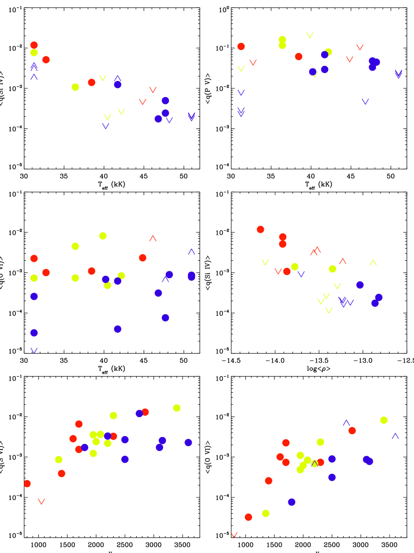
Figure 7: Mean ion fractions of different ions plotted as functions of the stellar parameters $T_{\rm eff}$, $\log\langle\rho\rangle$, and ${v}_{\infty}$. Different symbols represent either different values of $\log\langle\rho\rangle$ (for $\langle\rho\rangle$ in cgs units) or different temperatures. For plots with $T_{\rm eff}$ as the abscissa – red: $\log\langle\rho\rangle\leq-13.7$; yellow: $-13.7<\log\langle\rho\rangle\leq-13.2$; blue: $-13.2<\log\langle\rho\rangle$. For plots with $\log\langle\rho\rangle$ or ${v}_{\infty}$ as the abscissa – red: $T_{\rm eff}$ $\leq$ 38 kK; yellow: 38 $<$ $T_{\rm eff}$ $\leq$ 45 kK; blue: 45 kK $<$ $T_{\rm eff}$. Saturated points are indicated by upward-pointing arrowheads, while lower limits are shown as downward-pointing arrowheads.

Figure 7 shows selected mean ionization fractions, $\langle q_{i}\rangle$, listed in Table 8 plotted as functions of the adopted stellar parameters. In these plots, we employ the mean density of the wind, which we define as

$$\langle\rho\rangle\equiv\frac{\dot{M}}{4\pi v_{\infty}}\frac{\int_{0.2}^{0.9}r^{-2}v^{-1}dw}{\int_{0.2}^{0.9}dw}.$$ (8)

Whenever a plot has anything other than $T_{\rm eff}$ as the abscissa, the symbols are sorted by temperature according to the following scheme: red symbols for $T_{\rm eff}$ $\leq 38$kK yellow for $38<$ $T_{\rm eff}$ $\leq 45$kK and blue for $T_{\rm eff}$ $>45$kK. When $T_{\rm eff}$ is the abscissa, then the symbols are coded according to $\log\langle\rho\rangle$ (in cgs units) as follows: red for $\log\langle\rho\rangle\leq-13.7$, yellow for $-13.7<\log\langle\rho\rangle\leq-13.2$, and blue for $-13.2<\log\langle\rho\rangle$.

The first plot, $\langle q($Si iv$)\rangle$ versus $T_{\rm eff}$, shows a trend which is typical of ions with low ionization potentials – they tend to decrease in strength with increasing $T_{\rm eff}$, as expected. The plot $\langle q($P v$)\rangle$ versus $T_{\rm eff}$ shows that this trend vanishes for ions with ionization potentials equal to or greater than that of P v, implying that this may be a dominant ion. The next plot shows that $\langle q($O vi$)\rangle$ is also independent of $T_{\rm eff}$. Notice, however, that there is an indication that the level of $\langle q($O vi$)\rangle$ at a fixed $T_{\rm eff}$ may decrease with increasing wind density.

The $\langle q($Si iv$)\rangle$ versus $\log\langle\rho\rangle$ figure shows how plots containing limits can be deceiving. Although there is an apparent trend in the symbols, upper and lower limits are present at the same abscissa and over wide ranges. As a result, no strict relationship is present. At first, this might seem strange, since it is well known that the strength of Si iv is an excellent luminosity discriminant and that more luminous stars tend to have denser winds. However, a star with a large $\langle q_{i}\rangle$ for an ion need not have a strong wind line for that ion, since the observed line strength depends on $\dot{M}\langle q_{i}\rangle$.

Finally, the bottom panels of Figure 7 show the only ions which have a significant ${v}_{\infty}$ dependence. These are the super-ions, S vi and O vi (N v may as well, but it is difficult to be certain due to the large number of saturated points). Once again, S vi seems to be a “transition” species in the sense that the ion fractions of the cooler stars (red points) have a strong dependence on ${v}_{\infty}$, while there is effectively no correlation for the hottest stars (blue points). This relation between ion fraction and ${v}_{\infty}$ suggests a mechanical origin for these ions, since ${v}_{\infty}$ can be viewed as the potential for mechanical heating through shocks. Further, the fact that the ion fractions of S vi in the cooler stars and O vi in all stars do not depend on temperature or, equivalently, the radiation field of the underlying star, reinforces the idea that a non-radiative processes dominates their production.

6.5 Notes on Individual Stars

When placed in context, three stars stand out from the others.

BI 272. The wind lines of BI 272 indicate a much earlier spectral class than its uncertain classification of O7 II-III:. Its terminal velocity is quite large (3400 km s^-1), which suggests it is a dwarf. The only wind lines in its FUSE spectrum are O vi (quite strong), and S vi (clearly present, but fairly weak; see Table 7). It also has a strong, symmetric, C iii $\lambda$1176 feature. Its FOS spectrum has a strong N v $\lambda\lambda$1238, 1242 wind line, but its C iv $\lambda\lambda$1548,1550 line shows no sign of a wind all! Furthermore, the He ii $\lambda$1640 and N iv $\lambda$1718 lines in the FOS spectrum show no trace of a wind, again suggesting a star near the main sequence. Thus, the only wind lines in this star are from super-ions, and all the luminosity indicators in its spectrum point toward a near main sequence object. As a result, we suspect that either this star is extremely hot, or either its FUSE or FOS spectrum is composite. A high-quality optical spectrum would help distinguish between these possibilities.

BI 208. The wind profiles of BI 208 are very peculiar. Only the super-ions O vi and S vi exhibit P Cygni profiles in FUSE spectra, but the S vi lines are not especially useful because they are weak and compromised by interstellar absorption. Furthermore, the O vi profiles could not be fit self-consistently, and consequently are not listed in Table 7. The difficulties encountered with the SEI fits are illustrated in Figure 8. The upper panel shows a fit that reproduces the emission lobe reasonably well with a fast (${v}_{\infty}$$\sim$2500 km s^-1), optically thick outflow, but which produces too much absorption. Conversely, the lower panel shows that smaller values of $\tau_{rad}$ provide a good fit to the absorption trough, but fail to produce sufficient emission. Unfortunately, the archival FOS spectrum is suspect, primarily because its flux distribution slopes downward toward shorter wavelengths to a level that is significantly smaller than the flux in the FUSE spectrum at the same wavelength. However, if the wind profiles in the FOS spectrum can be trusted, they are also quite peculiar. For example, while N v $\lambda\lambda$1238, 1240 is strong and extends to about $-2000$ km s^-1 with substantial emission, the C iv $\lambda\lambda$1548, 1550 absorption is weak ($\sim$30% of the local continuum) and extends only to about $-1200$ km s^-1 with no discernible emission. The N v and C iv wind profiles of the rapidly rotating Galactic star HD 93521 exhibit similar morphologies, which Massa et al. (1995a) and Bjorkman et al. (1994) interpreted in terms of an outflow geometry that is cylindrically, not spherically, symmetric. The similarity extends to O vi, which is also characterized by strong emission for comparatively weak absorption in FUV spectra of HD 93521 obtained with the Tübingen Ultraviolet Echelle Spectrometer during the ORFEUS-SPAS mission in 1996 (Barnstedt et al., 2000). However, in order to make this morphological connection more convincingly, a reliable HST spectrum is required. It also would be of considerable interest to obtain high S/N optical spectra in order to determine whether BI 208 has a large $v\sin i$.

Sk $-67{{}^{\circ}}166$. The O4 supergiants Sk $-67{{}^{\circ}}166$ and Sk $-67{{}^{\circ}}167$ are neighbors in the young cluster NGC 2014. They are separated by $\sim$11.1′ on the sky, which corresponds to a projected distance of $\sim$163 pc for an adopted distance modulus of 18.52. Despite the similarity of their spectral types, Walborn et al. (1995; 1996; 2002a) noted that the relative strengths of the CNO wind lines are completely different, with C and O weaker and N much stronger in Sk $-67{{}^{\circ}}166$. Our quantitative analysis confirms this suspicion. The ratio of ion fractions in the sense Sk $-67{{}^{\circ}}166$ : Sk $-67{{}^{\circ}}167$ for the non-CNO ions Si iv, S iv, P v, and S vi are 0.76, 0.73, 0.84 and 0.64, respectively, with a mean of 0.74. Note that these ions bracket the full range of ionization, and effectively give the same result. In contrast, the three CNO lines that are unsaturated in at least one of the stars – C iii, N iii, and O vi – have ratios of 0.20, $\geq$1 and $\leq$0.10, respectively; i.e., the abundances of carbon and oxygen in Sk $-67{{}^{\circ}}166$ are several times less than in Sk $-67{{}^{\circ}}167$ and its nitrogen abundance is greater. This pattern of abundances is a signature of material processed through the CNO-cycle and implies that more processed material is present on the surface of Sk $-67{{}^{\circ}}166$ than Sk $-67{{}^{\circ}}167$; i.e., that Sk $-67{{}^{\circ}}166$ is an ON star. Unfortunately, the spectral properties of these stars do match closely enough to permit the more quantitative differential abundance analysis used by Massa et al. (1991). However, detailed modeling by Crowther et al. (2002) confirms that N is enhanced and C and O are depleted in the atmosphere Sk $-67{{}^{\circ}}166$ compared to normal LMC abundances.

7 Summary and Conclusions

Using the unique spectral coverage and sensitivity provided by FUSE and SEI modelling to translate the observed wind line profiles into quantitative information, we determined the following:

1. Because none of the derived ion fractions exceed unity, the mass loss rates determined by the Vink et al. (2000; 2001) formulae are not too small.

2. Because the P v ion fraction never approaches unity, as expected by models, we conclude that either

   1. the phosphorus abundance in the LMC is $\sim 1/3$ of the canonical value assumed for most elements, or

   2. the Vink et al. mass loss rates are 2 to 3 times too large, or

   3. some aspect of the models, such as their neglect of clumping in the winds, results in derived $\dot{M}q_{i}$ values that are $\sim 3$ times too small.

3. Ion ratios not involving N ions show much clearer $T_{\rm eff}$ dependence (with lower ions being more dominant in the cooler stars) than do ion ratios involving N ions. This result is attributed to a non-uniformity in the abundance of nitrogen, as a result of nuclear processing over the lifetimes of the stars.

4. Ion fractions of higher ions, that are not super-ions. decrease relative to lower ions as $w=v/$${v}_{\infty}$ increases.

5. Ionic ratios containing super-ions do not show a $w$ dependence. O vi exhibits this trait for all O stars, S vi shows it for only the coolest O stars, and the N v lines are too often saturated to distinguish between the early and late O stars. Together, this result implies that the production of O vi is non-radiative, and the same is true for S vi in the coolest O stars.

6. The mean ion fractions, $\langle q($S vi$)\rangle$ and $\langle q($O vi$)\rangle$, do not depend on the temperature of the star, again suggesting a non-radiative production mechanism,

7. The ion fractions of O vi in all stars and S vi in the later O stars are positively correlated with ${v}_{\infty}$, suggesting a shock strength dependence.

8. The wind lines in BI 272 are indicative of a considerably hotter star than is implied by its uncertain spectral.

9. BI 208 may have a non-spherical wind.

10. Sk $-67{{}^{\circ}}166$ is an ON star.

Figure 2: Examples of fits for S iv in Sk $-67{{}^{\circ}}111$ (left) and O vi in Sk $-70{{}^{\circ}}69$ (right). The velocity scales are in the stellar rest frames. The top panels show the raw model output, the observed spectrum, and the contributions to the model profile from transmitted and scattered light as functions of normalized velocity. A thick tick mark denotes the rest position of the red component of the doublet. The middle panels show $\tau_{rad}$ and the input photospheric profile as a function of normalized velocity. The bottom panels compare the observed profile to the model after application of an H i $+$ H₂ ISM model and convolution with the instrumental profile. See §3.3.

Figure 3: Observed wind profiles (solid curves) and fits (dotted curves) for selected program stars as a function of normalized velocity. The fits incorporate crude interstellar absorption models to demonstrate the impact of ISM absorption on the profiles. The name of the ion, star, and the rest position of the line or doublet are indicated in each panel.

Figure 4: Same as Figure 3

Figure 5: Comparison between between previous determinations of ${v}_{\infty}$ and the values derived in the present work. The dashed line indicates a one-to-one correlation, while the dotted lines denote offsets of $\pm$150 km s^-1 from this line.

Figure 8: Two attempts at fitting the O vi wind profile of BI 208. The solid curve is normalized stellar flux, while the dashed curve is the complete model with absorption from interstellar H i and H₂ included. Both wavelength scales are in the laboratory frame. The upper panel shows the best possible fit to the wind emission, and the bottom panel is the best fit to the wind absorption. Strong emission lines in the region of Ly $\beta$ are due to airglow.

Table 1: Fundamental Properties of Targets

Name	Alias	Spectral Type	Ref.	${v}_{\infty}$	$\log L_{\star}/\,{\rm L}_{\sun}$	$T_{\rm eff}$	$R_{\star}$	$\dot{M}$
				(km s-1)		(K)	(R☉)	($10^{-6}$ ${\rm M}_{\sun}/{\rm yr}$)
Sk $-67{{}^{\circ}}211$	HDE 269810	O2 III(f∗)	1	3600	6.32	50960	18.5	10.5 0
Sk $-66{{}^{\circ}}172$		O2 III(f∗)+OB	1	3100	6.12	50960	14.7	05.92
Sk $-70{{}^{\circ}}91$		O2 III(f∗)+OB	2	3150	6.12	50960	14.7	05.82
Sk $-67{{}^{\circ}}166$	HDE 269698	O4 If+	3	1800	6.26	47690	19.7	15.9 0
Sk $-67{{}^{\circ}}167$		O4 Inf+	4	2200	6.19	47690	18.2	10.1 0
Sk $-67{{}^{\circ}}69$		O4 III(f)	4	2500	6.02	48180	14.7	04.83
Sk $-71{{}^{\circ}}45$	HDE 269676	O4-5 III(f)	3	2500	6.58	46800	29.6	35.8 0
Sk $-70{{}^{\circ}}69$		O5 V	5	2750	5.49	46120	8.7	00.61
Sk $-70{{}^{\circ}}60$		O5-6 Vn((f))	6	2300	5.59	44840	10.3	01.03
Sk $-65{{}^{\circ}}22$	HDE 270952	O6 Iaf+	3	1350	6.22	41710	24.6	16.0 0
Sk $-67{{}^{\circ}}111$		O6 Ia(n)fp var	2	2000	6.01	41710	19.3	05.04
Sk $-66{{}^{\circ}}100$		O6 II(f)	5	2075	5.73	42170	13.7	01.78
Sk $-70{{}^{\circ}}115$	HDE 270145	O6.5 Iaf	6	2200	6.22	40210	26.5	09.46
BI 272		O7: III-II:	6	3400	5.65	39860	14.0	00.77
BI 229		O7 V-III	6	1950	5.86	40440	17.3	02.91
BI 208		O7 Vn	6	$\cdots$	5.38	41010	9.7	$\cdots$
Sk $-67{{}^{\circ}}101$		O8 II((f))	2	2300	5.83	36410	20.6	01.99
BI 173		O8 II:	2	2850	5.72	36410	18.2	01.08
Sk $-67{{}^{\circ}}191$		O8 V	7	1950	5.53	38450	13.1	00.83
Sk $-69{{}^{\circ}}124$		O9 Ib	7	1600	5.60	32740	19.6	01.12
BI 170		O9.5 Ib	2	1700	5.43	31240	17.7	00.54
Sk $-66{{}^{\circ}}169$		O9.7 Ia+	8	0800	6.09	31240	37.8	12.6 0
Sk $-68{{}^{\circ}}135$	HDE 269896	ON9.7 Ia+	3	1050	6.33	31240	49.8	23.0 0
Sk $-65{{}^{\circ}}21$		O9.7 Iab	5	1700	5.87	31240	29.4	02.67
Sk $-67{{}^{\circ}}05$	HDE 268605	O9.7 Ib	3	1400	6.19	31240	42.4	10.4 0

Table 2: Sources of Photometric and Spectroscopic Data

Name	$V$	(B V)	Ref.	$E$(B V)	$F_{\lambda}$(1150 Å)	FUSE	HST/FOS, HST/STIS, IUE
Sk $-67{{}^{\circ}}211$	12.28	$-$0.23	1	0.09	33.7	P1171603	FOS: Y14M0D05T
Sk $-66{{}^{\circ}}172$	13.13	$-$0.12	2	0.20	10.7	P1172201	FOS: Y0YG0903T, 4T, 5T
Sk $-70{{}^{\circ}}91$	12.78	$-$0.23	3	0.09	17.0	P1172501	FOS: Y25U0L01T
Sk $-67{{}^{\circ}}166$	12.27	$-$0.22	1	0.10	28.4	A1330101 – 62	IUE: SWP 6967
Sk $-67{{}^{\circ}}167$	12.54	$-$0.19	4	0.13	21.9	P1171901, 2	FOS: Y14M0C09T
Sk $-67{{}^{\circ}}69$	13.09	$-$0.16	3	0.16	10.4	P1171703	$\cdots$
Sk $-71{{}^{\circ}}45$	11.51	$-$0.19	5	0.13	26.3	P1031501 – 4	STIS: O63521010
Sk $-70{{}^{\circ}}69$	13.94	$-$0.27:	2	0.05	10.4	P1171703	FOS: Y0YG0703T, 4T, 5T, 6T
Sk $-70{{}^{\circ}}60$	13.85	$-$0.19	2	0.13	05.8	P1172001	FOS: Y25U0I01T
Sk $-65{{}^{\circ}}22$	12.07	$-$0.19	3	0.13	31.3	P1031002	FOS: Y25U1401T
Sk $-67{{}^{\circ}}111$	12.57	$-$0.20	4	0.12	18.0	P1173001	IUE: SWP 10991
Sk $-66{{}^{\circ}}100$	13.26	$-$0.21	3	0.11	11.7	P1172303	FOS: Y0YG0803T, 4T
Sk $-70{{}^{\circ}}115$	12.24	$-$0.10	4	0.22	20.3	P1172601	$\cdots$
BI 272	13.28	$-$0.22	6	0.10	10.9	P1172901, 2	FOS: Y25U1001T
BI 229	12.95	$-$0.17	7	0.15	20.8	P1172801	FOS: Y25U0U01T
BI 208	13.96	$-$0.24	6	0.07	05.9	P1172702 – 5	FOS: Y25U0M01T
Sk $-67{{}^{\circ}}101$	12.63	$-$0.17	4	0.13	17.7	P1173401, 3	STIS: O4YN01020
BI 173	13.00	$-$0.14	7	0.16	07.5	P1173201, 2	FOS: Y25U0W01T
Sk $-67{{}^{\circ}}191$	13.46	$-$0.21	3	0.10	08.2	P1173101, 2	FOS: Y25U0O01T
Sk $-69{{}^{\circ}}124$	12.81	$-$0.18	6	0.10	09.0	P1173601, 2	FOS: Y25U1601T
BI 170	13.09	$-$0.17	7	0.10	09.0	P1173701	FOS: Y25U1201T
Sk $-66{{}^{\circ}}169$	11.56	$-$0.13	8	0.14	26.3	P1173801	IUE: SWP 47601
Sk $-68{{}^{\circ}}135$	11.36	0.00	1	0.27	06.5	P1173901	IUE: SWP 47594, 55216
Sk $-65{{}^{\circ}}21$	12.02	$-$0.16	4	0.11	16.5	P1030901 – 3	IUE: SWP 16604, 17891
Sk $-67{{}^{\circ}}05$	11.34	$-$0.12	1	0.15	25.0	P1030703, 4	IUE: SWP 51851, 52010

Table 3: Properties of FUV and UV Resonance Lines

Ion	Abundance	I.P. Range	$\lambda_{\rm blue}$	$\lambda_{\rm red}$	$\Delta v$	$f_{\rm blue}$	$f_{\rm red}$
		(eV)	(Å)	(Å)	(km s-1)
C iii	8.55	24.383 – 47.887	977.020	$\cdots$	$\cdots$	0.759	$\cdots$
C iv	8.55	47.887 – 64.492	1548.203	1550.777	0498	0.191	0.0952
N iii	7.97	29.601 – 47.448	989.799	991.571	0537	0.123	0.122
N v	7.97	77.472 – 97.888	1238.821	1252.804	0964	0.156	0.078
O vi	8.87	113.896 – 138.116	1031.926	1037.617	1653	0.133	0.0659
Si iv	7.55	33.492 – 45.141	1393.755	1402.770	1939	0.5140	0.2553
P iv	5.57	30.18 – 51.37	950.657	$\cdots$	$\cdots$	1.560	$\cdots$
P v	5.57	051.37 – 65.023	1117.977	1128.008	2690	0.473	0.234
S iv	7.27	34.83 – 47.30	1062.664	1073.028	2924	0.0400	0.0397
S vi	7.27	072.68 – 88.049	933.378	944.523	3580	0.439	0.217

Table 4: Parameters of Photospheric Features

Name	S vi	N v	C iv	P v	S iv	Si iv	C iii	N iii
Sk $-67{{}^{\circ}}211$	3.0 , 200	0.0 ,000	8.1 , 300	$\cdots$	$\cdots$	$\cdots$	$\cdots$	$\cdots$
Sk $-66{{}^{\circ}}172$	0.0 ,000	2.0 , 250	2.0 , 250	$\cdots$	$\cdots$	$\cdots$	$\cdots$	$\cdots$
Sk $-70{{}^{\circ}}91$	0.0 ,000	0.0 ,000	4.0 , 250	$\cdots$	$\cdots$	$\cdots$	$\cdots$	$\cdots$
Sk $-67{{}^{\circ}}166$	3.0 , 200	1.5 , 149	1.0 , 101	2.0 , 200	0.0 ,000	3.0 , 300	2.0 , 200	6.0 , 200
Sk $-67{{}^{\circ}}167$	5.0 , 200	0.0 ,000	1.0 , 101	2.0 , 300	0.5 , 98	1.0 , 400	0.2 , 101	2.0 , 150
Sk $-67{{}^{\circ}}69$	2.0 , 300	$\cdots$	$\cdots$	2.0 , 300	$\cdots$	$\cdots$	2.0 , 300	2.0 , 300
Sk $-71{{}^{\circ}}45$	0.0 ,000	2.0 , 250	0.0 ,000	$\cdots$	$\cdots$	2.0 , 250	$\cdots$	$\cdots$
Sk $-70{{}^{\circ}}69$	5.0 , 200	3.0 , 200	1.0 , 200	$\cdots$	$\cdots$	$\cdots$	$\cdots$	$\cdots$
Sk $-70{{}^{\circ}}60$	0.0 ,000	0.0 ,000	2.0 , 200	$\cdots$	$\cdots$	$\cdots$	$\cdots$	$\cdots$
Sk $-65{{}^{\circ}}22$	0.0 ,000	0.0 ,000	4.0 , 200	2.0 , 200	2.0 , 201	4.0 , 200	4.0 , 200	2.0 , 250
Sk $-67{{}^{\circ}}111$	5.0 , 300	4.0 , 200	5.1 , 200	2.0 , 250	1.0 , 400	3.0 , 200	5.0 , 300	1.0 , 300
Sk $-66{{}^{\circ}}100$	0.0 ,000	5.0 , 200	3.0 , 200	5.0 , 250	$\cdots$	$\cdots$	5.0 , 250	5.0 , 250
Sk $-70{{}^{\circ}}115$	0.0 ,000	$\cdots$	$\cdots$	5.0 , 200	$\cdots$	$\cdots$	3.0 , 200	3.0 , 200
BI 272	0.0 ,000	0.0 ,000	$\cdots$	$\cdots$	$\cdots$	$\cdots$	$\cdots$	$\cdots$
BI 229	3.0 , 200	2.0 , 200	3.0 , 200	$\cdots$	$\cdots$	$\cdots$	$\cdots$	$\cdots$
Sk $-67{{}^{\circ}}101$	3.0 , 300	0.0 ,000	4.0 , 300	5.0 , 300	$\cdots$	5.0 , 300	5.0 , 300	5.0 , 300
BI 173	2.0 , 300	0.0 ,000	0.0 ,000	3.0 , 300	$\cdots$	$\cdots$	5.0 , 300	5.0 , 300
Sk $-67{{}^{\circ}}191$	0.0 ,000	2.0 , 400	5.1 , 200	3.0 , 300	$\cdots$	2.0 , 400	$\cdots$	3.0 , 300
Sk $-69{{}^{\circ}}124$	0.0 ,000	$\cdots$	5.0 , 300	$\cdots$	5.1 , 300	5.0 , 300	5.0 , 300	5.0 , 300
BI 170	0.0 ,000	0.0 ,000	5.0 , 300	5.0 , 300	5.1 , 300	3.0 , 300	5.0 , 300	5.0 , 300
Sk $-66{{}^{\circ}}169$	2.0 , 300	0.0 ,000	5.0 , 300	$\cdots$	5.1 , 300	5.0 , 300	$\cdots$	$\cdots$
Sk $-68{{}^{\circ}}135$	$\cdots$	0.0 ,000	5.0 , 300	$\cdots$	5.1 , 300	5.0 , 300	$\cdots$	$\cdots$
Sk $-65{{}^{\circ}}21$	0.0 ,000	0.0 ,000	4.0 , 300	$\cdots$	4.1 , 300	4.0 , 300	4.0 , 300	4.0 , 300
Sk $-67{{}^{\circ}}05$	0.0 ,000	0.0 ,000	5.0 , 300	$\cdots$	5.1 , 300	5.0 , 300	5.0 , 300	5.0 , 300

Note. — The entries give the adopted values of $(\tau_{0}^{B},v_{G})$, with $v_{G}$ in km s^-1. Zeros indicate a flat continuum; ellipsis indicate that the line was not fit. Flat continua were adopted for the O vi lines, with two exceptions: (a) for Sk $-67{{}^{\circ}}167$ we used $(\tau_{0}^{B},v_{G})=(4.9,~{}200)$; and (b) for Sk $-66{{}^{\circ}}169$ the O vi wind lines were not fit.

Table 5: Measured Parameters of the Wind Velocity Law

Name	${v}_{\infty}$	$\beta$					$w_{D}$
	(km s-1)		O vi	S vi	N v	C iv	P v	S iv	Si iv	C iii	N iii
Sk $-67{{}^{\circ}}211$	3600	0.8	0.06	0.06	0.06	0.06	$\cdots$	$\cdots$	$\cdots$	$\cdots$	$\cdots$
Sk $-66{{}^{\circ}}172$	3100	1.0	0.08	0.08	0.10	0.08	$\cdots$	$\cdots$	$\cdots$	$\cdots$	$\cdots$
Sk $-70{{}^{\circ}}91$	3150	1.0	0.05	0.06	0.10	0.06	$\cdots$	$\cdots$	$\cdots$	$\cdots$	$\cdots$
Sk $-67{{}^{\circ}}166$	1800	1.0	0.15	0.15	0.15	0.15	0.15	0.15	0.15	0.15	0.15
Sk $-67{{}^{\circ}}167$	2200	1.0	0.15	0.15	0.20	0.15	0.10	0.10	0.10	0.10	0.10
Sk $-67{{}^{\circ}}69$	2500	1.0	0.08	0.08	$\cdots$	$\cdots$	0.08	$\cdots$	$\cdots$	0.08	0.08
Sk $-71{{}^{\circ}}45$	2500	0.8	0.08	0.08	0.08	0.08	$\cdots$	$\cdots$	0.08	$\cdots$	$\cdots$
Sk $-70{{}^{\circ}}69$	2750	1.0	0.05	0.05	0.10	0.10	$\cdots$	$\cdots$	$\cdots$	$\cdots$	$\cdots$
Sk $-70{{}^{\circ}}60$	2300	0.5	0.04	0.05	0.07	0.10	$\cdots$	$\cdots$	$\cdots$	$\cdots$	$\cdots$
Sk $-65{{}^{\circ}}22$	1350	1.0	0.16	0.15	0.15	0.10	0.10	0.15	0.10	0.12	0.15
Sk $-67{{}^{\circ}}111$	2000	1.0	0.10	0.10	0.10	0.10	0.10	0.03	0.10	0.10	0.10
Sk $-66{{}^{\circ}}100$	2075	0.8	0.08	0.07	0.10	0.10	0.10	$\cdots$	$\cdots$	0.07	0.07
Sk $-70{{}^{\circ}}115$	2200	1.0	0.06	0.04	$\cdots$	$\cdots$	0.06	$\cdots$	$\cdots$	0.06	0.06
BI 272	3400	1.0	0.05	0.05	0.05	$\cdots$	$\cdots$	$\cdots$	$\cdots$	$\cdots$	$\cdots$
BI 229	1950	1.0	0.05	0.10	0.10	0.05	$\cdots$	$\cdots$	$\cdots$	$\cdots$	$\cdots$
Sk $-67{{}^{\circ}}101$	2300	1.0	0.10	0.10	0.10	0.10	0.10	$\cdots$	0.10	0.10	0.10
BI 173	2850	0.7	0.10	0.10	0.10	0.10	0.10	$\cdots$	$\cdots$	0.10	0.10
Sk $-67{{}^{\circ}}191$	1950	1.0	0.10	0.10	0.10	0.10	0.10	$\cdots$	0.10	$\cdots$	0.10
Sk $-69{{}^{\circ}}124$	1600	1.0	0.20	0.15	$\cdots$	0.30	$\cdots$	0.20	0.30	0.20	0.20
BI 170	1700	1.0	0.10	0.10	0.15	0.15	0.10	0.10	0.15	0.10	0.10
Sk $-66{{}^{\circ}}169$	0800	2.0	$\cdots$	0.10	0.20	0.10	$\cdots$	0.10	0.20	$\cdots$	$\cdots$
Sk $-68{{}^{\circ}}135$	1050	1.0	0.02	$\cdots$	0.05	0.03	$\cdots$	0.07	0.03	$\cdots$	$\cdots$
Sk $-65{{}^{\circ}}21$	1700	1.0	0.10	0.10	0.10	0.10	$\cdots$	0.10	0.10	0.10	0.10
Sk $-67{{}^{\circ}}05$	1400	1.0	0.05	0.05	0.05	0.05	$\cdots$	0.05	0.05	0.05	0.05

Table 6: Comparison with Previous Determinations of the Velocity Law

Name	Present Work	Haser	PP	PC	Other
	${v}_{\infty}$, $\beta$	${v}_{\infty}$, $\beta$	${v}_{\infty}$, $\beta$	${v}_{\infty}$	${v}_{\infty}$
Sk $-67{{}^{\circ}}211$	3600, 0.8	3750, 0.55	$\cdots$	$\cdots$	3800
Sk $-66{{}^{\circ}}172$	3100, 1.0	3250, 0.70	$\cdots$	2950	$\cdots$
Sk $-67{{}^{\circ}}166$	1800, 1.0	1900, 0.70	2250, 1.1	1735	2020
Sk $-67{{}^{\circ}}167$	2200, 1.0	2150, 0.70	$\cdots$	2005	$\cdots$
Sk $-70{{}^{\circ}}69$	2750, 1.0	2600, 1.00	$\cdots$	$\cdots$	$\cdots$
Sk $-70{{}^{\circ}}60$	2300, 1.0	$\cdots$	$\cdots$	2150	$\cdots$
Sk $-67{{}^{\circ}}111$	2000, 1.0	$\cdots$	2090, 0.7	$\cdots$	1800
Sk $-66{{}^{\circ}}100$	2075, 1.0	2150, 0.70	$\cdots$	1975	$\cdots$
BI 229	1950, 1.0	$\cdots$	$\cdots$	1980	$\cdots$
Sk $-67{{}^{\circ}}101$	2300, 1.0	$\cdots$	$\cdots$	2005	$\cdots$
Sk $-67{{}^{\circ}}191$	1950, 1.0	$\cdots$	$\cdots$	1750	$\cdots$
Sk $-69{{}^{\circ}}124$	1600, 1.0	$\cdots$	$\cdots$	1430	$\cdots$
BI 170	1700, 1.0	$\cdots$	$\cdots$	1370	$\cdots$
Sk $-65{{}^{\circ}}21$	1700, 1.0	1700, 1.00	$\cdots$	1330	$\cdots$
Sk $-67{{}^{\circ}}05$	1400, 1.0	$\cdots$	1665, 0.7	$\cdots$	$\cdots$

Note. — All values of ${v}_{\infty}$ are in km s^-1.

Table 7: Measured Ion Fractions

$v/v_{\infty}$	C iii	N iii	Si iv	S iv	C iv	P v	N v	S vi	O vi
Sk $-67{{}^{\circ}}211$
0.01	$\cdots$	$\cdots$	$\cdots$	$\cdots$	$2.1~{}(-5)$	$\cdots$	$>7~{}(-3)$	$1.4~{}(-3)$	$>4~{}(-4)$
0.05	$\cdots$	$\cdots$	$\cdots$	$\cdots$	$4.2~{}(-5)$	$\cdots$	$>1~{}(-2)$	$2.9~{}(-3)$	$>8~{}(-4)$
0.10	$\cdots$	$\cdots$	$\cdots$	$\cdots$	$6.8~{}(-5)$	$\cdots$	$>2~{}(-2)$	$4.7~{}(-3)$	$>1~{}(-3)$
0.15	$\cdots$	$\cdots$	$\cdots$	$\cdots$	$9.1~{}(-5)$	$\cdots$	$>3~{}(-2)$	$5.1~{}(-3)$	$>1~{}(-3)$
0.20	$\cdots$	$\cdots$	$\cdots$	$\cdots$	$1.1~{}(-4)$	$\cdots$	$>4~{}(-2)$	$4.7~{}(-3)$	$>2~{}(-3)$
0.25	$\cdots$	$\cdots$	$\cdots$	$\cdots$	$1.7~{}(-4)$	$\cdots$	$>5~{}(-2)$	$3.7~{}(-3)$	$>2~{}(-3)$
0.30	$\cdots$	$\cdots$	$\cdots$	$\cdots$	$1.9~{}(-4)$	$\cdots$	$>5~{}(-2)$	$3.2~{}(-3)$	$>3~{}(-3)$
0.35	$\cdots$	$\cdots$	$\cdots$	$\cdots$	$2.1~{}(-4)$	$\cdots$	$>6~{}(-2)$	$2.4~{}(-3)$	$>3~{}(-3)$
0.40	$\cdots$	$\cdots$	$\cdots$	$\cdots$	$2.8~{}(-4)$	$\cdots$	$>7~{}(-2)$	$1.8~{}(-3)$	$>3~{}(-3)$
0.45	$\cdots$	$\cdots$	$\cdots$	$\cdots$	$3.1~{}(-4)$	$\cdots$	$>7~{}(-2)$	$2.0~{}(-3)$	$>4~{}(-3)$
0.50	$\cdots$	$\cdots$	$\cdots$	$\cdots$	$3.3~{}(-4)$	$\cdots$	$>8~{}(-2)$	$1.5~{}(-3)$	$>4~{}(-3)$
0.55	$\cdots$	$\cdots$	$\cdots$	$\cdots$	$4.5~{}(-4)$	$\cdots$	$>2~{}(-2)$	$1.7~{}(-3)$	$>4~{}(-3)$
0.60	$\cdots$	$\cdots$	$\cdots$	$\cdots$	$4.8~{}(-4)$	$\cdots$	$>2~{}(-2)$	$1.4~{}(-3)$	$>5~{}(-3)$
0.65	$\cdots$	$\cdots$	$\cdots$	$\cdots$	$5.7~{}(-4)$	$\cdots$	$>3~{}(-2)$	$1.5~{}(-3)$	$>5~{}(-3)$
0.70	$\cdots$	$\cdots$	$\cdots$	$\cdots$	$6.1~{}(-4)$	$\cdots$	$>2~{}(-2)$	$1.2~{}(-3)$	$>5~{}(-3)$
0.75	$\cdots$	$\cdots$	$\cdots$	$\cdots$	$6.4~{}(-4)$	$\cdots$	$>1~{}(-2)$	$1.2~{}(-3)$	$>5~{}(-3)$
0.80	$\cdots$	$\cdots$	$\cdots$	$\cdots$	$6.7~{}(-4)$	$\cdots$	$6.0~{}(-3)$	$1.3~{}(-3)$	$>4~{}(-3)$
0.85	$\cdots$	$\cdots$	$\cdots$	$\cdots$	$7.0~{}(-4)$	$\cdots$	$6.2~{}(-3)$	$9.1~{}(-4)$	$>3~{}(-3)$
0.90	$\cdots$	$\cdots$	$\cdots$	$\cdots$	$7.3~{}(-4)$	$\cdots$	$5.2~{}(-3)$	$9.5~{}(-4)$	$1.8~{}(-3)$
0.95	$\cdots$	$\cdots$	$\cdots$	$\cdots$	$7.6~{}(-4)$	$\cdots$	$5.4~{}(-3)$	$5.0~{}(-4)$	$9.5~{}(-4)$
1.00	$\cdots$	$\cdots$	$\cdots$	$\cdots$	$7.9~{}(-4)$	$\cdots$	$5.6~{}(-3)$	$5.2~{}(-4)$	$9.8~{}(-4)$
Sk $-66{{}^{\circ}}172$
0.01	$\cdots$	$\cdots$	$\cdots$	$\cdots$	$3.7~{}(-6)$	$\cdots$	$>6~{}(-4)$	$1.4~{}(-4)$	$>4~{}(-5)$
0.05	$\cdots$	$\cdots$	$\cdots$	$\cdots$	$1.8~{}(-5)$	$\cdots$	$>3~{}(-3)$	$6.8~{}(-4)$	$>2~{}(-4)$
0.10	$\cdots$	$\cdots$	$\cdots$	$\cdots$	$3.7~{}(-5)$	$\cdots$	$>5~{}(-3)$	$1.4~{}(-3)$	$>4~{}(-4)$
0.15	$\cdots$	$\cdots$	$\cdots$	$\cdots$	$5.5~{}(-5)$	$\cdots$	$>8~{}(-3)$	$2.0~{}(-3)$	$>6~{}(-4)$
0.20	$\cdots$	$\cdots$	$\cdots$	$\cdots$	$7.3~{}(-5)$	$\cdots$	$>1~{}(-2)$	$2.7~{}(-3)$	$>9~{}(-4)$
0.25	$\cdots$	$\cdots$	$\cdots$	$\cdots$	$1.1~{}(-4)$	$\cdots$	$>1~{}(-2)$	$1.7~{}(-3)$	$>1~{}(-3)$
0.30	$\cdots$	$\cdots$	$\cdots$	$\cdots$	$1.3~{}(-4)$	$\cdots$	$>1~{}(-2)$	$2.0~{}(-3)$	$1.2~{}(-3)$
0.35	$\cdots$	$\cdots$	$\cdots$	$\cdots$	$1.5~{}(-4)$	$\cdots$	$>1~{}(-2)$	$1.9~{}(-3)$	$1.4~{}(-3)$
0.40	$\cdots$	$\cdots$	$\cdots$	$\cdots$	$1.7~{}(-4)$	$\cdots$	$>1~{}(-2)$	$2.2~{}(-3)$	$1.0~{}(-3)$
0.45	$\cdots$	$\cdots$	$\cdots$	$\cdots$	$1.9~{}(-4)$	$\cdots$	$>1~{}(-2)$	$1.5~{}(-3)$	$1.2~{}(-3)$
0.50	$\cdots$	$\cdots$	$\cdots$	$\cdots$	$2.4~{}(-4)$	$\cdots$	$>1~{}(-2)$	$1.7~{}(-3)$	$6.4~{}(-4)$
0.55	$\cdots$	$\cdots$	$\cdots$	$\cdots$	$2.7~{}(-4)$	$\cdots$	$>1~{}(-2)$	$1.9~{}(-3)$	$7.1~{}(-4)$
0.60	$\cdots$	$\cdots$	$\cdots$	$\cdots$	$2.9~{}(-4)$	$\cdots$	$>1~{}(-2)$	$2.0~{}(-3)$	$7.7~{}(-4)$
0.65	$\cdots$	$\cdots$	$\cdots$	$\cdots$	$4.0~{}(-4)$	$\cdots$	$>1~{}(-2)$	$2.2~{}(-3)$	$8.4~{}(-4)$
0.70	$\cdots$	$\cdots$	$\cdots$	$\cdots$	$4.3~{}(-4)$	$\cdots$	$>1~{}(-2)$	$2.4~{}(-3)$	$9.0~{}(-4)$
0.75	$\cdots$	$\cdots$	$\cdots$	$\cdots$	$4.6~{}(-4)$	$\cdots$	$>1~{}(-2)$	$1.0~{}(-3)$	$5.8~{}(-4)$
0.80	$\cdots$	$\cdots$	$\cdots$	$\cdots$	$7.3~{}(-4)$	$\cdots$	$5.9~{}(-3)$	$1.1~{}(-3)$	$6.2~{}(-4)$
0.85	$\cdots$	$\cdots$	$\cdots$	$\cdots$	$1.0~{}(-3)$	$\cdots$	$6.3~{}(-3)$	$1.2~{}(-3)$	$6.6~{}(-4)$
0.90	$\cdots$	$\cdots$	$\cdots$	$\cdots$	$1.1~{}(-3)$	$\cdots$	$9.9~{}(-3)$	$6.1~{}(-4)$	$5.8~{}(-4)$
0.95	$\cdots$	$\cdots$	$\cdots$	$\cdots$	$1.3~{}(-3)$	$\cdots$	$1.0~{}(-2)$	$6.4~{}(-4)$	$8.3~{}(-4)$
1.00	$\cdots$	$\cdots$	$\cdots$	$\cdots$	$1.5~{}(-3)$	$\cdots$	$>1~{}(-2)$	$6.8~{}(-4)$	$2.6~{}(-3)$
Sk $-70{{}^{\circ}}91$
0.01	$\cdots$	$\cdots$	$\cdots$	$\cdots$	$5.1~{}(-6)$	$\cdots$	$>4~{}(-4)$	$4.3~{}(-4)$	$>6~{}(-5)$
0.05	$\cdots$	$\cdots$	$\cdots$	$\cdots$	$2.6~{}(-5)$	$\cdots$	$>2~{}(-3)$	$1.8~{}(-3)$	$>2~{}(-4)$
0.10	$\cdots$	$\cdots$	$\cdots$	$\cdots$	$5.1~{}(-5)$	$\cdots$	$>3~{}(-3)$	$2.8~{}(-3)$	$>4~{}(-4)$
0.15	$\cdots$	$\cdots$	$\cdots$	$\cdots$	$7.7~{}(-5)$	$\cdots$	$>4~{}(-3)$	$3.2~{}(-3)$	$6.1~{}(-4)$
0.20	$\cdots$	$\cdots$	$\cdots$	$\cdots$	$1.0~{}(-4)$	$\cdots$	$>3~{}(-3)$	$3.1~{}(-3)$	$7.0~{}(-4)$
0.25	$\cdots$	$\cdots$	$\cdots$	$\cdots$	$1.3~{}(-4)$	$\cdots$	$>3~{}(-3)$	$2.8~{}(-3)$	$7.8~{}(-4)$
0.30	$\cdots$	$\cdots$	$\cdots$	$\cdots$	$1.5~{}(-4)$	$\cdots$	$3.5~{}(-3)$	$2.6~{}(-3)$	$8.1~{}(-4)$
0.35	$\cdots$	$\cdots$	$\cdots$	$\cdots$	$1.8~{}(-4)$	$\cdots$	$2.7~{}(-3)$	$2.5~{}(-3)$	$8.0~{}(-4)$
0.40	$\cdots$	$\cdots$	$\cdots$	$\cdots$	$1.9~{}(-4)$	$\cdots$	$2.3~{}(-3)$	$2.6~{}(-3)$	$8.1~{}(-4)$
0.45	$\cdots$	$\cdots$	$\cdots$	$\cdots$	$2.2~{}(-4)$	$\cdots$	$1.7~{}(-3)$	$2.6~{}(-3)$	$8.5~{}(-4)$
0.50	$\cdots$	$\cdots$	$\cdots$	$\cdots$	$2.4~{}(-4)$	$\cdots$	$1.7~{}(-3)$	$2.5~{}(-3)$	$8.1~{}(-4)$
0.55	$\cdots$	$\cdots$	$\cdots$	$\cdots$	$2.6~{}(-4)$	$\cdots$	$1.7~{}(-3)$	$2.7~{}(-3)$	$8.9~{}(-4)$
0.60	$\cdots$	$\cdots$	$\cdots$	$\cdots$	$2.7~{}(-4)$	$\cdots$	$1.9~{}(-3)$	$2.6~{}(-3)$	$8.1~{}(-4)$
0.65	$\cdots$	$\cdots$	$\cdots$	$\cdots$	$2.9~{}(-4)$	$\cdots$	$2.3~{}(-3)$	$2.8~{}(-3)$	$8.8~{}(-4)$
0.70	$\cdots$	$\cdots$	$\cdots$	$\cdots$	$3.1~{}(-4)$	$\cdots$	$2.7~{}(-3)$	$2.5~{}(-3)$	$8.5~{}(-4)$
0.75	$\cdots$	$\cdots$	$\cdots$	$\cdots$	$3.4~{}(-4)$	$\cdots$	$2.9~{}(-3)$	$2.1~{}(-3)$	$7.6~{}(-4)$
0.80	$\cdots$	$\cdots$	$\cdots$	$\cdots$	$3.6~{}(-4)$	$\cdots$	$3.7~{}(-3)$	$2.3~{}(-3)$	$8.1~{}(-4)$
0.85	$\cdots$	$\cdots$	$\cdots$	$\cdots$	$3.8~{}(-4)$	$\cdots$	$3.9~{}(-3)$	$1.8~{}(-3)$	$6.9~{}(-4)$
0.90	$\cdots$	$\cdots$	$\cdots$	$\cdots$	$4.6~{}(-4)$	$\cdots$	$4.2~{}(-3)$	$1.9~{}(-3)$	$6.7~{}(-4)$
0.95	$\cdots$	$\cdots$	$\cdots$	$\cdots$	$6.1~{}(-4)$	$\cdots$	$4.4~{}(-3)$	$2.0~{}(-3)$	$6.4~{}(-4)$
1.00	$\cdots$	$\cdots$	$\cdots$	$\cdots$	$6.4~{}(-4)$	$\cdots$	$4.6~{}(-3)$	$2.1~{}(-3)$	$6.7~{}(-4)$
Sk $-67{{}^{\circ}}166$
0.01	$8.1~{}(-8)$	$5.7~{}(-6)$	$2.8~{}(-6)$	$1.1~{}(-5)$	$>6~{}(-6)$	$1.7~{}(-3)$	$>6~{}(-5)$	$6.3~{}(-5)$	$3.8~{}(-6)$
0.05	$4.1~{}(-7)$	$2.9~{}(-5)$	$1.4~{}(-5)$	$5.5~{}(-5)$	$>3~{}(-5)$	$8.4~{}(-3)$	$>3~{}(-4)$	$3.1~{}(-4)$	$1.9~{}(-5)$
0.10	$8.2~{}(-7)$	$5.7~{}(-5)$	$2.8~{}(-5)$	$1.1~{}(-4)$	$>6~{}(-5)$	$1.7~{}(-2)$	$>6~{}(-4)$	$6.3~{}(-4)$	$2.7~{}(-5)$
0.15	$1.2~{}(-6)$	$8.6~{}(-5)$	$4.2~{}(-5)$	$1.7~{}(-4)$	$>9~{}(-5)$	$1.5~{}(-2)$	$>9~{}(-4)$	$9.4~{}(-4)$	$4.1~{}(-5)$
0.20	$1.6~{}(-6)$	$1.1~{}(-4)$	$5.5~{}(-5)$	$2.2~{}(-4)$	$>1~{}(-4)$	$2.0~{}(-2)$	$>1~{}(-3)$	$1.3~{}(-3)$	$4.3~{}(-5)$
0.25	$2.0~{}(-6)$	$2.9~{}(-4)$	$6.9~{}(-5)$	$2.8~{}(-4)$	$>1~{}(-4)$	$2.1~{}(-2)$	$>1~{}(-3)$	$1.4~{}(-3)$	$5.4~{}(-5)$
0.30	$2.4~{}(-6)$	$3.4~{}(-4)$	$8.3~{}(-5)$	$3.3~{}(-4)$	$>1~{}(-4)$	$2.5~{}(-2)$	$>1~{}(-3)$	$1.7~{}(-3)$	$4.9~{}(-5)$
0.35	$2.9~{}(-6)$	$8.0~{}(-4)$	$9.7~{}(-5)$	$3.9~{}(-4)$	$>2~{}(-4)$	$2.4~{}(-2)$	$>2~{}(-3)$	$2.0~{}(-3)$	$5.7~{}(-5)$
0.40	$3.3~{}(-6)$	$1.4~{}(-3)$	$1.1~{}(-4)$	$6.7~{}(-4)$	$>2~{}(-4)$	$2.7~{}(-2)$	$>2~{}(-3)$	$2.3~{}(-3)$	$5.2~{}(-5)$
0.45	$5.5~{}(-6)$	$>2~{}(-3)$	$1.4~{}(-4)$	$7.5~{}(-4)$	$>2~{}(-4)$	$3.0~{}(-2)$	$>2~{}(-3)$	$2.1~{}(-3)$	$5.9~{}(-5)$
0.50	$8.2~{}(-6)$	$>2~{}(-3)$	$1.6~{}(-4)$	$1.4~{}(-3)$	$>3~{}(-4)$	$3.4~{}(-2)$	$>3~{}(-3)$	$2.3~{}(-3)$	$6.5~{}(-5)$
0.55	$1.1~{}(-5)$	$>2~{}(-3)$	$2.2~{}(-4)$	$1.5~{}(-3)$	$>3~{}(-4)$	$3.7~{}(-2)$	$>3~{}(-3)$	$2.2~{}(-3)$	$7.2~{}(-5)$
0.60	$1.5~{}(-5)$	$>3~{}(-3)$	$2.4~{}(-4)$	$3.3~{}(-3)$	$>3~{}(-4)$	$4.1~{}(-2)$	$>3~{}(-3)$	$2.4~{}(-3)$	$7.8~{}(-5)$
0.65	$2.1~{}(-5)$	$>3~{}(-3)$	$3.1~{}(-4)$	$3.6~{}(-3)$	$>4~{}(-4)$	$4.4~{}(-2)$	$>4~{}(-3)$	$1.9~{}(-3)$	$9.9~{}(-5)$
0.70	$3.7~{}(-5)$	$>4~{}(-3)$	$3.3~{}(-4)$	$3.9~{}(-3)$	$>4~{}(-4)$	$4.7~{}(-2)$	$>4~{}(-3)$	$2.0~{}(-3)$	$1.1~{}(-4)$
0.75	$4.6~{}(-5)$	$>4~{}(-3)$	$4.5~{}(-4)$	$4.2~{}(-3)$	$>4~{}(-4)$	$5.1~{}(-2)$	$>4~{}(-3)$	$2.1~{}(-3)$	$1.1~{}(-4)$
0.80	$4.9~{}(-5)$	$>4~{}(-3)$	$4.8~{}(-4)$	$4.4~{}(-3)$	$>4~{}(-4)$	$5.4~{}(-2)$	$>4~{}(-3)$	$1.1~{}(-3)$	$1.2~{}(-4)$
0.85	$4.9~{}(-5)$	$>4~{}(-3)$	$6.7~{}(-4)$	$4.7~{}(-3)$	$>5~{}(-4)$	$4.3~{}(-2)$	$>5~{}(-3)$	$1.2~{}(-3)$	$1.2~{}(-4)$
0.90	$4.4~{}(-5)$	$3.1~{}(-3)$	$7.1~{}(-4)$	$5.0~{}(-3)$	$>5~{}(-4)$	$3.0~{}(-2)$	$>5~{}(-3)$	$7.7~{}(-4)$	$1.2~{}(-4)$
0.95	$3.9~{}(-5)$	$2.2~{}(-3)$	$9.4~{}(-4)$	$5.3~{}(-3)$	$>5~{}(-4)$	$3.2~{}(-2)$	$>5~{}(-3)$	$8.1~{}(-4)$	$1.2~{}(-4)$
1.00	$2.0~{}(-5)$	$1.1~{}(-3)$	$9.9~{}(-4)$	$5.5~{}(-3)$	$>6~{}(-4)$	$3.4~{}(-2)$	$>6~{}(-3)$	$5.7~{}(-4)$	$1.3~{}(-4)$
Sk $-67{{}^{\circ}}167$
0.01	$2.2~{}(-7)$	$6.2~{}(-6)$	$3.5~{}(-6)$	$2.0~{}(-5)$	$>1~{}(-5)$	$1.2~{}(-3)$	$>1~{}(-4)$	$1.0~{}(-4)$	$>2~{}(-5)$
0.05	$1.1~{}(-6)$	$3.1~{}(-5)$	$1.8~{}(-5)$	$9.9~{}(-5)$	$>9~{}(-5)$	$6.1~{}(-3)$	$>5~{}(-4)$	$5.1~{}(-4)$	$>1~{}(-4)$
0.10	$2.2~{}(-6)$	$6.2~{}(-5)$	$3.6~{}(-5)$	$2.0~{}(-4)$	$>1~{}(-4)$	$1.2~{}(-2)$	$>1~{}(-3)$	$1.0~{}(-3)$	$>2~{}(-4)$
0.15	$3.3~{}(-6)$	$9.3~{}(-5)$	$5.3~{}(-5)$	$3.0~{}(-4)$	$>2~{}(-4)$	$1.8~{}(-2)$	$>1~{}(-3)$	$1.5~{}(-3)$	$>3~{}(-4)$
0.20	$4.4~{}(-6)$	$1.2~{}(-4)$	$7.1~{}(-5)$	$4.0~{}(-4)$	$>3~{}(-4)$	$2.4~{}(-2)$	$>2~{}(-3)$	$2.1~{}(-3)$	$>4~{}(-4)$
0.25	$7.3~{}(-6)$	$1.5~{}(-4)$	$8.9~{}(-5)$	$5.0~{}(-4)$	$>4~{}(-4)$	$3.0~{}(-2)$	$>2~{}(-3)$	$2.6~{}(-3)$	$>5~{}(-4)$
0.30	$8.8~{}(-6)$	$1.9~{}(-4)$	$1.1~{}(-4)$	$6.0~{}(-4)$	$>5~{}(-4)$	$2.9~{}(-2)$	$>3~{}(-3)$	$3.1~{}(-3)$	$>6~{}(-4)$
0.35	$1.0~{}(-5)$	$2.2~{}(-4)$	$1.2~{}(-4)$	$7.0~{}(-4)$	$>6~{}(-4)$	$3.4~{}(-2)$	$>3~{}(-3)$	$3.6~{}(-3)$	$>7~{}(-4)$
0.40	$1.2~{}(-5)$	$2.5~{}(-4)$	$2.1~{}(-4)$	$8.0~{}(-4)$	$>7~{}(-4)$	$2.9~{}(-2)$	$>4~{}(-3)$	$4.1~{}(-3)$	$>8~{}(-4)$
0.45	$1.3~{}(-5)$	$2.8~{}(-4)$	$2.4~{}(-4)$	$1.8~{}(-3)$	$>8~{}(-4)$	$3.3~{}(-2)$	$>5~{}(-3)$	$3.2~{}(-3)$	$>9~{}(-4)$
0.50	$1.8~{}(-5)$	$5.1~{}(-4)$	$3.6~{}(-4)$	$2.0~{}(-3)$	$>9~{}(-4)$	$3.6~{}(-2)$	$>5~{}(-3)$	$3.6~{}(-3)$	$>1~{}(-3)$
0.55	$2.0~{}(-5)$	$5.7~{}(-4)$	$3.9~{}(-4)$	$2.2~{}(-3)$	$>1~{}(-3)$	$4.0~{}(-2)$	$>6~{}(-3)$	$2.8~{}(-3)$	$>1~{}(-3)$
0.60	$4.4~{}(-5)$	$1.2~{}(-3)$	$4.3~{}(-4)$	$2.4~{}(-3)$	$>1~{}(-3)$	$4.4~{}(-2)$	$>6~{}(-3)$	$3.1~{}(-3)$	$>1~{}(-3)$
0.65	$4.8~{}(-5)$	$1.3~{}(-3)$	$6.9~{}(-4)$	$3.9~{}(-3)$	$>1~{}(-3)$	$4.7~{}(-2)$	$>7~{}(-3)$	$2.7~{}(-3)$	$7.7~{}(-4)$
0.70	$7.7~{}(-5)$	$2.2~{}(-3)$	$7.5~{}(-4)$	$4.2~{}(-3)$	$>1~{}(-3)$	$5.1~{}(-2)$	$>7~{}(-3)$	$2.9~{}(-3)$	$8.3~{}(-4)$
0.75	$>2~{}(-4)$	$3.1~{}(-3)$	$8.0~{}(-4)$	$4.5~{}(-3)$	$>1~{}(-3)$	$5.5~{}(-2)$	$>8~{}(-3)$	$2.3~{}(-3)$	$8.8~{}(-4)$
0.80	$>2~{}(-4)$	$3.3~{}(-3)$	$8.5~{}(-4)$	$4.8~{}(-3)$	$>1~{}(-3)$	$5.8~{}(-2)$	$>8~{}(-3)$	$2.5~{}(-3)$	$9.4~{}(-4)$
0.85	$>3~{}(-4)$	$3.5~{}(-3)$	$9.1~{}(-4)$	$8.5~{}(-3)$	$>1~{}(-3)$	$6.2~{}(-2)$	$>9~{}(-3)$	$2.6~{}(-3)$	$1.0~{}(-3)$
0.90	$>4~{}(-4)$	$3.7~{}(-3)$	$9.0~{}(-4)$	$9.0~{}(-3)$	$>1~{}(-3)$	$6.5~{}(-2)$	$>1~{}(-2)$	$2.8~{}(-3)$	$1.1~{}(-3)$
0.95	$>6~{}(-4)$	$3.9~{}(-3)$	$8.1~{}(-4)$	$9.5~{}(-3)$	$>1~{}(-3)$	$6.9~{}(-2)$	$>1~{}(-2)$	$2.9~{}(-3)$	$1.1~{}(-3)$
1.00	$>7~{}(-4)$	$4.1~{}(-3)$	$7.1~{}(-4)$	$9.9~{}(-3)$	$>1~{}(-3)$	$7.3~{}(-2)$	$>1~{}(-2)$	$3.1~{}(-3)$	$1.2~{}(-3)$
Sk $-67{{}^{\circ}}69$
0.01	$1.9~{}(-7)$	$5.4~{}(-5)$	$\cdots$	$\cdots$	$\cdots$	$1.3~{}(-3)$	$\cdots$	$2.7~{}(-4)$	$1.8~{}(-5)$
0.05	$9.6~{}(-7)$	$2.7~{}(-4)$	$\cdots$	$\cdots$	$\cdots$	$6.4~{}(-3)$	$\cdots$	$1.3~{}(-3)$	$8.9~{}(-5)$
0.10	$1.9~{}(-6)$	$5.4~{}(-4)$	$\cdots$	$\cdots$	$\cdots$	$1.3~{}(-2)$	$\cdots$	$2.7~{}(-3)$	$1.8~{}(-4)$
0.15	$2.9~{}(-6)$	$8.1~{}(-4)$	$\cdots$	$\cdots$	$\cdots$	$1.9~{}(-2)$	$\cdots$	$2.8~{}(-3)$	$2.7~{}(-4)$
0.20	$3.8~{}(-6)$	$1.1~{}(-3)$	$\cdots$	$\cdots$	$\cdots$	$2.5~{}(-2)$	$\cdots$	$3.8~{}(-3)$	$3.6~{}(-4)$
0.25	$4.8~{}(-6)$	$1.4~{}(-3)$	$\cdots$	$\cdots$	$\cdots$	$3.2~{}(-2)$	$\cdots$	$3.4~{}(-3)$	$4.5~{}(-4)$
0.30	$1.2~{}(-5)$	$1.6~{}(-3)$	$\cdots$	$\cdots$	$\cdots$	$3.8~{}(-2)$	$\cdots$	$4.0~{}(-3)$	$5.4~{}(-4)$
0.35	$1.3~{}(-5)$	$1.9~{}(-3)$	$\cdots$	$\cdots$	$\cdots$	$4.5~{}(-2)$	$\cdots$	$3.8~{}(-3)$	$6.3~{}(-4)$
0.40	$1.5~{}(-5)$	$2.2~{}(-3)$	$\cdots$	$\cdots$	$\cdots$	$5.1~{}(-2)$	$\cdots$	$4.3~{}(-3)$	$7.2~{}(-4)$
0.45	$1.7~{}(-5)$	$2.4~{}(-3)$	$\cdots$	$\cdots$	$\cdots$	$5.7~{}(-2)$	$\cdots$	$3.6~{}(-3)$	$8.1~{}(-4)$
0.50	$1.9~{}(-5)$	$2.7~{}(-3)$	$\cdots$	$\cdots$	$\cdots$	$6.4~{}(-2)$	$\cdots$	$4.0~{}(-3)$	$8.9~{}(-4)$
0.55	$2.1~{}(-5)$	$3.0~{}(-3)$	$\cdots$	$\cdots$	$\cdots$	$7.0~{}(-2)$	$\cdots$	$3.0~{}(-3)$	$9.8~{}(-4)$
0.60	$3.5~{}(-5)$	$2.6~{}(-3)$	$\cdots$	$\cdots$	$\cdots$	$5.7~{}(-2)$	$\cdots$	$3.2~{}(-3)$	$1.1~{}(-3)$
0.65	$3.7~{}(-5)$	$2.5~{}(-3)$	$\cdots$	$\cdots$	$\cdots$	$6.2~{}(-2)$	$\cdots$	$1.7~{}(-3)$	$1.2~{}(-3)$
0.70	$4.0~{}(-5)$	$1.9~{}(-3)$	$\cdots$	$\cdots$	$\cdots$	$4.5~{}(-2)$	$\cdots$	$1.9~{}(-3)$	$1.3~{}(-3)$
0.75	$5.8~{}(-5)$	$1.6~{}(-3)$	$\cdots$	$\cdots$	$\cdots$	$4.8~{}(-2)$	$\cdots$	$1.2~{}(-3)$	$1.3~{}(-3)$
0.80	$6.2~{}(-5)$	$1.7~{}(-3)$	$\cdots$	$\cdots$	$\cdots$	$5.1~{}(-2)$	$\cdots$	$1.3~{}(-3)$	$1.4~{}(-3)$
0.85	$1.1~{}(-4)$	$1.4~{}(-3)$	$\cdots$	$\cdots$	$\cdots$	$2.7~{}(-2)$	$\cdots$	$9.1~{}(-4)$	$1.5~{}(-3)$
0.90	$1.7~{}(-4)$	$9.7~{}(-4)$	$\cdots$	$\cdots$	$\cdots$	$2.9~{}(-2)$	$\cdots$	$9.7~{}(-4)$	$1.6~{}(-3)$
0.95	$1.8~{}(-4)$	$5.1~{}(-4)$	$\cdots$	$\cdots$	$\cdots$	$3.0~{}(-2)$	$\cdots$	$5.1~{}(-4)$	$1.7~{}(-3)$
1.00	$1.9~{}(-4)$	$5.4~{}(-4)$	$\cdots$	$\cdots$	$\cdots$	$3.2~{}(-2)$	$\cdots$	$5.4~{}(-4)$	$1.8~{}(-3)$
Sk $-71{{}^{\circ}}45$
0.01	$\cdots$	$\cdots$	$1.8~{}(-5)$	$\cdots$	$>8~{}(-5)$	$\cdots$	$>5~{}(-4)$	$2.6~{}(-4)$	$>8~{}(-5)$
0.05	$\cdots$	$\cdots$	$3.6~{}(-5)$	$\cdots$	$>1~{}(-4)$	$\cdots$	$>1~{}(-3)$	$5.2~{}(-4)$	$>1~{}(-4)$
0.10	$\cdots$	$\cdots$	$5.9~{}(-5)$	$\cdots$	$>2~{}(-4)$	$\cdots$	$>1~{}(-3)$	$8.5~{}(-4)$	$>2~{}(-4)$
0.15	$\cdots$	$\cdots$	$8.0~{}(-5)$	$\cdots$	$>3~{}(-4)$	$\cdots$	$>2~{}(-3)$	$1.1~{}(-3)$	$>2~{}(-4)$
0.20	$\cdots$	$\cdots$	$9.8~{}(-5)$	$\cdots$	$>4~{}(-4)$	$\cdots$	$>2~{}(-3)$	$1.4~{}(-3)$	$>3~{}(-4)$
0.25	$\cdots$	$\cdots$	$1.2~{}(-4)$	$\cdots$	$>5~{}(-4)$	$\cdots$	$>3~{}(-3)$	$1.7~{}(-3)$	$>3~{}(-4)$
0.30	$\cdots$	$\cdots$	$1.3~{}(-4)$	$\cdots$	$>6~{}(-4)$	$\cdots$	$>3~{}(-3)$	$1.9~{}(-3)$	$>3~{}(-4)$
0.35	$\cdots$	$\cdots$	$1.5~{}(-4)$	$\cdots$	$>7~{}(-4)$	$\cdots$	$>4~{}(-3)$	$2.1~{}(-3)$	$>3~{}(-4)$
0.40	$\cdots$	$\cdots$	$1.6~{}(-4)$	$\cdots$	$>8~{}(-4)$	$\cdots$	$>4~{}(-3)$	$1.8~{}(-3)$	$3.4~{}(-4)$
0.45	$\cdots$	$\cdots$	$1.8~{}(-4)$	$\cdots$	$>8~{}(-4)$	$\cdots$	$>5~{}(-3)$	$1.3~{}(-3)$	$3.1~{}(-4)$
0.50	$\cdots$	$\cdots$	$1.9~{}(-4)$	$\cdots$	$>9~{}(-4)$	$\cdots$	$>5~{}(-3)$	$1.0~{}(-3)$	$2.3~{}(-4)$
0.55	$\cdots$	$\cdots$	$2.1~{}(-4)$	$\cdots$	$>1~{}(-3)$	$\cdots$	$>6~{}(-3)$	$7.5~{}(-4)$	$2.5~{}(-4)$
0.60	$\cdots$	$\cdots$	$2.2~{}(-4)$	$\cdots$	$>1~{}(-3)$	$\cdots$	$>6~{}(-3)$	$4.0~{}(-4)$	$2.7~{}(-4)$
0.65	$\cdots$	$\cdots$	$2.4~{}(-4)$	$\cdots$	$>1~{}(-3)$	$\cdots$	$>6~{}(-3)$	—	$2.8~{}(-4)$
0.70	$\cdots$	$\cdots$	$2.5~{}(-4)$	$\cdots$	$>1~{}(-3)$	$\cdots$	$>7~{}(-3)$	—	$3.0~{}(-4)$
0.75	$\cdots$	$\cdots$	$2.6~{}(-4)$	$\cdots$	$>1~{}(-3)$	$\cdots$	$>7~{}(-3)$	—	$3.1~{}(-4)$
0.80	$\cdots$	$\cdots$	$2.4~{}(-4)$	$\cdots$	$>1~{}(-3)$	$\cdots$	$>8~{}(-3)$	—	$3.3~{}(-4)$
0.85	$\cdots$	$\cdots$	$1.8~{}(-4)$	$\cdots$	$>1~{}(-3)$	$\cdots$	$>8~{}(-3)$	—	$3.5~{}(-4)$
0.90	$\cdots$	$\cdots$	$1.1~{}(-4)$	$\cdots$	$>1~{}(-3)$	$\cdots$	$>7~{}(-3)$	—	$3.6~{}(-4)$
0.95	$\cdots$	$\cdots$	$7.8~{}(-5)$	$\cdots$	$>1~{}(-3)$	$\cdots$	$>6~{}(-3)$	—	$3.8~{}(-4)$
1.00	$\cdots$	$\cdots$	$4.1~{}(-5)$	$\cdots$	$>1~{}(-3)$	$\cdots$	$>6~{}(-3)$	—	$3.9~{}(-4)$
Sk $-70{{}^{\circ}}69$
0.01	$\cdots$	$\cdots$	$\cdots$	$\cdots$	$>1~{}(-4)$	$\cdots$	$>6~{}(-4)$	$>4~{}(-3)$	$>7~{}(-4)$
0.05	$\cdots$	$\cdots$	$\cdots$	$\cdots$	$>5~{}(-4)$	$\cdots$	$>3~{}(-3)$	$>2~{}(-2)$	$>3~{}(-3)$
0.10	$\cdots$	$\cdots$	$\cdots$	$\cdots$	$8.1~{}(-4)$	$\cdots$	$>6~{}(-3)$	$>4~{}(-2)$	$>7~{}(-3)$
0.15	$\cdots$	$\cdots$	$\cdots$	$\cdots$	$1.2~{}(-3)$	$\cdots$	$>9~{}(-3)$	$>4~{}(-2)$	$>8~{}(-3)$
0.20	$\cdots$	$\cdots$	$\cdots$	$\cdots$	$1.3~{}(-3)$	$\cdots$	$>1~{}(-2)$	$3.6~{}(-2)$	$>1~{}(-2)$
0.25	$\cdots$	$\cdots$	$\cdots$	$\cdots$	$1.6~{}(-3)$	$\cdots$	$>1~{}(-2)$	$3.0~{}(-2)$	$>1~{}(-2)$
0.30	$\cdots$	$\cdots$	$\cdots$	$\cdots$	$1.5~{}(-3)$	$\cdots$	$>1~{}(-2)$	$1.8~{}(-2)$	$>1~{}(-2)$
0.35	$\cdots$	$\cdots$	$\cdots$	$\cdots$	$1.7~{}(-3)$	$\cdots$	$>2~{}(-2)$	$1.1~{}(-2)$	$>1~{}(-2)$
0.40	$\cdots$	$\cdots$	$\cdots$	$\cdots$	$2.0~{}(-3)$	$\cdots$	$2.0~{}(-2)$	$9.7~{}(-3)$	$>1~{}(-2)$
0.45	$\cdots$	$\cdots$	$\cdots$	$\cdots$	$1.8~{}(-3)$	$\cdots$	$2.2~{}(-2)$	$6.8~{}(-3)$	$>1~{}(-2)$
0.50	$\cdots$	$\cdots$	$\cdots$	$\cdots$	$2.0~{}(-3)$	$\cdots$	$2.1~{}(-2)$	$4.6~{}(-3)$	$>1~{}(-2)$
0.55	$\cdots$	$\cdots$	$\cdots$	$\cdots$	$1.8~{}(-3)$	$\cdots$	$2.3~{}(-2)$	$3.3~{}(-3)$	$7.9~{}(-3)$
0.60	$\cdots$	$\cdots$	$\cdots$	$\cdots$	$2.0~{}(-3)$	$\cdots$	$2.0~{}(-2)$	$1.8~{}(-3)$	$5.2~{}(-3)$
0.65	$\cdots$	$\cdots$	$\cdots$	$\cdots$	$1.5~{}(-3)$	$\cdots$	$1.6~{}(-2)$	—	$4.7~{}(-3)$
0.70	$\cdots$	$\cdots$	$\cdots$	$\cdots$	$1.6~{}(-3)$	$\cdots$	$1.2~{}(-2)$	—	$4.0~{}(-3)$
0.75	$\cdots$	$\cdots$	$\cdots$	$\cdots$	$1.2~{}(-3)$	$\cdots$	$1.2~{}(-2)$	—	$4.3~{}(-3)$
0.80	$\cdots$	$\cdots$	$\cdots$	$\cdots$	$1.0~{}(-3)$	$\cdots$	$6.6~{}(-3)$	—	$4.6~{}(-3)$
0.85	$\cdots$	$\cdots$	$\cdots$	$\cdots$	$1.1~{}(-3)$	$\cdots$	$5.8~{}(-3)$	—	$4.9~{}(-3)$
0.90	$\cdots$	$\cdots$	$\cdots$	$\cdots$	$1.2~{}(-3)$	$\cdots$	$4.9~{}(-3)$	—	$1.1~{}(-2)$
0.95	$\cdots$	$\cdots$	$\cdots$	$\cdots$	$1.2~{}(-3)$	$\cdots$	$4.7~{}(-3)$	—	$1.4~{}(-2)$
1.00	$\cdots$	$\cdots$	$\cdots$	$\cdots$	$9.8~{}(-4)$	$\cdots$	$1.7~{}(-3)$	—	$>2~{}(-2)$
Sk $-70{{}^{\circ}}60$
0.01	$\cdots$	$\cdots$	$\cdots$	$\cdots$	$1.7~{}(-2)$	$\cdots$	$1.3~{}(-1)$	$>8~{}(-1)$	$>7~{}(-2)$
0.05	$\cdots$	$\cdots$	$\cdots$	$\cdots$	$2.1~{}(-3)$	$\cdots$	$1.7~{}(-2)$	$>8~{}(-2)$	$>7~{}(-3)$
0.10	$\cdots$	$\cdots$	$\cdots$	$\cdots$	$1.9~{}(-3)$	$\cdots$	$1.5~{}(-2)$	$>5~{}(-2)$	$>6~{}(-3)$
0.15	$\cdots$	$\cdots$	$\cdots$	$\cdots$	$1.8~{}(-3)$	$\cdots$	$1.2~{}(-2)$	$4.0~{}(-2)$	$>5~{}(-3)$
0.20	$\cdots$	$\cdots$	$\cdots$	$\cdots$	$1.8~{}(-3)$	$\cdots$	$1.2~{}(-2)$	$3.1~{}(-2)$	$4.5~{}(-3)$
0.25	$\cdots$	$\cdots$	$\cdots$	$\cdots$	$1.8~{}(-3)$	$\cdots$	$1.2~{}(-2)$	$2.3~{}(-2)$	$3.7~{}(-3)$
0.30	$\cdots$	$\cdots$	$\cdots$	$\cdots$	$1.7~{}(-3)$	$\cdots$	$1.0~{}(-2)$	$1.5~{}(-2)$	$3.3~{}(-3)$
0.35	$\cdots$	$\cdots$	$\cdots$	$\cdots$	$1.2~{}(-3)$	$\cdots$	$1.0~{}(-2)$	$1.2~{}(-2)$	$2.9~{}(-3)$
0.40	$\cdots$	$\cdots$	$\cdots$	$\cdots$	$9.7~{}(-4)$	$\cdots$	$1.0~{}(-2)$	$7.7~{}(-3)$	$2.5~{}(-3)$
0.45	$\cdots$	$\cdots$	$\cdots$	$\cdots$	$8.3~{}(-4)$	$\cdots$	$8.1~{}(-3)$	$3.8~{}(-3)$	$2.2~{}(-3)$
0.50	$\cdots$	$\cdots$	$\cdots$	$\cdots$	$6.9~{}(-4)$	$\cdots$	$8.1~{}(-3)$	$3.0~{}(-3)$	$1.8~{}(-3)$
0.55	$\cdots$	$\cdots$	$\cdots$	$\cdots$	$6.9~{}(-4)$	$\cdots$	$6.8~{}(-3)$	$2.3~{}(-3)$	$1.6~{}(-3)$
0.60	$\cdots$	$\cdots$	$\cdots$	$\cdots$	$5.5~{}(-4)$	$\cdots$	$6.8~{}(-3)$	$1.5~{}(-3)$	$1.4~{}(-3)$
0.65	$\cdots$	$\cdots$	$\cdots$	$\cdots$	$5.5~{}(-4)$	$\cdots$	$4.5~{}(-3)$	$7.6~{}(-4)$	$1.3~{}(-3)$
0.70	$\cdots$	$\cdots$	$\cdots$	$\cdots$	$5.5~{}(-4)$	$\cdots$	$4.5~{}(-3)$	$7.6~{}(-4)$	$1.1~{}(-3)$
0.75	$\cdots$	$\cdots$	$\cdots$	$\cdots$	$5.5~{}(-4)$	$\cdots$	$3.6~{}(-3)$	$7.6~{}(-4)$	$8.6~{}(-4)$
0.80	$\cdots$	$\cdots$	$\cdots$	$\cdots$	$5.5~{}(-4)$	$\cdots$	$3.6~{}(-3)$	$7.6~{}(-4)$	$6.5~{}(-4)$
0.85	$\cdots$	$\cdots$	$\cdots$	$\cdots$	$5.4~{}(-4)$	$\cdots$	$3.6~{}(-3)$	$3.8~{}(-4)$	$5.9~{}(-4)$
0.90	$\cdots$	$\cdots$	$\cdots$	$\cdots$	$5.4~{}(-4)$	$\cdots$	$3.6~{}(-3)$	$3.8~{}(-4)$	$1.6~{}(-3)$
0.95	$\cdots$	$\cdots$	$\cdots$	$\cdots$	$8.8~{}(-4)$	$\cdots$	$3.6~{}(-3)$	$1.5~{}(-4)$	$>5~{}(-3)$
1.00	$\cdots$	$\cdots$	$\cdots$	$\cdots$	$1.4~{}(-3)$	$\cdots$	$8.9~{}(-3)$	$1.5~{}(-4)$	$3.6~{}(-3)$
Sk $-65{{}^{\circ}}22$
0.01	$2.8~{}(-7)$	$>4~{}(-5)$	$>4~{}(-5)$	$9.2~{}(-5)$	$>1~{}(-5)$	$2.8~{}(-3)$	$>6~{}(-5)$	$4.0~{}(-5)$	$1.5~{}(-6)$
0.05	$1.4~{}(-6)$	$>2~{}(-4)$	$>2~{}(-4)$	$4.6~{}(-4)$	$>5~{}(-5)$	$1.4~{}(-2)$	$>3~{}(-4)$	$2.0~{}(-4)$	$7.6~{}(-6)$
0.10	$2.8~{}(-6)$	$>4~{}(-4)$	$>4~{}(-4)$	$9.3~{}(-4)$	$>1~{}(-4)$	$2.8~{}(-2)$	$>6~{}(-4)$	$4.0~{}(-4)$	$1.4~{}(-5)$
0.15	$4.3~{}(-6)$	$>6~{}(-4)$	$>6~{}(-4)$	$1.4~{}(-3)$	$>1~{}(-4)$	$4.2~{}(-2)$	$>9~{}(-4)$	$6.0~{}(-4)$	$2.0~{}(-5)$
0.20	$5.7~{}(-6)$	$>8~{}(-4)$	$>8~{}(-4)$	$1.9~{}(-3)$	$>2~{}(-4)$	$5.6~{}(-2)$	$>1~{}(-3)$	$8.0~{}(-4)$	$2.3~{}(-5)$
0.25	$7.1~{}(-6)$	$>1~{}(-3)$	$>1~{}(-3)$	$2.3~{}(-3)$	$>2~{}(-4)$	$5.3~{}(-2)$	$>1~{}(-3)$	$9.9~{}(-4)$	$2.8~{}(-5)$
0.30	$8.5~{}(-6)$	$>1~{}(-3)$	$>1~{}(-3)$	$2.8~{}(-3)$	$>3~{}(-4)$	$4.5~{}(-2)$	$>1~{}(-3)$	$1.2~{}(-3)$	$2.7~{}(-5)$
0.35	$1.5~{}(-5)$	$>2~{}(-3)$	$>1~{}(-3)$	$3.2~{}(-3)$	$>3~{}(-4)$	$4.1~{}(-2)$	$>2~{}(-3)$	$1.1~{}(-3)$	$3.2~{}(-5)$
0.40	$1.7~{}(-5)$	$>3~{}(-3)$	$>1~{}(-3)$	$3.7~{}(-3)$	$>4~{}(-4)$	$3.8~{}(-2)$	$>2~{}(-3)$	$1.1~{}(-3)$	$2.7~{}(-5)$
0.45	$2.6~{}(-5)$	$>3~{}(-3)$	$>1~{}(-3)$	$4.2~{}(-3)$	$>4~{}(-4)$	$3.4~{}(-2)$	$>2~{}(-3)$	$8.9~{}(-4)$	$3.1~{}(-5)$
0.50	$3.6~{}(-5)$	$>4~{}(-3)$	$>2~{}(-3)$	$4.6~{}(-3)$	$>5~{}(-4)$	$2.8~{}(-2)$	$>3~{}(-3)$	$8.0~{}(-4)$	$3.4~{}(-5)$
0.55	$3.9~{}(-5)$	$>5~{}(-3)$	$>2~{}(-3)$	$5.1~{}(-3)$	$>5~{}(-4)$	$2.6~{}(-2)$	$>3~{}(-3)$	$7.9~{}(-4)$	$2.9~{}(-5)$
0.60	$5.1~{}(-5)$	$>6~{}(-3)$	$>2~{}(-3)$	$6.9~{}(-3)$	$>6~{}(-4)$	$2.0~{}(-2)$	$>3~{}(-3)$	$8.1~{}(-4)$	$3.2~{}(-5)$
0.65	$5.5~{}(-5)$	$>6~{}(-3)$	$>2~{}(-3)$	$1.0~{}(-2)$	$>6~{}(-4)$	$1.8~{}(-2)$	$>4~{}(-3)$	$8.3~{}(-4)$	$3.4~{}(-5)$
0.70	$>9~{}(-5)$	$>9~{}(-3)$	$>2~{}(-3)$	$>1~{}(-2)$	$>7~{}(-4)$	$1.6~{}(-2)$	$>4~{}(-3)$	$8.4~{}(-4)$	$3.7~{}(-5)$
0.75	$>1~{}(-4)$	$>9~{}(-3)$	$>3~{}(-3)$	$>2~{}(-2)$	$>8~{}(-4)$	$1.4~{}(-2)$	$>4~{}(-3)$	$8.4~{}(-4)$	$4.0~{}(-5)$
0.80	$>2~{}(-4)$	$>1~{}(-2)$	$>3~{}(-3)$	$>2~{}(-2)$	$>8~{}(-4)$	$1.1~{}(-2)$	$>5~{}(-3)$	$8.3~{}(-4)$	$4.8~{}(-5)$
0.85	$>2~{}(-4)$	$>1~{}(-2)$	$>3~{}(-3)$	$>2~{}(-2)$	$>9~{}(-4)$	$8.0~{}(-3)$	$>5~{}(-3)$	$8.1~{}(-4)$	$1.1~{}(-4)$
0.90	$>2~{}(-4)$	$>1~{}(-2)$	$>3~{}(-3)$	$2.1~{}(-2)$	$>9~{}(-4)$	$8.5~{}(-3)$	$>5~{}(-3)$	$7.9~{}(-4)$	$1.6~{}(-4)$
0.95	$>2~{}(-4)$	$>1~{}(-2)$	$>3~{}(-3)$	$1.1~{}(-2)$	$>1~{}(-3)$	$4.5~{}(-3)$	$>4~{}(-3)$	$7.6~{}(-4)$	$1.3~{}(-4)$
1.00	$>2~{}(-4)$	—	$>4~{}(-3)$	$7.7~{}(-3)$	$>1~{}(-3)$	$4.7~{}(-3)$	$>2~{}(-3)$	$7.2~{}(-4)$	$7.6~{}(-5)$
Sk $-66{{}^{\circ}}100$
0.01	$3.0~{}(-6)$	$1.3~{}(-4)$	$\cdots$	$\cdots$	$>3~{}(-4)$	$1.2~{}(-2)$	$>3~{}(-3)$	$>4~{}(-3)$	$2.0~{}(-4)$
0.05	$6.0~{}(-6)$	$2.5~{}(-4)$	$\cdots$	$\cdots$	$>7~{}(-4)$	$2.5~{}(-2)$	$>6~{}(-3)$	$>6~{}(-3)$	$4.0~{}(-4)$
0.10	$9.8~{}(-6)$	$5.5~{}(-4)$	$\cdots$	$\cdots$	$>1~{}(-3)$	$4.1~{}(-2)$	$>1~{}(-2)$	$8.2~{}(-3)$	$3.9~{}(-4)$
0.15	$1.6~{}(-5)$	$7.4~{}(-4)$	$\cdots$	$\cdots$	$>1~{}(-3)$	$5.4~{}(-2)$	$>1~{}(-2)$	$9.2~{}(-3)$	$5.3~{}(-4)$
0.20	$2.0~{}(-5)$	$1.1~{}(-3)$	$\cdots$	$\cdots$	$>2~{}(-3)$	$5.4~{}(-2)$	$>1~{}(-2)$	$9.1~{}(-3)$	$6.5~{}(-4)$
0.25	$2.9~{}(-5)$	$1.3~{}(-3)$	$\cdots$	$\cdots$	$>2~{}(-3)$	$6.3~{}(-2)$	$>1~{}(-2)$	$8.0~{}(-3)$	$7.6~{}(-4)$
0.30	$3.3~{}(-5)$	$1.9~{}(-3)$	$\cdots$	$\cdots$	$>2~{}(-3)$	$7.3~{}(-2)$	$>1~{}(-2)$	$6.1~{}(-3)$	$8.8~{}(-4)$
0.35	$4.9~{}(-5)$	$2.1~{}(-3)$	$\cdots$	$\cdots$	$>3~{}(-3)$	$8.1~{}(-2)$	$>1~{}(-2)$	$5.2~{}(-3)$	$6.5~{}(-4)$
0.40	$6.8~{}(-5)$	$3.1~{}(-3)$	$\cdots$	$\cdots$	$>3~{}(-3)$	$9.0~{}(-2)$	$>1~{}(-2)$	$3.8~{}(-3)$	$7.2~{}(-4)$
0.45	$7.4~{}(-5)$	$3.3~{}(-3)$	$\cdots$	$\cdots$	$>3~{}(-3)$	$7.4~{}(-2)$	$>1~{}(-2)$	$2.1~{}(-3)$	$7.9~{}(-4)$
0.50	$8.0~{}(-5)$	$3.6~{}(-3)$	$\cdots$	$\cdots$	$>4~{}(-3)$	$8.0~{}(-2)$	$>1~{}(-2)$	$1.3~{}(-3)$	$8.5~{}(-4)$
0.55	$1.2~{}(-4)$	$3.9~{}(-3)$	$\cdots$	$\cdots$	$>4~{}(-3)$	$8.6~{}(-2)$	$7.9~{}(-3)$	$1.4~{}(-3)$	$9.2~{}(-4)$
0.60	$1.8~{}(-4)$	$5.2~{}(-3)$	$\cdots$	$\cdots$	$>4~{}(-3)$	$9.1~{}(-2)$	$8.4~{}(-3)$	$1.3~{}(-3)$	$9.8~{}(-4)$
0.65	$1.9~{}(-4)$	$6.6~{}(-3)$	$\cdots$	$\cdots$	$>3~{}(-3)$	$9.7~{}(-2)$	$8.9~{}(-3)$	$1.4~{}(-3)$	$7.8~{}(-4)$
0.70	$2.1~{}(-4)$	$5.8~{}(-3)$	$\cdots$	$\cdots$	$>4~{}(-3)$	$1.0~{}(-1)$	$9.4~{}(-3)$	$1.2~{}(-3)$	$8.2~{}(-4)$
0.75	$2.0~{}(-4)$	$5.5~{}(-3)$	$\cdots$	$\cdots$	$>2~{}(-3)$	$1.1~{}(-1)$	$9.9~{}(-3)$	$1.2~{}(-3)$	$8.7~{}(-4)$
0.80	$1.6~{}(-4)$	$4.5~{}(-3)$	$\cdots$	$\cdots$	$>2~{}(-3)$	$7.5~{}(-2)$	$1.0~{}(-2)$	$9.6~{}(-4)$	$9.1~{}(-4)$
0.85	$1.4~{}(-4)$	$3.3~{}(-3)$	$\cdots$	$\cdots$	$>3~{}(-3)$	$7.9~{}(-2)$	$1.1~{}(-2)$	$1.0~{}(-3)$	$1.3~{}(-3)$
0.90	$1.2~{}(-4)$	$7.0~{}(-4)$	$\cdots$	$\cdots$	$>3~{}(-3)$	$8.2~{}(-2)$	$1.1~{}(-2)$	$7.0~{}(-4)$	$2.0~{}(-3)$
0.95	$1.0~{}(-4)$	$7.3~{}(-4)$	$\cdots$	$\cdots$	$>3~{}(-3)$	$4.3~{}(-2)$	$1.2~{}(-2)$	$7.2~{}(-4)$	$3.4~{}(-3)$
1.00	$1.1~{}(-4)$	$7.6~{}(-4)$	$\cdots$	$\cdots$	$>3~{}(-3)$	$4.5~{}(-2)$	$1.2~{}(-2)$	$7.5~{}(-4)$	$>5~{}(-3)$
Sk $-67{{}^{\circ}}111$
0.01	$7.8~{}(-7)$	$4.4~{}(-5)$	$3.4~{}(-5)$	$1.3~{}(-4)$	$>1~{}(-5)$	$1.5~{}(-2)$	$>1~{}(-4)$	$3.8~{}(-4)$	$1.2~{}(-5)$
0.05	$3.9~{}(-6)$	$2.2~{}(-4)$	$1.7~{}(-4)$	$6.3~{}(-4)$	$>7~{}(-5)$	$5.0~{}(-2)$	$>5~{}(-4)$	$1.3~{}(-3)$	$6.2~{}(-5)$
0.10	$1.6~{}(-5)$	$4.4~{}(-4)$	$3.0~{}(-4)$	$1.3~{}(-3)$	$>1~{}(-4)$	$9.1~{}(-2)$	$>1~{}(-3)$	$2.0~{}(-3)$	$1.2~{}(-4)$
0.15	$2.3~{}(-5)$	$6.6~{}(-4)$	$4.2~{}(-4)$	$2.3~{}(-3)$	$>2~{}(-4)$	$1.3~{}(-1)$	$>1~{}(-3)$	$2.9~{}(-3)$	$1.9~{}(-4)$
0.20	$3.1~{}(-5)$	$8.7~{}(-4)$	$5.4~{}(-4)$	$3.4~{}(-3)$	$>3~{}(-4)$	$1.1~{}(-1)$	$>2~{}(-3)$	$2.8~{}(-3)$	$2.5~{}(-4)$
0.25	$5.8~{}(-5)$	$1.1~{}(-3)$	$5.8~{}(-4)$	$4.2~{}(-3)$	$>3~{}(-4)$	$1.0~{}(-1)$	$>2~{}(-3)$	$3.4~{}(-3)$	$3.1~{}(-4)$
0.30	$7.0~{}(-5)$	$1.3~{}(-3)$	$6.1~{}(-4)$	$5.1~{}(-3)$	$>4~{}(-4)$	$8.0~{}(-2)$	$>3~{}(-3)$	$3.4~{}(-3)$	$3.7~{}(-4)$
0.35	$1.1~{}(-4)$	$3.1~{}(-3)$	$6.6~{}(-4)$	$5.9~{}(-3)$	$>5~{}(-4)$	$7.3~{}(-2)$	$>3~{}(-3)$	$3.9~{}(-3)$	$4.3~{}(-4)$
0.40	$1.2~{}(-4)$	$5.2~{}(-3)$	$7.1~{}(-4)$	$6.8~{}(-3)$	$>6~{}(-4)$	$6.2~{}(-2)$	$>4~{}(-3)$	$2.6~{}(-3)$	$5.0~{}(-4)$
0.45	$1.7~{}(-4)$	$>7~{}(-3)$	$7.6~{}(-4)$	$7.6~{}(-3)$	$>7~{}(-4)$	$6.8~{}(-2)$	$>4~{}(-3)$	$1.9~{}(-3)$	$5.6~{}(-4)$
0.50	$1.9~{}(-4)$	$>1~{}(-2)$	$8.2~{}(-4)$	$8.4~{}(-3)$	$>7~{}(-4)$	$5.0~{}(-2)$	$>5~{}(-3)$	$2.1~{}(-3)$	$6.2~{}(-4)$
0.55	$2.6~{}(-4)$	$>1~{}(-2)$	$9.0~{}(-4)$	$9.3~{}(-3)$	$>8~{}(-4)$	$5.5~{}(-2)$	$>5~{}(-3)$	$1.8~{}(-3)$	$6.8~{}(-4)$
0.60	$2.8~{}(-4)$	$>1~{}(-2)$	$9.8~{}(-4)$	$1.0~{}(-2)$	$>9~{}(-4)$	$5.9~{}(-2)$	$>6~{}(-3)$	$2.0~{}(-3)$	$7.4~{}(-4)$
0.65	$>4~{}(-4)$	$>1~{}(-2)$	$1.2~{}(-3)$	$1.5~{}(-2)$	$>1~{}(-3)$	$4.7~{}(-2)$	$>6~{}(-3)$	$1.9~{}(-3)$	$8.1~{}(-4)$
0.70	$>5~{}(-4)$	$>1~{}(-2)$	$1.4~{}(-3)$	$2.1~{}(-2)$	$>1~{}(-3)$	$5.1~{}(-2)$	$>7~{}(-3)$	$2.0~{}(-3)$	$8.7~{}(-4)$
0.75	$>5~{}(-4)$	$>1~{}(-2)$	$1.8~{}(-3)$	$2.4~{}(-2)$	$>1~{}(-3)$	$5.4~{}(-2)$	$>8~{}(-3)$	$1.8~{}(-3)$	$9.3~{}(-4)$
0.80	$>6~{}(-4)$	$>1~{}(-2)$	$2.2~{}(-3)$	$2.7~{}(-2)$	$>1~{}(-3)$	$3.8~{}(-2)$	$>8~{}(-3)$	$1.9~{}(-3)$	$9.9~{}(-4)$
0.85	$>6~{}(-4)$	$>1~{}(-2)$	$2.6~{}(-3)$	$2.2~{}(-2)$	$>1~{}(-3)$	$4.0~{}(-2)$	$>9~{}(-3)$	$1.7~{}(-3)$	$1.1~{}(-3)$
0.90	$>6~{}(-4)$	$2.0~{}(-3)$	$3.1~{}(-3)$	$1.4~{}(-2)$	$>1~{}(-3)$	$4.2~{}(-2)$	$>9~{}(-3)$	$1.8~{}(-3)$	$1.1~{}(-3)$
0.95	$>7~{}(-4)$	$8.3~{}(-4)$	$3.9~{}(-3)$	$6.0~{}(-3)$	$>1~{}(-3)$	$2.2~{}(-2)$	$>1~{}(-2)$	$9.4~{}(-4)$	$1.2~{}(-3)$
1.00	$>7~{}(-4)$	$4.4~{}(-4)$	$4.1~{}(-3)$	$4.2~{}(-3)$	$>1~{}(-3)$	$2.3~{}(-2)$	$>1~{}(-2)$	$7.8~{}(-4)$	$1.2~{}(-3)$
Sk $-70{{}^{\circ}}115$
0.01	$4.1~{}(-6)$	$>5~{}(-4)$	$\cdots$	$\cdots$	$\cdots$	$2.3~{}(-3)$	$\cdots$	$2.3~{}(-4)$	$1.8~{}(-5)$
0.05	$2.1~{}(-5)$	$>2~{}(-3)$	$\cdots$	$\cdots$	$\cdots$	$1.0~{}(-2)$	$\cdots$	$1.2~{}(-3)$	$9.1~{}(-5)$
0.10	$4.1~{}(-5)$	$>5~{}(-3)$	$\cdots$	$\cdots$	$\cdots$	$1.8~{}(-2)$	$\cdots$	$1.9~{}(-3)$	$1.8~{}(-4)$
0.15	$6.2~{}(-5)$	$>8~{}(-3)$	$\cdots$	$\cdots$	$\cdots$	$2.4~{}(-2)$	$\cdots$	$2.3~{}(-3)$	$2.7~{}(-4)$
0.20	$8.2~{}(-5)$	$>1~{}(-2)$	$\cdots$	$\cdots$	$\cdots$	$2.7~{}(-2)$	$\cdots$	$2.5~{}(-3)$	$3.7~{}(-4)$
0.25	$1.0~{}(-4)$	$>1~{}(-2)$	$\cdots$	$\cdots$	$\cdots$	$2.8~{}(-2)$	$\cdots$	$2.4~{}(-3)$	$4.6~{}(-4)$
0.30	$1.2~{}(-4)$	$>1~{}(-2)$	$\cdots$	$\cdots$	$\cdots$	$2.7~{}(-2)$	$\cdots$	$2.3~{}(-3)$	$5.5~{}(-4)$
0.35	$1.4~{}(-4)$	$>2~{}(-2)$	$\cdots$	$\cdots$	$\cdots$	$2.4~{}(-2)$	$\cdots$	$2.0~{}(-3)$	$6.4~{}(-4)$
0.40	$1.6~{}(-4)$	$>2~{}(-2)$	$\cdots$	$\cdots$	$\cdots$	$2.7~{}(-2)$	$\cdots$	$2.0~{}(-3)$	$7.3~{}(-4)$
0.45	$1.9~{}(-4)$	$>1~{}(-2)$	$\cdots$	$\cdots$	$\cdots$	$2.6~{}(-2)$	$\cdots$	$2.1~{}(-3)$	$6.6~{}(-4)$
0.50	$2.1~{}(-4)$	$>1~{}(-2)$	$\cdots$	$\cdots$	$\cdots$	$2.8~{}(-2)$	$\cdots$	$2.1~{}(-3)$	$7.3~{}(-4)$
0.55	$2.3~{}(-4)$	$>1~{}(-2)$	$\cdots$	$\cdots$	$\cdots$	$2.5~{}(-2)$	$\cdots$	$2.1~{}(-3)$	$8.0~{}(-4)$
0.60	$2.5~{}(-4)$	$>1~{}(-2)$	$\cdots$	$\cdots$	$\cdots$	$2.7~{}(-2)$	$\cdots$	$2.1~{}(-3)$	$8.8~{}(-4)$
0.65	$2.7~{}(-4)$	$>1~{}(-2)$	$\cdots$	$\cdots$	$\cdots$	$3.0~{}(-2)$	$\cdots$	$2.2~{}(-3)$	$9.5~{}(-4)$
0.70	$2.9~{}(-4)$	$5.4~{}(-3)$	$\cdots$	$\cdots$	$\cdots$	$2.4~{}(-2)$	$\cdots$	$2.4~{}(-3)$	$7.7~{}(-4)$
0.75	$3.1~{}(-4)$	$2.9~{}(-3)$	$\cdots$	$\cdots$	$\cdots$	$2.6~{}(-2)$	$\cdots$	$2.3~{}(-3)$	$8.2~{}(-4)$
0.80	$2.7~{}(-4)$	$1.2~{}(-3)$	$\cdots$	$\cdots$	$\cdots$	$2.7~{}(-2)$	$\cdots$	$2.2~{}(-3)$	$8.8~{}(-4)$
0.85	$2.9~{}(-4)$	$6.6~{}(-4)$	$\cdots$	$\cdots$	$\cdots$	$2.3~{}(-2)$	$\cdots$	$2.0~{}(-3)$	$9.3~{}(-4)$
0.90	$1.9~{}(-4)$	$3.5~{}(-4)$	$\cdots$	$\cdots$	$\cdots$	$2.0~{}(-2)$	$\cdots$	$1.7~{}(-3)$	$6.6~{}(-4)$
0.95	$2.0~{}(-4)$	$3.7~{}(-4)$	$\cdots$	$\cdots$	$\cdots$	$2.2~{}(-2)$	$\cdots$	$9.9~{}(-4)$	$6.9~{}(-4)$
1.00	$2.1~{}(-4)$	$4.5~{}(-20)$	$\cdots$	$\cdots$	$\cdots$	$2.3~{}(-2)$	$\cdots$	$7.7~{}(-4)$	$7.3~{}(-4)$
BI 272
0.01	$\cdots$	$\cdots$	$\cdots$	$\cdots$	$\cdots$	$\cdots$	$>1~{}(-3)$	$1.5~{}(-3)$	$>4~{}(-4)$
0.05	$\cdots$	$\cdots$	$\cdots$	$\cdots$	$\cdots$	$\cdots$	$>8~{}(-3)$	$6.0~{}(-3)$	$>2~{}(-3)$
0.10	$\cdots$	$\cdots$	$\cdots$	$\cdots$	$\cdots$	$\cdots$	$>1~{}(-2)$	$1.2~{}(-2)$	$>4~{}(-3)$
0.15	$\cdots$	$\cdots$	$\cdots$	$\cdots$	$\cdots$	$\cdots$	$1.5~{}(-2)$	$1.3~{}(-2)$	$>6~{}(-3)$
0.20	$\cdots$	$\cdots$	$\cdots$	$\cdots$	$\cdots$	$\cdots$	$1.3~{}(-2)$	$1.8~{}(-2)$	$>9~{}(-3)$
0.25	$\cdots$	$\cdots$	$\cdots$	$\cdots$	$\cdots$	$\cdots$	$1.2~{}(-2)$	$1.8~{}(-2)$	$>1~{}(-2)$
0.30	$\cdots$	$\cdots$	$\cdots$	$\cdots$	$\cdots$	$\cdots$	$1.5~{}(-2)$	$2.2~{}(-2)$	$>1~{}(-2)$
0.35	$\cdots$	$\cdots$	$\cdots$	$\cdots$	$\cdots$	$\cdots$	$1.1~{}(-2)$	$2.1~{}(-2)$	$>1~{}(-2)$
0.40	$\cdots$	$\cdots$	$\cdots$	$\cdots$	$\cdots$	$\cdots$	$1.3~{}(-2)$	$2.4~{}(-2)$	$1.3~{}(-2)$
0.45	$\cdots$	$\cdots$	$\cdots$	$\cdots$	$\cdots$	$\cdots$	$1.2~{}(-2)$	$2.2~{}(-2)$	$1.2~{}(-2)$
0.50	$\cdots$	$\cdots$	$\cdots$	$\cdots$	$\cdots$	$\cdots$	$1.3~{}(-2)$	$2.4~{}(-2)$	$9.9~{}(-3)$
0.55	$\cdots$	$\cdots$	$\cdots$	$\cdots$	$\cdots$	$\cdots$	$1.1~{}(-2)$	$2.0~{}(-2)$	$7.8~{}(-3)$
0.60	$\cdots$	$\cdots$	$\cdots$	$\cdots$	$\cdots$	$\cdots$	$1.2~{}(-2)$	$1.4~{}(-2)$	$6.8~{}(-3)$
0.65	$\cdots$	$\cdots$	$\cdots$	$\cdots$	$\cdots$	$\cdots$	$1.3~{}(-2)$	$1.6~{}(-2)$	$5.5~{}(-3)$
0.70	$\cdots$	$\cdots$	$\cdots$	$\cdots$	$\cdots$	$\cdots$	$1.4~{}(-2)$	$8.4~{}(-3)$	$4.8~{}(-3)$
0.75	$\cdots$	$\cdots$	$\cdots$	$\cdots$	$\cdots$	$\cdots$	$1.5~{}(-2)$	$1.3~{}(-2)$	$4.3~{}(-3)$
0.80	$\cdots$	$\cdots$	$\cdots$	$\cdots$	$\cdots$	$\cdots$	$1.6~{}(-2)$	$9.6~{}(-3)$	$3.6~{}(-3)$
0.85	$\cdots$	$\cdots$	$\cdots$	$\cdots$	$\cdots$	$\cdots$	$1.7~{}(-2)$	$1.0~{}(-2)$	$2.9~{}(-3)$
0.90	$\cdots$	$\cdots$	$\cdots$	$\cdots$	$\cdots$	$\cdots$	$1.8~{}(-2)$	$5.4~{}(-3)$	$2.0~{}(-3)$
0.95	$\cdots$	$\cdots$	$\cdots$	$\cdots$	$\cdots$	$\cdots$	$1.9~{}(-2)$	$5.7~{}(-3)$	$1.6~{}(-3)$
1.00	$\cdots$	$\cdots$	$\cdots$	$\cdots$	$\cdots$	$\cdots$	$2.0~{}(-2)$	$6.0~{}(-3)$	$1.1~{}(-3)$
BI 229
0.01	$\cdots$	$\cdots$	$\cdots$	$\cdots$	$>2~{}(-5)$	$\cdots$	$1.0~{}(-4)$	$1.3~{}(-4)$	$1.0~{}(-5)$
0.05	$\cdots$	$\cdots$	$\cdots$	$\cdots$	$>1~{}(-4)$	$\cdots$	$4.4~{}(-4)$	$6.4~{}(-4)$	$5.2~{}(-5)$
0.10	$\cdots$	$\cdots$	$\cdots$	$\cdots$	$>2~{}(-4)$	$\cdots$	$8.7~{}(-4)$	$1.3~{}(-3)$	$1.0~{}(-4)$
0.15	$\cdots$	$\cdots$	$\cdots$	$\cdots$	$>3~{}(-4)$	$\cdots$	$1.0~{}(-3)$	$1.9~{}(-3)$	$1.6~{}(-4)$
0.20	$\cdots$	$\cdots$	$\cdots$	$\cdots$	$>5~{}(-4)$	$\cdots$	$1.4~{}(-3)$	$1.9~{}(-3)$	$2.1~{}(-4)$
0.25	$\cdots$	$\cdots$	$\cdots$	$\cdots$	$>6~{}(-4)$	$\cdots$	$1.3~{}(-3)$	$1.8~{}(-3)$	$2.6~{}(-4)$
0.30	$\cdots$	$\cdots$	$\cdots$	$\cdots$	$2.3~{}(-4)$	$\cdots$	$1.6~{}(-3)$	$1.7~{}(-3)$	$3.1~{}(-4)$
0.35	$\cdots$	$\cdots$	$\cdots$	$\cdots$	$2.6~{}(-4)$	$\cdots$	$1.2~{}(-3)$	$1.6~{}(-3)$	$3.6~{}(-4)$
0.40	$\cdots$	$\cdots$	$\cdots$	$\cdots$	$2.1~{}(-4)$	$\cdots$	$1.4~{}(-3)$	$1.3~{}(-3)$	$4.1~{}(-4)$
0.45	$\cdots$	$\cdots$	$\cdots$	$\cdots$	$2.3~{}(-4)$	$\cdots$	$7.9~{}(-4)$	$1.2~{}(-3)$	$4.7~{}(-4)$
0.50	$\cdots$	$\cdots$	$\cdots$	$\cdots$	$2.6~{}(-4)$	$\cdots$	$8.7~{}(-4)$	$9.6~{}(-4)$	$5.2~{}(-4)$
0.55	$\cdots$	$\cdots$	$\cdots$	$\cdots$	$2.9~{}(-4)$	$\cdots$	$7.7~{}(-4)$	$1.1~{}(-3)$	$5.7~{}(-4)$
0.60	$\cdots$	$\cdots$	$\cdots$	$\cdots$	$2.4~{}(-4)$	$\cdots$	$8.4~{}(-4)$	$1.2~{}(-3)$	$6.2~{}(-4)$
0.65	$\cdots$	$\cdots$	$\cdots$	$\cdots$	$2.6~{}(-4)$	$\cdots$	$9.1~{}(-4)$	$8.3~{}(-4)$	$6.7~{}(-4)$
0.70	$\cdots$	$\cdots$	$\cdots$	$\cdots$	$2.8~{}(-4)$	$\cdots$	$7.3~{}(-4)$	$9.0~{}(-4)$	$7.3~{}(-4)$
0.75	$\cdots$	$\cdots$	$\cdots$	$\cdots$	$3.0~{}(-4)$	$\cdots$	$7.9~{}(-4)$	$9.6~{}(-4)$	$7.8~{}(-4)$
0.80	$\cdots$	$\cdots$	$\cdots$	$\cdots$	$3.2~{}(-4)$	$\cdots$	$8.4~{}(-4)$	$1.0~{}(-3)$	$7.3~{}(-4)$
0.85	$\cdots$	$\cdots$	$\cdots$	$\cdots$	$3.4~{}(-4)$	$\cdots$	$5.9~{}(-4)$	$5.5~{}(-4)$	$6.2~{}(-4)$
0.90	$\cdots$	$\cdots$	$\cdots$	$\cdots$	$3.6~{}(-4)$	$\cdots$	$6.3~{}(-4)$	$5.8~{}(-4)$	$5.5~{}(-4)$
0.95	$\cdots$	$\cdots$	$\cdots$	$\cdots$	$3.3~{}(-4)$	$\cdots$	$6.6~{}(-4)$	$6.1~{}(-4)$	$4.1~{}(-4)$
1.00	$\cdots$	$\cdots$	$\cdots$	$\cdots$	$3.5~{}(-4)$	$\cdots$	$7.0~{}(-4)$	$6.4~{}(-4)$	$2.4~{}(-4)$
Sk $-67{{}^{\circ}}101$
0.01	$1.7~{}(-6)$	$4.7~{}(-5)$	$2.7~{}(-5)$	$\cdots$	$>8~{}(-5)$	$2.8~{}(-3)$	$>4~{}(-4)$	$3.1~{}(-4)$	$1.5~{}(-5)$
0.05	$8.3~{}(-6)$	$2.3~{}(-4)$	$1.3~{}(-4)$	$\cdots$	$>4~{}(-4)$	$1.4~{}(-2)$	$>2~{}(-3)$	$1.6~{}(-3)$	$7.4~{}(-5)$
0.10	$1.7~{}(-5)$	$4.7~{}(-4)$	$2.7~{}(-4)$	$\cdots$	$>7~{}(-4)$	$2.8~{}(-2)$	$>4~{}(-3)$	$2.3~{}(-3)$	$1.5~{}(-4)$
0.15	$2.5~{}(-5)$	$7.0~{}(-4)$	$4.0~{}(-4)$	$\cdots$	$>1~{}(-3)$	$4.1~{}(-2)$	$>6~{}(-3)$	$3.5~{}(-3)$	$2.2~{}(-4)$
0.20	$3.3~{}(-5)$	$9.4~{}(-4)$	$5.4~{}(-4)$	$\cdots$	$>1~{}(-3)$	$5.5~{}(-2)$	$>8~{}(-3)$	$3.1~{}(-3)$	$3.0~{}(-4)$
0.25	$4.2~{}(-5)$	$1.2~{}(-3)$	$6.7~{}(-4)$	$\cdots$	$>1~{}(-3)$	$6.9~{}(-2)$	$>1~{}(-2)$	$3.9~{}(-3)$	$3.7~{}(-4)$
0.30	$5.0~{}(-5)$	$1.4~{}(-3)$	$8.1~{}(-4)$	$\cdots$	$>1~{}(-3)$	$8.3~{}(-2)$	$>1~{}(-2)$	$3.7~{}(-3)$	$4.4~{}(-4)$
0.35	$5.8~{}(-5)$	$1.6~{}(-3)$	$9.4~{}(-4)$	$\cdots$	$>1~{}(-3)$	$9.7~{}(-2)$	$>1~{}(-2)$	$4.4~{}(-3)$	$5.2~{}(-4)$
0.40	$6.7~{}(-5)$	$1.9~{}(-3)$	$1.1~{}(-3)$	$\cdots$	$1.7~{}(-3)$	$1.1~{}(-1)$	$>1~{}(-2)$	$3.7~{}(-3)$	$5.9~{}(-4)$
0.45	$7.5~{}(-5)$	$2.1~{}(-3)$	$1.2~{}(-3)$	$\cdots$	$1.9~{}(-3)$	$1.2~{}(-1)$	$9.5~{}(-3)$	$4.2~{}(-3)$	$6.6~{}(-4)$
0.50	$8.3~{}(-5)$	$2.3~{}(-3)$	$1.3~{}(-3)$	$\cdots$	$1.8~{}(-3)$	$1.4~{}(-1)$	$8.5~{}(-3)$	$3.1~{}(-3)$	$7.4~{}(-4)$
0.55	$9.2~{}(-5)$	$3.4~{}(-3)$	$1.5~{}(-3)$	$\cdots$	$1.9~{}(-3)$	$1.5~{}(-1)$	$9.3~{}(-3)$	$3.4~{}(-3)$	$8.1~{}(-4)$
0.60	$1.0~{}(-4)$	$4.7~{}(-3)$	$1.6~{}(-3)$	$\cdots$	$1.3~{}(-3)$	$1.7~{}(-1)$	$7.6~{}(-3)$	$2.8~{}(-3)$	$8.9~{}(-4)$
0.65	$1.1~{}(-4)$	$4.1~{}(-3)$	$1.8~{}(-3)$	$\cdots$	$1.1~{}(-3)$	$1.8~{}(-1)$	$6.6~{}(-3)$	$3.0~{}(-3)$	$9.6~{}(-4)$
0.70	$1.2~{}(-4)$	$3.3~{}(-3)$	$1.9~{}(-3)$	$\cdots$	$1.2~{}(-3)$	$1.3~{}(-1)$	$7.1~{}(-3)$	$2.2~{}(-3)$	$1.0~{}(-3)$
0.75	$1.2~{}(-4)$	$3.5~{}(-3)$	$1.2~{}(-3)$	$\cdots$	$1.3~{}(-3)$	$1.4~{}(-1)$	$7.6~{}(-3)$	$2.3~{}(-3)$	$1.1~{}(-3)$
0.80	$1.3~{}(-4)$	$3.7~{}(-3)$	$8.6~{}(-4)$	$\cdots$	$1.7~{}(-3)$	$1.5~{}(-1)$	$8.1~{}(-3)$	$2.5~{}(-3)$	$1.2~{}(-3)$
0.85	$1.4~{}(-4)$	$4.0~{}(-3)$	$9.2~{}(-4)$	$\cdots$	$1.8~{}(-3)$	$1.6~{}(-1)$	$7.2~{}(-3)$	$2.6~{}(-3)$	$1.3~{}(-3)$
0.90	$1.5~{}(-4)$	$4.2~{}(-3)$	$4.9~{}(-4)$	$\cdots$	$1.9~{}(-3)$	$8.3~{}(-2)$	$7.6~{}(-3)$	$1.4~{}(-3)$	$1.3~{}(-3)$
0.95	$1.1~{}(-4)$	$3.0~{}(-3)$	$5.1~{}(-4)$	$\cdots$	$2.7~{}(-3)$	$8.7~{}(-2)$	$9.6~{}(-3)$	$1.5~{}(-3)$	$1.4~{}(-3)$
1.00	$5.5~{}(-5)$	$1.6~{}(-3)$	$5.4~{}(-4)$	$\cdots$	$2.8~{}(-3)$	$9.2~{}(-2)$	$1.3~{}(-2)$	$1.6~{}(-3)$	$1.5~{}(-3)$
BI 173
0.01	$3.7~{}(-5)$	$2.6~{}(-3)$	$\cdots$	$\cdots$	$1.4~{}(-3)$	$6.2~{}(-2)$	$3.4~{}(-3)$	$>5~{}(-2)$	$1.5~{}(-3)$
0.05	$3.8~{}(-5)$	$2.7~{}(-3)$	$\cdots$	$\cdots$	$1.5~{}(-3)$	$6.4~{}(-2)$	$3.5~{}(-3)$	$>4~{}(-2)$	$1.5~{}(-3)$
0.10	$5.4~{}(-5)$	$3.8~{}(-3)$	$\cdots$	$\cdots$	$2.1~{}(-3)$	$9.0~{}(-2)$	$5.0~{}(-3)$	$3.8~{}(-2)$	$2.2~{}(-3)$
0.15	$6.7~{}(-5)$	$4.7~{}(-3)$	$\cdots$	$\cdots$	$2.6~{}(-3)$	$1.1~{}(-1)$	$6.2~{}(-3)$	$3.8~{}(-2)$	$2.7~{}(-3)$
0.20	$1.6~{}(-4)$	$5.5~{}(-3)$	$\cdots$	$\cdots$	$3.0~{}(-3)$	$1.3~{}(-1)$	$7.2~{}(-3)$	$3.3~{}(-2)$	$3.1~{}(-3)$
0.25	$2.2~{}(-4)$	$6.3~{}(-3)$	$\cdots$	$\cdots$	$3.4~{}(-3)$	$1.5~{}(-1)$	$8.2~{}(-3)$	$2.5~{}(-2)$	$3.6~{}(-3)$
0.30	$3.0~{}(-4)$	$6.9~{}(-3)$	$\cdots$	$\cdots$	$3.7~{}(-3)$	$1.6~{}(-1)$	$9.0~{}(-3)$	$1.4~{}(-2)$	$3.9~{}(-3)$
0.35	$3.8~{}(-4)$	$7.6~{}(-3)$	$\cdots$	$\cdots$	$4.1~{}(-3)$	$1.8~{}(-1)$	$9.8~{}(-3)$	$1.2~{}(-2)$	$4.3~{}(-3)$
0.40	$4.6~{}(-4)$	$1.1~{}(-2)$	$\cdots$	$\cdots$	$4.4~{}(-3)$	$1.9~{}(-1)$	$1.1~{}(-2)$	$8.1~{}(-3)$	$4.6~{}(-3)$
0.45	$4.9~{}(-4)$	$1.2~{}(-2)$	$\cdots$	$\cdots$	$4.7~{}(-3)$	$2.0~{}(-1)$	$1.1~{}(-2)$	$6.9~{}(-3)$	$4.9~{}(-3)$
0.50	$5.3~{}(-4)$	$9.2~{}(-3)$	$\cdots$	$\cdots$	$5.0~{}(-3)$	$2.2~{}(-1)$	$1.2~{}(-2)$	$7.3~{}(-3)$	$5.2~{}(-3)$
0.55	$5.5~{}(-4)$	$7.8~{}(-3)$	$\cdots$	$\cdots$	$5.2~{}(-3)$	$2.3~{}(-1)$	$1.3~{}(-2)$	$7.8~{}(-3)$	$5.5~{}(-3)$
0.60	$5.8~{}(-4)$	$8.2~{}(-3)$	$\cdots$	$\cdots$	$5.5~{}(-3)$	$2.4~{}(-1)$	$1.3~{}(-2)$	$8.1~{}(-3)$	$5.8~{}(-3)$
0.65	$6.1~{}(-4)$	$4.3~{}(-3)$	$\cdots$	$\cdots$	$5.8~{}(-3)$	$2.5~{}(-1)$	$1.4~{}(-2)$	$6.4~{}(-3)$	$6.1~{}(-3)$
0.70	$6.3~{}(-4)$	$2.2~{}(-3)$	$\cdots$	$\cdots$	$3.0~{}(-3)$	$1.3~{}(-1)$	$1.5~{}(-2)$	$4.4~{}(-3)$	$6.3~{}(-3)$
0.75	$5.0~{}(-4)$	$2.3~{}(-3)$	$\cdots$	$\cdots$	$3.1~{}(-3)$	$1.4~{}(-1)$	$1.5~{}(-2)$	$4.6~{}(-3)$	$5.5~{}(-3)$
0.80	$1.7~{}(-4)$	$1.2~{}(-3)$	$\cdots$	$\cdots$	$2.2~{}(-3)$	$7.1~{}(-2)$	$1.6~{}(-2)$	$4.8~{}(-3)$	$4.6~{}(-3)$
0.85	$1.8~{}(-4)$	$1.2~{}(-3)$	$\cdots$	$\cdots$	$2.2~{}(-3)$	$7.3~{}(-2)$	$1.6~{}(-2)$	$5.0~{}(-3)$	$3.5~{}(-3)$
0.90	$9.1~{}(-5)$	$2.6~{}(-4)$	$\cdots$	$\cdots$	$2.3~{}(-3)$	$1.5~{}(-2)$	$1.7~{}(-2)$	$2.6~{}(-3)$	$2.4~{}(-3)$
0.95	$9.4~{}(-5)$	$2.7~{}(-4)$	$\cdots$	$\cdots$	$2.4~{}(-3)$	$1.6~{}(-2)$	$1.7~{}(-2)$	$2.6~{}(-3)$	$1.3~{}(-3)$
1.00	$9.7~{}(-5)$	$2.7~{}(-4)$	$\cdots$	$\cdots$	$2.4~{}(-3)$	$1.6~{}(-2)$	$1.8~{}(-2)$	$2.7~{}(-3)$	$5.2~{}(-4)$
Sk $-67{{}^{\circ}}191$
0.01	$\cdots$	$>8~{}(-4)$	$2.9~{}(-5)$	$\cdots$	$>6~{}(-5)$	$1.0~{}(-2)$	$>7~{}(-4)$	$5.9~{}(-4)$	$2.9~{}(-5)$
0.05	$\cdots$	$>4~{}(-3)$	$1.5~{}(-4)$	$\cdots$	$>2~{}(-4)$	$5.0~{}(-2)$	$>3~{}(-3)$	$2.5~{}(-3)$	$1.4~{}(-4)$
0.10	$\cdots$	$>6~{}(-3)$	$2.9~{}(-4)$	$\cdots$	$>5~{}(-4)$	$8.0~{}(-2)$	$>7~{}(-3)$	$4.2~{}(-3)$	$2.9~{}(-4)$
0.15	$\cdots$	$7.6~{}(-3)$	$4.4~{}(-4)$	$\cdots$	$6.9~{}(-4)$	$7.5~{}(-2)$	$>8~{}(-3)$	$5.1~{}(-3)$	$3.9~{}(-4)$
0.20	$\cdots$	$6.8~{}(-3)$	$5.9~{}(-4)$	$\cdots$	$9.1~{}(-4)$	$6.0~{}(-2)$	$>9~{}(-3)$	$5.4~{}(-3)$	$5.1~{}(-4)$
0.25	$\cdots$	$6.4~{}(-3)$	$7.3~{}(-4)$	$\cdots$	$9.5~{}(-4)$	$5.0~{}(-2)$	$>9~{}(-3)$	$5.9~{}(-3)$	$5.6~{}(-4)$
0.30	$\cdots$	$6.1~{}(-3)$	$8.8~{}(-4)$	$\cdots$	$1.1~{}(-3)$	$6.0~{}(-2)$	$>9~{}(-3)$	$5.1~{}(-3)$	$6.8~{}(-4)$
0.35	$\cdots$	$5.9~{}(-3)$	$1.0~{}(-3)$	$\cdots$	$1.1~{}(-3)$	$3.5~{}(-2)$	$9.7~{}(-3)$	$5.3~{}(-3)$	$7.3~{}(-4)$
0.40	$\cdots$	$6.1~{}(-3)$	$1.2~{}(-3)$	$\cdots$	$1.2~{}(-3)$	$4.0~{}(-2)$	$9.2~{}(-3)$	$4.7~{}(-3)$	$7.7~{}(-4)$
0.45	$\cdots$	$6.9~{}(-3)$	$1.3~{}(-3)$	$\cdots$	$1.0~{}(-3)$	$4.5~{}(-2)$	$8.3~{}(-3)$	$4.6~{}(-3)$	$8.7~{}(-4)$
0.50	$\cdots$	$7.6~{}(-3)$	$1.5~{}(-3)$	$\cdots$	$1.1~{}(-3)$	$5.0~{}(-2)$	$6.9~{}(-3)$	$4.2~{}(-3)$	$9.6~{}(-4)$
0.55	$\cdots$	$8.4~{}(-3)$	$1.6~{}(-3)$	$\cdots$	$1.3~{}(-3)$	$5.5~{}(-2)$	$7.6~{}(-3)$	$3.7~{}(-3)$	$1.1~{}(-3)$
0.60	$\cdots$	$9.2~{}(-3)$	$1.8~{}(-3)$	$\cdots$	$1.4~{}(-3)$	$6.0~{}(-2)$	$8.3~{}(-3)$	$3.0~{}(-3)$	$1.2~{}(-3)$
0.65	$\cdots$	$9.9~{}(-3)$	$1.9~{}(-3)$	$\cdots$	$1.5~{}(-3)$	$6.5~{}(-2)$	$9.0~{}(-3)$	$2.2~{}(-3)$	$1.5~{}(-3)$
0.70	$\cdots$	$1.1~{}(-2)$	$2.1~{}(-3)$	$\cdots$	$1.6~{}(-3)$	$7.0~{}(-2)$	$9.7~{}(-3)$	$1.2~{}(-3)$	$1.6~{}(-3)$
0.75	$\cdots$	$1.1~{}(-2)$	$2.2~{}(-3)$	$\cdots$	$1.7~{}(-3)$	$7.5~{}(-2)$	$1.0~{}(-2)$	$1.3~{}(-3)$	$1.7~{}(-3)$
0.80	$\cdots$	$1.2~{}(-2)$	$2.3~{}(-3)$	$\cdots$	$1.8~{}(-3)$	$8.0~{}(-2)$	$1.1~{}(-2)$	$1.4~{}(-3)$	$1.8~{}(-3)$
0.85	$\cdots$	$1.3~{}(-2)$	$2.0~{}(-3)$	$\cdots$	$1.9~{}(-3)$	$8.5~{}(-2)$	$1.2~{}(-2)$	$7.2~{}(-4)$	$2.0~{}(-3)$
0.90	$\cdots$	$1.4~{}(-2)$	$1.6~{}(-3)$	$\cdots$	$2.1~{}(-3)$	$9.0~{}(-2)$	$1.2~{}(-2)$	$7.6~{}(-4)$	$2.2~{}(-3)$
0.95	$\cdots$	$1.5~{}(-2)$	$1.1~{}(-3)$	$\cdots$	$2.2~{}(-3)$	$9.5~{}(-2)$	$1.3~{}(-2)$	$1.6~{}(-4)$	$2.4~{}(-3)$
1.00	$\cdots$	$1.5~{}(-2)$	$1.2~{}(-3)$	$\cdots$	$2.3~{}(-3)$	$1.0~{}(-1)$	$1.4~{}(-2)$	$1.7~{}(-4)$	$2.6~{}(-3)$
Sk $-69{{}^{\circ}}124$
0.01	$1.1~{}(-5)$	$1.3~{}(-4)$	$2.2~{}(-4)$	$6.2~{}(-4)$	$>5~{}(-5)$	$\cdots$	$4.1~{}(-5)$	$8.9~{}(-5)$	$1.8~{}(-5)$
0.05	$5.7~{}(-5)$	$6.4~{}(-4)$	$1.1~{}(-3)$	$3.1~{}(-3)$	$>2~{}(-4)$	$\cdots$	$2.1~{}(-4)$	$4.5~{}(-4)$	$9.1~{}(-5)$
0.10	$1.1~{}(-4)$	$1.3~{}(-3)$	$2.2~{}(-3)$	$6.2~{}(-3)$	$>5~{}(-4)$	$\cdots$	$3.5~{}(-4)$	$8.9~{}(-4)$	$1.8~{}(-4)$
0.15	$1.7~{}(-4)$	$1.9~{}(-3)$	$3.3~{}(-3)$	$9.3~{}(-3)$	$>8~{}(-4)$	$\cdots$	$4.2~{}(-4)$	$9.5~{}(-4)$	$2.7~{}(-4)$
0.20	$2.3~{}(-4)$	$2.6~{}(-3)$	$4.4~{}(-3)$	$7.4~{}(-3)$	$>1~{}(-3)$	$\cdots$	$4.2~{}(-4)$	$1.3~{}(-3)$	$3.6~{}(-4)$
0.25	$2.8~{}(-4)$	$3.2~{}(-3)$	$5.5~{}(-3)$	$9.3~{}(-3)$	$>1~{}(-3)$	$\cdots$	$4.3~{}(-4)$	$1.6~{}(-3)$	$4.5~{}(-4)$
0.30	$3.4~{}(-4)$	$3.8~{}(-3)$	$6.6~{}(-3)$	$1.1~{}(-2)$	$>1~{}(-3)$	$\cdots$	$5.2~{}(-4)$	$1.9~{}(-3)$	$5.4~{}(-4)$
0.35	$4.0~{}(-4)$	$4.5~{}(-3)$	$7.7~{}(-3)$	$8.6~{}(-3)$	$>2~{}(-3)$	$\cdots$	$6.1~{}(-4)$	$2.2~{}(-3)$	$6.3~{}(-4)$
0.40	$4.5~{}(-4)$	$5.1~{}(-3)$	$7.1~{}(-3)$	$9.9~{}(-3)$	$>2~{}(-3)$	$\cdots$	$5.5~{}(-4)$	$2.5~{}(-3)$	$7.3~{}(-4)$
0.45	$5.1~{}(-4)$	$5.8~{}(-3)$	$6.0~{}(-3)$	$1.1~{}(-2)$	$>2~{}(-3)$	$\cdots$	$6.2~{}(-4)$	$2.9~{}(-3)$	$8.2~{}(-4)$
0.50	$5.7~{}(-4)$	$5.8~{}(-3)$	$6.6~{}(-3)$	$6.2~{}(-3)$	$>2~{}(-3)$	$\cdots$	$6.9~{}(-4)$	$3.2~{}(-3)$	$9.1~{}(-4)$
0.55	$6.3~{}(-4)$	$6.3~{}(-3)$	$6.1~{}(-3)$	$6.8~{}(-3)$	$>3~{}(-3)$	$\cdots$	$7.6~{}(-4)$	$3.5~{}(-3)$	$1.0~{}(-3)$
0.60	$6.8~{}(-4)$	$6.1~{}(-3)$	$6.6~{}(-3)$	$7.4~{}(-3)$	$>3~{}(-3)$	$\cdots$	$6.2~{}(-4)$	$3.8~{}(-3)$	$1.1~{}(-3)$
0.65	$6.5~{}(-4)$	$6.6~{}(-3)$	$4.3~{}(-3)$	$8.0~{}(-3)$	$>3~{}(-3)$	$\cdots$	$6.8~{}(-4)$	$3.3~{}(-3)$	$1.4~{}(-3)$
0.70	$5.7~{}(-4)$	$7.2~{}(-3)$	$3.7~{}(-3)$	$8.6~{}(-3)$	$>4~{}(-3)$	$\cdots$	$7.3~{}(-4)$	$3.6~{}(-3)$	$1.5~{}(-3)$
0.75	$6.1~{}(-4)$	$7.7~{}(-3)$	$4.0~{}(-3)$	$9.3~{}(-3)$	$>4~{}(-3)$	$\cdots$	$7.8~{}(-4)$	$3.8~{}(-3)$	$1.6~{}(-3)$
0.80	$6.5~{}(-4)$	$7.2~{}(-3)$	$4.2~{}(-3)$	$9.9~{}(-3)$	$>4~{}(-3)$	$\cdots$	$5.5~{}(-4)$	$4.1~{}(-3)$	$1.7~{}(-3)$
0.85	$7.0~{}(-4)$	$7.6~{}(-3)$	$3.7~{}(-3)$	$5.2~{}(-3)$	$>4~{}(-3)$	$\cdots$	$5.9~{}(-4)$	$4.3~{}(-3)$	$1.9~{}(-3)$
0.90	$7.4~{}(-4)$	$8.1~{}(-3)$	$4.0~{}(-3)$	$5.6~{}(-3)$	$3.1~{}(-3)$	$\cdots$	$4.4~{}(-4)$	$4.6~{}(-3)$	$2.0~{}(-3)$
0.95	$7.8~{}(-4)$	$7.3~{}(-3)$	$3.4~{}(-3)$	$5.9~{}(-3)$	$2.2~{}(-3)$	$\cdots$	$4.6~{}(-4)$	$4.8~{}(-3)$	$2.1~{}(-3)$
1.00	$8.2~{}(-4)$	$7.7~{}(-3)$	$2.6~{}(-3)$	$6.2~{}(-3)$	$1.1~{}(-3)$	$\cdots$	$3.5~{}(-4)$	$3.8~{}(-3)$	$2.2~{}(-3)$
BI 170
0.01	$>4~{}(-5)$	$>1~{}(-3)$	$4.6~{}(-4)$	$2.6~{}(-3)$	$>2~{}(-4)$	$1.6~{}(-2)$	$2.9~{}(-4)$	$1.9~{}(-4)$	$4.3~{}(-5)$
0.05	$>2~{}(-4)$	$>6~{}(-3)$	$2.3~{}(-3)$	$1.3~{}(-2)$	$>1~{}(-3)$	$7.9~{}(-2)$	$1.5~{}(-3)$	$9.4~{}(-4)$	$2.2~{}(-4)$
0.10	$>4~{}(-4)$	$>1~{}(-2)$	$4.6~{}(-3)$	$2.1~{}(-2)$	$>2~{}(-3)$	$1.6~{}(-1)$	$2.9~{}(-3)$	$1.9~{}(-3)$	$4.3~{}(-4)$
0.15	$>6~{}(-4)$	$>1~{}(-2)$	$7.0~{}(-3)$	$3.1~{}(-2)$	$>3~{}(-3)$	$1.9~{}(-1)$	$4.4~{}(-3)$	$2.4~{}(-3)$	$6.5~{}(-4)$
0.20	$>8~{}(-4)$	$>2~{}(-2)$	$9.3~{}(-3)$	$3.1~{}(-2)$	$>4~{}(-3)$	$2.5~{}(-1)$	$5.8~{}(-3)$	$3.2~{}(-3)$	$8.7~{}(-4)$
0.25	$>1~{}(-3)$	$>3~{}(-2)$	$1.2~{}(-2)$	$3.9~{}(-2)$	$>5~{}(-3)$	$2.5~{}(-1)$	$7.3~{}(-3)$	$4.0~{}(-3)$	$1.1~{}(-3)$
0.30	$>1~{}(-3)$	$>3~{}(-2)$	$1.1~{}(-2)$	$3.1~{}(-2)$	$>6~{}(-3)$	$2.4~{}(-1)$	$8.7~{}(-3)$	$4.8~{}(-3)$	$1.3~{}(-3)$
0.35	$>1~{}(-3)$	$>3~{}(-2)$	$1.3~{}(-2)$	$3.6~{}(-2)$	$>7~{}(-3)$	$1.7~{}(-1)$	$1.0~{}(-2)$	$5.6~{}(-3)$	$1.5~{}(-3)$
0.40	$>1~{}(-3)$	$>4~{}(-2)$	$1.1~{}(-2)$	$3.1~{}(-2)$	$>8~{}(-3)$	$9.5~{}(-2)$	$1.2~{}(-2)$	$6.4~{}(-3)$	$1.7~{}(-3)$
0.45	$>1~{}(-3)$	$>4~{}(-2)$	$1.3~{}(-2)$	$3.5~{}(-2)$	$>9~{}(-3)$	$7.1~{}(-2)$	$2.0~{}(-2)$	$7.2~{}(-3)$	$1.9~{}(-3)$
0.50	$>1~{}(-3)$	$>4~{}(-2)$	$9.3~{}(-3)$	$2.6~{}(-2)$	$>1~{}(-2)$	$7.9~{}(-2)$	$>2~{}(-2)$	$8.0~{}(-3)$	$2.2~{}(-3)$
0.55	$1.6~{}(-3)$	$4.4~{}(-2)$	$1.0~{}(-2)$	$2.9~{}(-2)$	$>1~{}(-2)$	$7.0~{}(-2)$	$>4~{}(-2)$	$8.8~{}(-3)$	$2.5~{}(-3)$
0.60	$1.7~{}(-3)$	$4.8~{}(-2)$	$1.1~{}(-2)$	$2.3~{}(-2)$	$>1~{}(-2)$	$7.6~{}(-2)$	$>4~{}(-2)$	$9.6~{}(-3)$	$2.7~{}(-3)$
0.65	$1.9~{}(-3)$	$5.2~{}(-2)$	$1.2~{}(-2)$	$2.5~{}(-2)$	$>1~{}(-2)$	$4.1~{}(-2)$	$>3~{}(-2)$	$8.7~{}(-3)$	$3.0~{}(-3)$
0.70	$1.3~{}(-3)$	$3.8~{}(-2)$	$1.3~{}(-2)$	$1.8~{}(-2)$	$>1~{}(-2)$	$4.4~{}(-2)$	$3.1~{}(-2)$	$9.4~{}(-3)$	$3.2~{}(-3)$
0.75	$1.4~{}(-3)$	$4.0~{}(-2)$	$1.4~{}(-2)$	$1.9~{}(-2)$	$>1~{}(-2)$	$2.4~{}(-2)$	$3.3~{}(-2)$	$8.0~{}(-3)$	$3.4~{}(-3)$
0.80	$1.5~{}(-3)$	$4.3~{}(-2)$	$1.5~{}(-2)$	$2.1~{}(-2)$	$>1~{}(-2)$	$2.5~{}(-2)$	$3.5~{}(-2)$	$8.6~{}(-3)$	$3.7~{}(-3)$
0.85	$1.6~{}(-3)$	$4.6~{}(-2)$	$1.6~{}(-2)$	$4.4~{}(-3)$	$>1~{}(-2)$	$2.7~{}(-2)$	$2.5~{}(-2)$	$6.8~{}(-3)$	$3.9~{}(-3)$
0.90	$1.7~{}(-3)$	$4.8~{}(-2)$	$1.7~{}(-2)$	$4.7~{}(-3)$	$6.5~{}(-3)$	$1.4~{}(-2)$	$2.6~{}(-2)$	$7.2~{}(-3)$	$4.1~{}(-3)$
0.95	$1.8~{}(-3)$	$5.1~{}(-2)$	$1.8~{}(-2)$	$2.5~{}(-3)$	$4.6~{}(-3)$	$1.5~{}(-2)$	$1.4~{}(-2)$	$5.1~{}(-3)$	$4.4~{}(-3)$
1.00	$1.9~{}(-3)$	$5.4~{}(-2)$	$1.9~{}(-2)$	$2.6~{}(-3)$	$2.4~{}(-3)$	$1.6~{}(-2)$	$1.5~{}(-2)$	$2.7~{}(-3)$	$4.6~{}(-3)$
Sk $-66{{}^{\circ}}169$
0.01	$>1~{}(-6)$	$>1~{}(-4)$	$>7~{}(-6)$	$>4~{}(-5)$	$>1~{}(-6)$	$\cdots$	$>1~{}(-6)$	$2.3~{}(-7)$	$\cdots$
0.05	$>8~{}(-6)$	$>7~{}(-4)$	$>2~{}(-4)$	$>1~{}(-3)$	$>4~{}(-5)$	$\cdots$	$>3~{}(-5)$	$7.7~{}(-6)$	$\cdots$
0.10	$>1~{}(-5)$	$>1~{}(-3)$	$>7~{}(-4)$	$>4~{}(-3)$	$>1~{}(-4)$	$\cdots$	$>1~{}(-4)$	$2.3~{}(-5)$	$\cdots$
0.15	$>2~{}(-5)$	$>2~{}(-3)$	$>1~{}(-3)$	$>6~{}(-3)$	$>2~{}(-4)$	$\cdots$	$>2~{}(-4)$	$4.3~{}(-5)$	$\cdots$
0.20	$>3~{}(-5)$	$>2~{}(-3)$	$>2~{}(-3)$	$>1~{}(-2)$	$>4~{}(-4)$	$\cdots$	$>3~{}(-4)$	$6.7~{}(-5)$	$\cdots$
0.25	$>4~{}(-5)$	$>3~{}(-3)$	$>2~{}(-3)$	$>1~{}(-2)$	$>6~{}(-4)$	$\cdots$	$>4~{}(-4)$	$9.4~{}(-5)$	$\cdots$
0.30	$>5~{}(-5)$	$>4~{}(-3)$	$>3~{}(-3)$	$>1~{}(-2)$	$>7~{}(-4)$	$\cdots$	$>6~{}(-4)$	$1.2~{}(-4)$	$\cdots$
0.35	$>5~{}(-5)$	$>4~{}(-3)$	$>4~{}(-3)$	$>1~{}(-2)$	$>1~{}(-3)$	$\cdots$	$>7~{}(-4)$	$1.6~{}(-4)$	$\cdots$
0.40	$>6~{}(-5)$	$>5~{}(-3)$	$>5~{}(-3)$	$>2~{}(-2)$	$>1~{}(-3)$	$\cdots$	$>9~{}(-4)$	$1.9~{}(-4)$	$\cdots$
0.45	$>7~{}(-5)$	$>6~{}(-3)$	$>7~{}(-3)$	$>1~{}(-2)$	$>1~{}(-3)$	$\cdots$	$>1~{}(-3)$	$1.6~{}(-4)$	$\cdots$
0.50	$>8~{}(-5)$	$>7~{}(-3)$	$>8~{}(-3)$	$>2~{}(-2)$	$>1~{}(-3)$	$\cdots$	$>1~{}(-3)$	$1.9~{}(-4)$	$\cdots$
0.55	$>9~{}(-5)$	$>7~{}(-3)$	$>9~{}(-3)$	$>1~{}(-2)$	$>1~{}(-3)$	$\cdots$	$>1~{}(-3)$	$2.2~{}(-4)$	$\cdots$
0.60	$>1~{}(-4)$	$>8~{}(-3)$	$>1~{}(-2)$	$>2~{}(-2)$	$>2~{}(-3)$	$\cdots$	$>1~{}(-3)$	$2.5~{}(-4)$	$\cdots$
0.65	$>1~{}(-4)$	$>9~{}(-3)$	$>1~{}(-2)$	$>2~{}(-2)$	$>2~{}(-3)$	$\cdots$	$>1~{}(-3)$	$2.8~{}(-4)$	$\cdots$
0.70	$>1~{}(-4)$	$>9~{}(-3)$	$>2~{}(-3)$	$>2~{}(-2)$	$>1~{}(-3)$	$\cdots$	$>1~{}(-3)$	$3.2~{}(-4)$	$\cdots$
0.75	$>1~{}(-4)$	$>1~{}(-2)$	$>3~{}(-3)$	$>2~{}(-2)$	$>1~{}(-3)$	$\cdots$	$>1~{}(-3)$	$3.5~{}(-4)$	$\cdots$
0.80	$>1~{}(-4)$	$>9~{}(-3)$	$>3~{}(-3)$	$2.3~{}(-2)$	$>1~{}(-3)$	$\cdots$	$1.6~{}(-3)$	$3.9~{}(-4)$	$\cdots$
0.85	$>1~{}(-4)$	$>6~{}(-3)$	$>3~{}(-3)$	$1.9~{}(-2)$	$>1~{}(-3)$	$\cdots$	$1.5~{}(-3)$	$4.3~{}(-4)$	$\cdots$
0.90	$>1~{}(-4)$	$2.5~{}(-3)$	$>4~{}(-3)$	$1.7~{}(-2)$	$>2~{}(-3)$	$\cdots$	$1.3~{}(-3)$	$4.6~{}(-4)$	$\cdots$
0.95	$>1~{}(-4)$	$1.3~{}(-3)$	$>4~{}(-3)$	$1.5~{}(-2)$	$>2~{}(-3)$	$\cdots$	$1.4~{}(-3)$	$5.0~{}(-4)$	$\cdots$
1.00	$>1~{}(-4)$	$9.4~{}(-4)$	$>4~{}(-3)$	$1.2~{}(-2)$	$>2~{}(-3)$	$\cdots$	$1.5~{}(-3)$	$3.3~{}(-4)$	$\cdots$
Sk $-68{{}^{\circ}}135$
0.01	$\cdots$	$\cdots$	$>4~{}(-5)$	$>1~{}(-3)$	$>1~{}(-5)$	$\cdots$	$>6~{}(-5)$	$\cdots$	$6.4~{}(-7)$
0.05	$\cdots$	$\cdots$	$>2~{}(-4)$	$>5~{}(-3)$	$>5~{}(-5)$	$\cdots$	$>3~{}(-4)$	$\cdots$	$3.2~{}(-6)$
0.10	$\cdots$	$\cdots$	$>4~{}(-4)$	$>1~{}(-2)$	$>1~{}(-4)$	$\cdots$	$>6~{}(-4)$	$\cdots$	$6.4~{}(-6)$
0.15	$\cdots$	$\cdots$	$>6~{}(-4)$	$>1~{}(-2)$	$>1~{}(-4)$	$\cdots$	$>9~{}(-4)$	$\cdots$	$9.7~{}(-6)$
0.20	$\cdots$	$\cdots$	$>8~{}(-4)$	$>2~{}(-2)$	$>2~{}(-4)$	$\cdots$	$>1~{}(-3)$	$\cdots$	$1.3~{}(-5)$
0.25	$\cdots$	$\cdots$	$>1~{}(-3)$	$>2~{}(-2)$	$>2~{}(-4)$	$\cdots$	$>1~{}(-3)$	$\cdots$	$1.6~{}(-5)$
0.30	$\cdots$	$\cdots$	$>1~{}(-3)$	$>3~{}(-2)$	$>3~{}(-4)$	$\cdots$	$>1~{}(-3)$	$\cdots$	$1.9~{}(-5)$
0.35	$\cdots$	$\cdots$	$>1~{}(-3)$	$>4~{}(-2)$	$>3~{}(-4)$	$\cdots$	$>2~{}(-3)$	$\cdots$	$2.3~{}(-5)$
0.40	$\cdots$	$\cdots$	$>1~{}(-3)$	$>4~{}(-2)$	$>4~{}(-4)$	$\cdots$	$>2~{}(-3)$	$\cdots$	$2.6~{}(-5)$
0.45	$\cdots$	$\cdots$	$>1~{}(-3)$	$>5~{}(-2)$	$>4~{}(-4)$	$\cdots$	$>2~{}(-3)$	$\cdots$	$2.9~{}(-5)$
0.50	$\cdots$	$\cdots$	$>2~{}(-3)$	$>5~{}(-2)$	$>5~{}(-4)$	$\cdots$	$>3~{}(-3)$	$\cdots$	$3.2~{}(-5)$
0.55	$\cdots$	$\cdots$	$>2~{}(-3)$	$>6~{}(-2)$	$>5~{}(-4)$	$\cdots$	$>3~{}(-3)$	$\cdots$	$3.5~{}(-5)$
0.60	$\cdots$	$\cdots$	$>2~{}(-3)$	$>6~{}(-2)$	$>6~{}(-4)$	$\cdots$	$>3~{}(-3)$	$\cdots$	$3.9~{}(-5)$
0.65	$\cdots$	$\cdots$	$>2~{}(-3)$	$>2~{}(-2)$	$>6~{}(-4)$	$\cdots$	$>4~{}(-3)$	$\cdots$	$4.2~{}(-5)$
0.70	$\cdots$	$\cdots$	$>2~{}(-3)$	$>2~{}(-2)$	$>7~{}(-4)$	$\cdots$	$>4~{}(-3)$	$\cdots$	$4.5~{}(-5)$
0.75	$\cdots$	$\cdots$	$>3~{}(-3)$	$1.1~{}(-2)$	$>7~{}(-4)$	$\cdots$	$>4~{}(-3)$	$\cdots$	$4.8~{}(-5)$
0.80	$\cdots$	$\cdots$	$>3~{}(-3)$	$1.1~{}(-2)$	$>8~{}(-4)$	$\cdots$	$>5~{}(-3)$	$\cdots$	$5.2~{}(-5)$
0.85	$\cdots$	$\cdots$	$>2~{}(-3)$	$9.7~{}(-3)$	$>6~{}(-4)$	$\cdots$	$>4~{}(-3)$	$\cdots$	$5.5~{}(-5)$
0.90	$\cdots$	$\cdots$	$>2~{}(-3)$	$7.7~{}(-3)$	$>7~{}(-4)$	$\cdots$	$>4~{}(-3)$	$\cdots$	$5.8~{}(-5)$
0.95	$\cdots$	$\cdots$	$>2~{}(-3)$	$8.2~{}(-3)$	$>7~{}(-4)$	$\cdots$	$>4~{}(-3)$	$\cdots$	$9.2~{}(-5)$
1.00	$\cdots$	$\cdots$	$>3~{}(-3)$	$8.6~{}(-3)$	$>7~{}(-4)$	$\cdots$	$>4~{}(-3)$	$\cdots$	$1.2~{}(-4)$
Sk $-65{{}^{\circ}}21$
0.01	$>1~{}(-5)$	$>4~{}(-4)$	$1.5~{}(-4)$	$8.7~{}(-4)$	$>3~{}(-5)$	$\cdots$	$4.9~{}(-5)$	$6.3~{}(-5)$	$1.7~{}(-5)$
0.05	$>8~{}(-5)$	$>2~{}(-3)$	$7.3~{}(-4)$	$4.4~{}(-3)$	$>1~{}(-4)$	$\cdots$	$2.4~{}(-4)$	$3.1~{}(-4)$	$8.6~{}(-5)$
0.10	$>1~{}(-4)$	$>4~{}(-3)$	$1.5~{}(-3)$	$8.7~{}(-3)$	$>3~{}(-4)$	$\cdots$	$4.9~{}(-4)$	$6.3~{}(-4)$	$1.7~{}(-4)$
0.15	$>2~{}(-4)$	$>6~{}(-3)$	$2.2~{}(-3)$	$1.3~{}(-2)$	$>5~{}(-4)$	$\cdots$	$7.3~{}(-4)$	$6.7~{}(-4)$	$2.6~{}(-4)$
0.20	$>3~{}(-4)$	$>9~{}(-3)$	$2.9~{}(-3)$	$1.7~{}(-2)$	$>7~{}(-4)$	$\cdots$	$9.8~{}(-4)$	$9.0~{}(-4)$	$3.4~{}(-4)$
0.25	$>4~{}(-4)$	$>1~{}(-2)$	$3.7~{}(-3)$	$2.2~{}(-2)$	$>9~{}(-4)$	$\cdots$	$1.2~{}(-3)$	$1.1~{}(-3)$	$4.3~{}(-4)$
0.30	$>4~{}(-4)$	$>1~{}(-2)$	$4.4~{}(-3)$	$2.6~{}(-2)$	$>1~{}(-3)$	$\cdots$	$1.5~{}(-3)$	$1.3~{}(-3)$	$5.1~{}(-4)$
0.35	$>5~{}(-4)$	$>1~{}(-2)$	$5.1~{}(-3)$	$3.1~{}(-2)$	$>1~{}(-3)$	$\cdots$	$1.7~{}(-3)$	$1.6~{}(-3)$	$6.0~{}(-4)$
0.40	$>6~{}(-4)$	$>1~{}(-2)$	$5.9~{}(-3)$	$3.5~{}(-2)$	$>1~{}(-3)$	$\cdots$	$2.0~{}(-3)$	$1.8~{}(-3)$	$6.8~{}(-4)$
0.45	$>7~{}(-4)$	$>2~{}(-2)$	$6.6~{}(-3)$	$3.9~{}(-2)$	$>1~{}(-3)$	$\cdots$	$2.2~{}(-3)$	$1.6~{}(-3)$	$7.7~{}(-4)$
0.50	$>8~{}(-4)$	$>2~{}(-2)$	$7.3~{}(-3)$	$4.4~{}(-2)$	$>1~{}(-3)$	$\cdots$	$2.4~{}(-3)$	$1.8~{}(-3)$	$8.6~{}(-4)$
0.55	$>8~{}(-4)$	$>2~{}(-2)$	$8.1~{}(-3)$	$3.4~{}(-2)$	$>2~{}(-3)$	$\cdots$	$2.7~{}(-3)$	$2.0~{}(-3)$	$9.4~{}(-4)$
0.60	$>9~{}(-4)$	$>2~{}(-2)$	$8.8~{}(-3)$	$2.6~{}(-2)$	$>2~{}(-3)$	$\cdots$	$2.9~{}(-3)$	$2.2~{}(-3)$	$1.0~{}(-3)$
0.65	$>1~{}(-3)$	$>2~{}(-2)$	$9.6~{}(-3)$	$1.7~{}(-2)$	$>2~{}(-3)$	$\cdots$	$3.2~{}(-3)$	$1.8~{}(-3)$	$1.1~{}(-3)$
0.70	$>1~{}(-3)$	$>2~{}(-2)$	$1.0~{}(-2)$	$1.8~{}(-2)$	$>2~{}(-3)$	$\cdots$	$3.4~{}(-3)$	$1.9~{}(-3)$	$1.2~{}(-3)$
0.75	$>1~{}(-3)$	$>2~{}(-2)$	$1.1~{}(-2)$	$1.3~{}(-2)$	$>2~{}(-3)$	$\cdots$	$3.7~{}(-3)$	$2.0~{}(-3)$	$9.6~{}(-4)$
0.80	$>1~{}(-3)$	$>2~{}(-2)$	$1.2~{}(-2)$	$1.4~{}(-2)$	$>3~{}(-3)$	$\cdots$	$3.9~{}(-3)$	$1.4~{}(-3)$	$1.0~{}(-3)$
0.85	$>1~{}(-3)$	$7.7~{}(-3)$	$1.2~{}(-2)$	$7.4~{}(-3)$	$>3~{}(-3)$	$\cdots$	$4.2~{}(-3)$	$1.5~{}(-3)$	$7.3~{}(-4)$
0.90	$>1~{}(-3)$	$8.1~{}(-3)$	$7.9~{}(-3)$	$7.9~{}(-3)$	$2.1~{}(-3)$	$\cdots$	$6.6~{}(-3)$	$1.6~{}(-3)$	$7.7~{}(-4)$
0.95	$>1~{}(-3)$	$6.9~{}(-3)$	$5.6~{}(-3)$	$8.3~{}(-3)$	$1.5~{}(-3)$	$\cdots$	$7.0~{}(-3)$	$8.5~{}(-4)$	$8.1~{}(-4)$
1.00	$6.4~{}(-4)$	$4.5~{}(-3)$	$2.9~{}(-3)$	$8.7~{}(-3)$	$7.6~{}(-4)$	$\cdots$	$7.3~{}(-3)$	$9.0~{}(-4)$	$8.5~{}(-4)$
Sk $-67{{}^{\circ}}05$
0.01	$>4~{}(-6)$	$>1~{}(-4)$	$>7~{}(-5)$	$2.6~{}(-4)$	$>3~{}(-5)$	$\cdots$	$1.2~{}(-5)$	$1.6~{}(-5)$	$2.6~{}(-6)$
0.05	$>2~{}(-5)$	$>5~{}(-4)$	$>3~{}(-4)$	$1.3~{}(-3)$	$>1~{}(-4)$	$\cdots$	$6.2~{}(-5)$	$8.0~{}(-5)$	$1.3~{}(-5)$
0.10	$>4~{}(-5)$	$>1~{}(-3)$	$>7~{}(-4)$	$2.6~{}(-3)$	$>3~{}(-4)$	$\cdots$	$1.2~{}(-4)$	$1.6~{}(-4)$	$2.6~{}(-5)$
0.15	$>6~{}(-5)$	$>1~{}(-3)$	$>1~{}(-3)$	$4.0~{}(-3)$	$>4~{}(-4)$	$\cdots$	$1.9~{}(-4)$	$1.7~{}(-4)$	$3.9~{}(-5)$
0.20	$>8~{}(-5)$	$>2~{}(-3)$	$>1~{}(-3)$	$5.3~{}(-3)$	$>6~{}(-4)$	$\cdots$	$2.5~{}(-4)$	$2.3~{}(-4)$	$5.2~{}(-5)$
0.25	$>1~{}(-4)$	$>2~{}(-3)$	$>1~{}(-3)$	$6.6~{}(-3)$	$>7~{}(-4)$	$\cdots$	$3.1~{}(-4)$	$2.8~{}(-4)$	$6.5~{}(-5)$
0.30	$>1~{}(-4)$	$>3~{}(-3)$	$>2~{}(-3)$	$7.9~{}(-3)$	$>9~{}(-4)$	$\cdots$	$3.7~{}(-4)$	$3.4~{}(-4)$	$7.8~{}(-5)$
0.35	$>1~{}(-4)$	$>3~{}(-3)$	$>2~{}(-3)$	$7.7~{}(-3)$	$>1~{}(-3)$	$\cdots$	$4.3~{}(-4)$	$4.0~{}(-4)$	$9.1~{}(-5)$
0.40	$>1~{}(-4)$	$>3~{}(-3)$	$>3~{}(-3)$	$6.2~{}(-3)$	$>1~{}(-3)$	$\cdots$	$5.0~{}(-4)$	$4.5~{}(-4)$	$1.0~{}(-4)$
0.45	$>1~{}(-4)$	$>4~{}(-3)$	$>3~{}(-3)$	$7.0~{}(-3)$	$>1~{}(-3)$	$\cdots$	$5.6~{}(-4)$	$4.1~{}(-4)$	$1.2~{}(-4)$
0.50	$>2~{}(-4)$	$>4~{}(-3)$	$>3~{}(-3)$	$6.6~{}(-3)$	$>1~{}(-3)$	$\cdots$	$6.2~{}(-4)$	$4.5~{}(-4)$	$1.3~{}(-4)$
0.55	$>2~{}(-4)$	$>5~{}(-3)$	$>4~{}(-3)$	$7.3~{}(-3)$	$>1~{}(-3)$	$\cdots$	$6.8~{}(-4)$	$5.0~{}(-4)$	$1.4~{}(-4)$
0.60	$>2~{}(-4)$	$>5~{}(-3)$	$>4~{}(-3)$	$6.6~{}(-3)$	$>1~{}(-3)$	$\cdots$	$7.4~{}(-4)$	$5.5~{}(-4)$	$2.6~{}(-4)$
0.65	$>2~{}(-4)$	$>5~{}(-3)$	$>5~{}(-3)$	$7.2~{}(-3)$	$>1~{}(-3)$	$\cdots$	$8.0~{}(-4)$	$4.4~{}(-4)$	$3.5~{}(-4)$
0.70	$>2~{}(-4)$	$>6~{}(-3)$	$>5~{}(-3)$	$6.2~{}(-3)$	$>2~{}(-3)$	$\cdots$	$8.7~{}(-4)$	$4.8~{}(-4)$	$4.5~{}(-4)$
0.75	$>3~{}(-4)$	$>6~{}(-3)$	$>5~{}(-3)$	$6.6~{}(-3)$	$>2~{}(-3)$	$\cdots$	$9.3~{}(-4)$	$5.1~{}(-4)$	$4.9~{}(-4)$
0.80	$>3~{}(-4)$	$>7~{}(-3)$	$>6~{}(-3)$	$7.1~{}(-3)$	$>2~{}(-3)$	$\cdots$	$9.9~{}(-4)$	$3.6~{}(-4)$	$6.1~{}(-4)$
0.85	$>3~{}(-4)$	$>7~{}(-3)$	$>4~{}(-3)$	$5.6~{}(-3)$	$>8~{}(-4)$	$\cdots$	$1.1~{}(-3)$	$3.9~{}(-4)$	$7.4~{}(-4)$
0.90	$>3~{}(-4)$	$>8~{}(-3)$	$3.5~{}(-3)$	$6.0~{}(-3)$	$>9~{}(-4)$	$\cdots$	$1.1~{}(-3)$	$4.1~{}(-4)$	$8.8~{}(-4)$
0.95	$1.5~{}(-4)$	$>8~{}(-3)$	$2.2~{}(-3)$	$4.2~{}(-3)$	$>9~{}(-4)$	$\cdots$	$1.2~{}(-3)$	$2.2~{}(-4)$	$6.2~{}(-4)$
1.00	$1.6~{}(-4)$	$>9~{}(-3)$	$1.6~{}(-3)$	$2.2~{}(-3)$	$>1~{}(-3)$	$\cdots$	$1.2~{}(-3)$	$2.3~{}(-4)$	$2.2~{}(-4)$

Note. — The format n.n (E) represents the number n.n $\times~{}10^{{\rm E}}$. The ion fractions were computed with the assumption that $A_{E}$(LMC) = 0.50 $A_{E}$(Galaxy).

Table 8: Mean Ion Fractions

Name	C iii	N iii	Si iv	S iv	C iv	P v	S vi	N v	O vi
Sk $-67{{}^{\circ}}211$	$<2~{}(-5)$	$<6~{}(-4)$	$1.5~{}(-4)$	$<2~{}(-3)$	$3.8~{}(-4)$	$<1~{}(-2)$	$2.2~{}(-3)$	$>3~{}(-2)$	$>3~{}(-3)$
Sk $-66{{}^{\circ}}172$	$<2~{}(-5)$	$<6~{}(-4)$	$1.7~{}(-4)$	$<3~{}(-3)$	$3.3~{}(-4)$	$<2~{}(-2)$	$1.7~{}(-3)$	$>1~{}(-2)$	$8.6~{}(-4)$
Sk $-70{{}^{\circ}}91$	$<2~{}(-5)$	$<7~{}(-4)$	$1.8~{}(-4)$	$<3~{}(-3)$	$2.3~{}(-4)$	$<2~{}(-2)$	$2.5~{}(-3)$	$2.9~{}(-3)$	$7.7~{}(-4)$
Sk $-67{{}^{\circ}}166$	$1.7~{}(-5)$	$>2~{}(-3)$	$2.4~{}(-4)$	$1.9~{}(-3)$	$>3~{}(-4)$	$3.3~{}(-2)$	$1.7~{}(-3)$	$>3~{}(-3)$	$7.6~{}(-5)$
Sk $-67{{}^{\circ}}167$	$1.0~{}(-4)$	$1.4~{}(-3)$	$4.9~{}(-4)$	$3.2~{}(-3)$	$>1~{}(-3)$	$4.7~{}(-2)$	$3.3~{}(-3)$	$>6~{}(-3)$	$>8~{}(-4)$
Sk $-67{{}^{\circ}}69$	$3.3~{}(-5)$	$1.8~{}(-3)$	$\cdots$	$<2~{}(-3)$	$\cdots$	$4.4~{}(-2)$	$2.6~{}(-3)$	$\cdots$	$8.9~{}(-4)$
Sk $-71{{}^{\circ}}45$	$<4~{}(-6)$	$<1~{}(-4)$	$1.7~{}(-4)$	$<6~{}(-4)$	$>9~{}(-4)$	$<4~{}(-3)$	$8.7~{}(-4)$	$>5~{}(-3)$	$3.1~{}(-4)$
Sk $-70{{}^{\circ}}69$	$<1~{}(-4)$	$<3~{}(-3)$	$7.8~{}(-4)$	$<1~{}(-2)$	$1.2~{}(-3)$	$<8~{}(-2)$	$1.1~{}(-2)$	$1.5~{}(-2)$	$>8~{}(-3)$
Sk $-70{{}^{\circ}}60$	$<5~{}(-5)$	$<1~{}(-3)$	$3.9~{}(-4)$	$<7~{}(-3)$	$9.9~{}(-4)$	$<4~{}(-2)$	$1.0~{}(-2)$	$7.0~{}(-3)$	$2.3~{}(-3)$
Sk $-65{{}^{\circ}}22$	$>6~{}(-5)$	$>4~{}(-3)$	$>2~{}(-3)$	$9.5~{}(-3)$	$>5~{}(-4)$	$2.9~{}(-2)$	$8.6~{}(-4)$	$>3~{}(-3)$	$3.9~{}(-5)$
Sk $-67{{}^{\circ}}111$	$2.8~{}(-4)$	$>8~{}(-3)$	$1.2~{}(-3)$	$1.1~{}(-2)$	$>9~{}(-4)$	$6.8~{}(-2)$	$2.3~{}(-3)$	$>5~{}(-3)$	$6.2~{}(-4)$
Sk $-66{{}^{\circ}}100$	$1.0~{}(-4)$	$3.3~{}(-3)$	$2.2~{}(-4)$	$<4~{}(-3)$	$>3~{}(-3)$	$7.9~{}(-2)$	$3.6~{}(-3)$	$>1~{}(-2)$	$8.3~{}(-4)$
Sk $-70{{}^{\circ}}115$	$1.9~{}(-4)$	$>1~{}(-2)$	$\cdots$	$<1~{}(-3)$	$\cdots$	$2.5~{}(-2)$	$2.1~{}(-3)$	$\cdots$	$6.8~{}(-4)$
BI 272	$<2~{}(-4)$	$<6~{}(-3)$	$1.5~{}(-3)$	$<2~{}(-2)$	$4.0~{}(-4)$	$<1~{}(-1)$	$1.6~{}(-2)$	$1.3~{}(-2)$	$8.1~{}(-3)$
BI 229	$<2~{}(-5)$	$<6~{}(-4)$	$1.6~{}(-4)$	$<3~{}(-3)$	$3.2~{}(-4)$	$<1~{}(-2)$	$1.2~{}(-3)$	$9.6~{}(-4)$	$4.8~{}(-4)$
Sk $-67{{}^{\circ}}101$	$8.3~{}(-5)$	$2.5~{}(-3)$	$2.0~{}(-3)$	$<7~{}(-3)$	$1.4~{}(-3)$	$1.1~{}(-1)$	$3.2~{}(-3)$	$8.9~{}(-3)$	$7.3~{}(-4)$
BI 173	$3.7~{}(-4)$	$5.7~{}(-3)$	$9.2~{}(-4)$	$<1~{}(-2)$	$3.8~{}(-3)$	$1.6~{}(-1)$	$1.2~{}(-2)$	$1.1~{}(-2)$	$4.5~{}(-3)$
Sk $-67{{}^{\circ}}191$	$<6~{}(-5)$	$8.6~{}(-3)$	$1.4~{}(-3)$	$<8~{}(-3)$	$1.2~{}(-3)$	$6.1~{}(-2)$	$3.5~{}(-3)$	$9.2~{}(-3)$	$1.0~{}(-3)$
Sk $-69{{}^{\circ}}124$	$4.9~{}(-4)$	$5.4~{}(-3)$	$5.1~{}(-3)$	$8.3~{}(-3)$	$>2~{}(-3)$	$<3~{}(-2)$	$2.8~{}(-3)$	$5.9~{}(-4)$	$1.0~{}(-3)$
BI 170	$>1~{}(-3)$	$>3~{}(-2)$	$1.1~{}(-2)$	$2.6~{}(-2)$	$>9~{}(-3)$	$1.0~{}(-1)$	$6.5~{}(-3)$	$2.2~{}(-2)$	$2.2~{}(-3)$
Sk $-66{{}^{\circ}}169$	$>7~{}(-5)$	$>5~{}(-3)$	$>4~{}(-3)$	$>1~{}(-2)$	$>1~{}(-3)$	$<2~{}(-3)$	$2.1~{}(-4)$	$>8~{}(-4)$	$<6~{}(-6)$
Sk $-68{{}^{\circ}}135$	ISM	ISM	$>2~{}(-3)$	$>3~{}(-2)$	$>5~{}(-4)$	$<2~{}(-3)$	$<6~{}(-5)$	$>3~{}(-3)$	$3.2~{}(-5)$
Sk $-65{{}^{\circ}}21$	$>8~{}(-4)$	$>1~{}(-2)$	$7.6~{}(-3)$	$2.2~{}(-2)$	$>1~{}(-3)$	$<2~{}(-2)$	$1.5~{}(-3)$	$2.4~{}(-3)$	$7.3~{}(-4)$
Sk $-67{{}^{\circ}}05$	$>2~{}(-4)$	$>4~{}(-3)$	$>3~{}(-3)$	$6.4~{}(-3)$	$>1~{}(-3)$	$<6~{}(-3)$	$3.8~{}(-4)$	$6.1~{}(-4)$	$2.5~{}(-4)$

Note. — The format n.n (E) represents the number n.n $\times~{}10^{{\rm E}}$. The ion fractions for all species were computed with the assumption that $A_{E}$(LMC) = 0.50 $A_{E}$(Galaxy).

References

- Anders & Grevesse (1989) Anders, E. & Grevesse, N. 1989, Geochim. Cosmochim. Acta, 53, 197
- Ardeberg et al. (1972) Ardeberg, A., Brunet, J. P., Maurice, E., & Prevot, L. 1972, A&AS, 6, 249
- Barnstedt et al. (2000) Barnstedt, J., Gringel, W., Kappelmann, N., & Grewing, M. 2000, A&AS, 143, 193
- Berghöfer et al. (1996) Berghöfer, T. W., Schmitt, J. H. M. M., & Cassinelli, J. P. 1996, A&AS, 118, 481
- Bernabeu et al. (1989) Bernabeu, G., Magazzu, A., & Stalio, R. 1989, A&A, 226, 215
- Bianchi et al. (2000) Bianchi, L., et al. 2000, ApJ, 538, L57
- Bjorkman et al. (1994) Bjorkman, J. E., Ignace, R., Tripp, T. M., & Cassinelli, J. P. 1994, ApJ, 435, 416
- Brunet et al. (1975) Brunet, J. P., Imbert, N., Martin, N., Mianes, P., Prévot, L., Rebeirot, E., & Rousseau, J. 1975, A&AS, 21, 109
- Cassinelli et al. (2001) Cassinelli, J. P., Miller, N. A., Waldron, W. L., MacFarlane, J. J., & Cohen, D. H. 2001, ApJ, 554, L55
- Cassinelli & Olson (1979) Cassinelli, J. P. & Olson, G. L. 1979, ApJ, 229, 304
- Chlebowski et al. (1989) Chlebowski, T., Harnden, F. R., J., & Sciortino, S. 1989, ApJ, 341, 427
- Conti et al. (1986) Conti, P. S., Garmany, C. D., & Massey, P. 1986, AJ, 92, 48
- Corcoran et al. (1994) Corcoran, M. F., et al. 1994, ApJ, 436, L95
- Cranmer & Owocki (1996) Cranmer, S. R. & Owocki, S. P. 1996, ApJ, 462, 469
- Crowther et al. (2002) Crowther, P. A., Hillier, D. J., Evans, C. J., Fullerton, A. W., De Marco, O., & Willis, A. J. 2002, ApJ, in press
- Danforth et al. (2002) Danforth, C. W., Howk, J. C., Fullerton, A. W., Blair, W. P., & Sembach, K. R. 2002, ApJS, 139, 81
- FitzGerald (1970) FitzGerald, M. P. 1970, A&A, 4, 234
- Fitzpatrick (1988) Fitzpatrick, E. L. 1988, ApJ, 335, 703
- Fitzpatrick et al. (2002) Fitzpatrick, E. L., Ribas, I., DeWarf, L. E., Maloney, F. P., & Massa, D. 2002, ApJ, 564, 260
- Flower (1977) Flower, P. J. 1977, A&A, 54, 31
- Friedman et al. (2000) Friedman, S. D., et al. 2000, ApJ, 538, L39
- Fullerton et al. (2000) Fullerton, A. W., et al. 2000, ApJ, 538, L43
- Garmany & Walborn (1987) Garmany, C. D. & Walborn, N. R. 1987, PASP, 99, 240
- Gathier et al. (1981) Gathier, R., Lamers, H. J. G. L. M., & Snow, T. P. 1981, ApJ, 247, 173
- Grevesse & Noels (1993) Grevesse, N. & Noels, A. 1993, in Origin of the Elements, ed. N. Prantzos, E. Vangioni-Flam, & M. Cassé (Cambridge: Cambridge University Press), p. 15
- Groenewegen & Lamers (1989) Groenewegen, M. A. T. & Lamers, H. J. G. L. M. 1989, A&AS, 79, 359
- Groenewegen & Lamers (1991) —. 1991, A&AS, 88, 625
- Hamann (1980) Hamann, W.-R. 1980, A&A, 84, 342
- Hamann (1981) —. 1981, A&A, 100, 169
- Harnden et al. (1979) Harnden, F. R., et al. 1979, ApJ, 234, L51
- Haser (1995) Haser, S. M. 1995, PhD thesis, Ludwig-Maximilians-Universität München
- Haser et al. (1998) Haser, S. M., Pauldrach, A. W. A., Lennon, D. J., Kudritzki, R.-P., Lennon, M., Puls, J., & Voels, S. A. 1998, A&A, 330, 285
- Heydari-Malayeri & Hutsemekers (1991) Heydari-Malayeri, M. & Hutsemekers, D. 1991, A&A, 244, 64
- Hillier & Miller (1998) Hillier, D. J. & Miller, D. L. 1998, ApJ, 496, 407
- Howarth & Prinja (1989) Howarth, I. D. & Prinja, R. K. 1989, ApJS, 69, 527
- Howk et al. (2002) Howk, J. C., Sembach, K. R., Savage, B. D., Massa, D., Friedman, S. D., & Fullerton, A. W. 2002, ApJ, 569, 214
- Isserstedt (1975) Isserstedt, J. 1975, A&AS, 19, 259
- Isserstedt (1979) —. 1979, A&AS, 38, 239
- Isserstedt (1982) —. 1982, A&AS, 50, 7
- Kahn et al. (2001) Kahn, S. M., Leutenegger, M. A., Cottam, J., Rauw, G., Vreux, J.-M., den Boggende, A. J. F., Mewe, R., & Güdel, M. 2001, A&A, 365, L312
- Kaper et al. (1996) Kaper, L., Henrichs, H. F., Nichols, J. S., Snoek, L. C., Volten, H., & Zwarthoed, G. A. A. 1996, A&AS, 116, 257
- Kudritzki & Puls (2000) Kudritzki, R. & Puls, J. 2000, ARA&A, 38, 613
- Lamers & Cassinelli (1999) Lamers, H. J. G. L. M. & Cassinelli, J. P. 1999, Introduction to Stellar Winds (Cambridge: Cambridge University Press)
- Lamers et al. (1987) Lamers, H. J. G. L. M., Cerruti-Sola, M., & Perinotto, M. 1987, ApJ, 314, 726
- Lamers et al. (1999) Lamers, H. J. G. L. M., Haser, S., de Koter, A., & Leitherer, C. 1999, ApJ, 516, 872
- MacFarlane et al. (1993) MacFarlane, J. J., Waldron, W. L., Corcoran, M. F., Wolff, M. J., Wang, P., & Cassinelli, J. P. 1993, ApJ, 419, 813
- Massa et al. (1995a) Massa, D., et al. 1995a, ApJ, 452, L53
- Massa et al. (1995b) Massa, D., Prinja, R. K., & Fullerton, A. W. 1995b, ApJ, 452, 842
- Massa et al. (1991) Massa, D., Wynne, D., Altner, B., & Lamers, H. J. G. L. M. 1991, A&A, 242, 188
- Moore (1970) Moore, C. E. 1970, Ionization Potentials and Ionization Limits Derived from the Analyses of Optical Spectra (Report NSRDS-NBS34, Washington, D.C.: US Department of Commerce)
- Moos et al. (2000) Moos, H. W., et al. 2000, ApJ, 538, L1
- Morton (1991) Morton, D. C. 1991, ApJS, 77, 119
- Morton (2002) —. 2002, ApJS, in prep
- Morton & Underhill (1977) Morton, D. C. & Underhill, A. B. 1977, ApJS, 33, 83
- Olson (1982) Olson, G. L. 1982, ApJ, 255, 267
- Olson & Castor (1981) Olson, G. L. & Castor, J. I. 1981, ApJ, 244, 179
- Owocki et al. (1988) Owocki, S. P., Castor, J. I., & Rybicki, G. B. 1988, ApJ, 335, 914
- Patriarchi & Perinotto (1992) Patriarchi, P. & Perinotto, M. 1992, A&A, 258, 285
- Pauldrach et al. (2001) Pauldrach, A. W. A., Hoffmann, T. L., & Lennon, M. 2001, A&A, 375, 161
- Pauldrach et al. (1994) Pauldrach, A. W. A., Kudritzki, R. P., Puls, J., Butler, K., & Hunsinger, J. 1994, A&A, 283, 525
- Prinja & Crowther (1998) Prinja, R. K. & Crowther, P. A. 1998, MNRAS, 300, 828
- Prinja & Howarth (1986) Prinja, R. K. & Howarth, I. D. 1986, ApJS, 61, 357
- Prinja et al. (1987) Prinja, R. K., Howarth, I. D., & Henrichs, H. F. 1987, ApJ, 317, 389
- Puls et al. (1996) Puls, J., et al. 1996, A&A, 305, 171
- Puls et al. (2002) Puls, J., Repolust, T., Hoffmann, T., Jokuthy, A. & Venero, R. 2002, in A Massive Star Odyssey, from Main Sequence to Supernova, IAU Symposium 212, ed. K. A. van der Hucht & A. Herrero, in press
- Rogerson & Upson (1977) Rogerson, J. B. & Upson, W. L. 1977, ApJS, 35, 37
- Rolleston et al. (1996) Rolleston, W. R. J., Brown, P. J. F., Dufton, P. L., & Howarth, I. D. 1996, A&A, 315, 95
- Rousseau et al. (1978) Rousseau, J., Martin, N., Prevot, L., Rebeirot, E., Robin, A., & Brunet, J. P. 1978, A&AS, 31, 243
- Sahnow et al. (2000a) Sahnow, D. J., Gummin, M. A., Gaines, G. A., Fullerton, A. W., Kaiser, M. E., & Siegmund, O. H. W. 2000a, Proc. SPIE, 4139, 149
- Sahnow et al. (2000b) Sahnow, D. J., et al. 2000b, ApJ, 538, L7
- Sanduleak (1970) Sanduleak, N. 1970, Contributions from the Cerro Tololo Inter-American Observatory, 89
- Schulz et al. (2000) Schulz, N. S., Canizares, C. R., Huenemoerder, D., & Lee, J. C. 2000, ApJ, 545, L135
- Seward et al. (1979) Seward, F. D., Forman, W. R., Giacconi, R., Griffiths, R. E., Harnden, F. R., Jones, C., & Pye, J. P. 1979, ApJ, 234, L55
- Snow & Morton (1976) Snow, T. P. & Morton, D. C. 1976, ApJS, 32, 429
- ud-Doula & Owocki (2002) ud-Doula, A. & Owocki, S. P. 2002, ApJ in press
- Vacca et al. (1996) Vacca, W. D., Garmany, C. D., & Shull, J. M. 1996, ApJ, 460, 914
- Vink et al. (2000) Vink, J. S., de Koter, A., & Lamers, H. J. G. L. M. 2000, A&A, 362, 295
- Vink et al. (2001) —. 2001, A&A, 369, 574
- Walborn (1977) Walborn, N. R. 1977, ApJ, 215, 53
- Walborn & Bohlin (1996) Walborn, N. R. & Bohlin, R. C. 1996, PASP, 108, 477
- Walborn et al. (2002a) Walborn, N. R., Fullerton, A. W., Crowther, P. A., Bianchi, L., Hutchings, J. B., Pellerin, A., Sonneborn, G., & Willis, A. J. 2002a, ApJS, 141, 443
- Walborn et al. (2002b) Walborn, N. R., et al. 2002b, AJ, 123, 2754
- Walborn et al. (1995) Walborn, N. R., Lennon, D. J., Haser, S. M., Kudritzki, R. P., & Voels, S. A. 1995, PASP, 107, 104
- Waldron (1984) Waldron, W. L. 1984, ApJ, 282, 256
- Waldron & Cassinelli (2001) Waldron, W. L. & Cassinelli, J. P. 2001, ApJ, 548, L45
- Welty et al. (1995) Welty, D. E., Frisch, P. C., Sonneborn, G., & York, D. G., 1999, ApJ, 512, 636
- Westerlund (1997) Westerlund, B. E. 1997, The Magellanic Clouds (Cambridge: Cambridge University Press)