astro-ph/0211519

Implications to CMB from Model Independent evolution of $w_{\phi}$ and Late Time Phase Transition

A. de la Macorra

Instituto de Física, UNAM

Apdo. Postal 20-364, 01000 México D.F., México

We present model independent determination of the CMB from any kind of fluid that has an equation of state taking four different values. The first region has $w=1/3$, the second $w=1$, the third $w=-1$ while the last one has $-1<w=cte<-2/3$. This kind of dynamical $w$ contains as a limit the cosmological constant and tracker models.

We derive the model independent evolution of $w_{\phi}$, for scalar fields, and we see that it remains most of the time in either of its three extremal values given by $w_{\phi}=1,-1,w_{tr}$. This ”varying” $w$ is the generic behavior of scalar fields, quintessence, and we determine the size of the different regions by solving the dynamical equations in a model independent way.

The dynamical $w$ models have a better fit to CMB data then the cosmological constant and the tracker models. We determine the effect of having the first two regions $w=1/3,1$ and depending on the size of these periods they can be observed in the CMB.

These models can be thought as arising after a late time phase transition where the scalar potential is produced. Before this time all the fields in this sector were massless and redshifted as radiation, giving the first period $w=1/3$.

In general, the CMB spectrum sets a lower limit to $\Delta N_{T}$ and to the phase transition scale $\Lambda_{c}$. For smaller $\Delta N_{T}$ the CMB peaks are moved to the right of the spectrum and the hight increases considerably.

Depending on the initial energy density we obtain a lower limit to the phase transition scale $\Lambda_{c}$, when the scalar field appears and we have the transition from $w=1/3$ to $w=1$. For $\Omega_{\phi i}=0.1$ the CMB sets a lower limit to the phase transition scale $\Lambda_{c}\geq 0.2eV$. For inverse power low potentials with $\Omega_{\phi i}\leq 0.1$ the constrain $w_{o}<-2/3$ requires a power $n\leq 1.8$ and a phase transition $\Lambda_{c}\geq 4MeV$ leaving a small energy scale window for models to work.

 

1 INTRODUCTION

In recent time the cosmological observations on the cosmic microwave background radiation (”CMB”) [3] and the supernova project SN1a [4] have lead to conclude that the universe is flat and it is expanding with an accelerating velocity. These conclusions show that the universe is now dominated by a energy density with negative pressure with $\Omega_{\phi}=0.7\pm 0.1$ and $w_{\phi}<-2/3$ [7]. This energy is generically called the dark energy. Structure formation also favors a non-vanishing dark energy [5].

It is not clear yet what this dark energy is. It could be a cosmological constant, quintessence (scalar field with gravitationally interaction) [11] or some other kind of exotic energy.

The best way to determine what kind of energy is the dark energy is trough the equation of state parameter $w_{\phi}=\gamma_{\phi}-1=p/\rho$, where $p$ is the pressure and $\rho$ the energy density of the fluid, and through its imprint on the CMB. The survey of redshifts of the different objects should in principle allow as to determine the value of $w_{\phi o}$ ($o$ subscript referees to present day quantities) but only at small redshifts $z$. The result from the SN1A project [4] sets un upper limit to $w_{\phi o}<-2/3$ but does not distinguish a cosmological constant with (constant) $w_{\phi}\equiv-1$ and quintessence or any other form of matter with $w_{\phi o}<-2/3$. It would be very interesting if in the future the SN1a survey could constrain better the value of $w_{\phi o}$.

The CMB could give us information not only on the value of $w_{\phi o}$ but also on its form during all matter domination era. We will study models that have a changing $w_{\phi}$ over time, well defined by the dynamics. We would like to see if we can distinguish from the CMB spectrum between a varying $w_{\phi}$, a fixed $w_{\phi}=cte$ and a true cosmological constant. Some general approaches can be found in [6].

We will analyze the contribution to the CMB from a dark energy with a $\gamma_{\phi}=w_{\phi}+1$ that takes four different values. It will have a $w_{\phi}=1/3$ for energies above a certain scale $\Lambda_{c}$, which we will call the phase transition scale. Starting at $\Lambda_{c}$ we will have a region with $w_{\phi}=1$ and duration $\Delta N_{1}$, where $N$ is the logarithm of the scale factor $a$ ($N=Log[a]$). Thirdly we will have $w_{\phi}=-1$ for almost the same amount of time as in the previous period, $\Delta N_{2}\simeq\Delta N_{1}$, and finally we will end up in a region with $-1\leq w_{\phi o}=cte\leq-2/3$ for a duration of $\Delta N_{o}$. The cosmological evolution and the resulting CMB will have only four new parameters $\Delta N_{1},\Delta N_{2},\Delta N_{o}$ and $w_{\phi o}$. By varying these parameters we will cover a wide range of models. In particular we will cover all quintessence models.

The analysis of the CMB with this kind of dark energy does not depend on its nature, it could be a scalar field (quintessence) or any other form of dark energy that gives the four sectors described above. However, we would like to point out that this pattern of different $w_{\phi}$ is precisely what one expects from a quintessence scalar field and we will prove it. We will also show that it is generic, i.e. model independent. In the case of a quintessence scalar field the parameters $\Delta N_{1},\Delta N_{2},\Delta N_{o},w_{\phi o}$ will be functions of $\Lambda_{c}$, the phase transitions scale where the scalar field is produced, $\Omega_{\phi i}$ the initial energy density of the scalar field, the minimum value of $y_{min}\equiv V(\phi)/3H^{2}$ and on the final value $w_{\phi o}$. For inverse power low potentials ”IPL” the number of parameters is reduced to three, $\Omega_{\phi i},\Lambda_{c},w_{\phi o}$.

The evolution of scalar fields has been widely studied and some general approaches con be found in [13, 14]. The evolution of the scalar field $\phi$ depends on the functional form of its potential $V(\phi)$ and a late time accelerating universe constrains the form of the potential [14]. Even though the evolution of the scalar field depends on the potential we will show that it is possible to obtain a model independent behavior of $\Omega_{\phi}$ and $w_{\phi}$.

The contribution of scalar fields to the CMB has been studied but in most cases a constant $w_{\phi}$ has been used. The fields with constant $w_{\phi}$ are called tracker fields [11]. Even though tracker fields are very interesting, specially because they do hardly depend on the initial conditions, they are not consistent with the observed $w_{\phi}$ (at least for inverse power potentials) . This work generalizes the tracker analysis since it contains the tracker model as a limiting case

IPL tracker fields with constant $w_{\phi}=w_{\phi tr}=cte$ are not consistent with present day cosmological observations. Tracker fields require $N>5$ and a small $w_{\phi o}<-2/3$ today requires $n<1$. However, for $n<1$ the scalar field has not reached its tracker value by present day. Of course, tracker fields are not the generic evolution of scalar fields.

We will show that the generic behavior of $\gamma_{\phi}=w_{\phi}+1$ for a quintessence scalar field with an arbitrary potential (with the restriction $V\geq 0$ and $\lambda_{i}=-V^{\prime}/V\gg 1$) has three critical points given by $\gamma_{\phi}=2,0$ and $\lambda^{2}\Omega_{\phi}/3$ (or $w_{\phi}=1,-1$ and $\lambda^{2}\Omega_{\phi}/3-1$).

The parameter $\gamma_{\phi}$ will be most of the time in either of the three critical points. Independent of its initial value it will go rapidly to $\gamma_{\phi}=2$ and remain there for a long period of time $\Delta N_{1}$. Afterwards it will sharply go to $\gamma_{\phi}=0$ and stay there during almost the same amount of time as in the first stage $\Delta N_{2}\simeq\Delta N_{1}$. The amount of time it spends in these two regions depends only on $\Omega_{\phi i}$, the initial energy density, and on $\Lambda_{c}$ the phase transition scale.

Finally, $\gamma_{\phi}$ will evolve to its tracker value $\gamma_{\phi tr}=\lambda^{2}\Omega_{\phi}/3$ where it will remain. The amount of time before we reach present day, denoted by $\Delta N_{o}$, depends on the values of $\Omega_{\phi i}$ and $\gamma_{\phi tr}$.

Using this generic evolution of $\gamma_{\phi}$ we can determine which models have the best fit to the acoustic CMB pattern by varying $\Delta N_{1},\Delta N_{2}$, $\Delta N_{o}$ and $\gamma_{\phi o}$. The change of these four parameters covers all scalar field models. We hope to be able to infer form the results the phase transition scale $\Lambda_{c}$.

The work is organized as follows. In sect.2 we give an overview of the models and we summarize the main theoretical and phenomenological results. In sect.3 we set the general dynamical equations for the quintessence field. In sect.4 we first analyze in a model independent way the evolution of $\phi$ and then we do a model independent analysis of the dynamics of $\gamma_{\phi}=w_{\phi}+1$. In both cases we give the model dependent parameters. In sect.5 we show how long the regions with $\gamma_{\phi}=2,0,\gamma_{\phi o}$ last while in sect.6 we compare the CMB obtained in the presence of the scalar field with the experimental data and with a true cosmological constant. Finally we give in sect.7 our conclusions.

If the reader is only interested on the setting of the model and its cosmological consequences she/he could skip sections 3 and 4 where we prove the model independence behavior of the $\gamma_{\phi}=w_{\phi}+1$ and go directly to sect.(5).

2 Overview

The strategy is to analyze the spectra of CMB, using a modified version of CAMB, in a model independent way and see from its result if we can distinguish between different quintessence models, tracker, cosmological constant or other kinds of exotic energy densities. The results on the effect on CMB by the fluid with a generic behavior of $\gamma_{\phi}=w_{\phi}+1$, as seen from fig.(1) will be valid independently of the nature of this fluid, i.e. scalar field or a exotic type of fluid. Notice that the $w=1/3,1,-1,w_{tr}=cte$ model fits well with the numerical result of a IPL potential with $n=1$ and $\Omega_{\phi i}=0.05$.

In the case of a scalar field, we will assume that the scalar field appears at a scale $\Lambda_{c}$ with an energy density $\Omega_{\phi}(\Lambda_{c})$. The late time appearance of the $\phi$ field suggests that a phase transition takes place creating the scalar field. We are not concern with the precise mechanism of its appearance (see [12, 18]). However, energy conservation would suggest that the energy density of the $\phi$ field after the phase transition would be given in terms of the energy density of the system before the phase transition and we will take them to be equal. It is natural to assume that all the energy density before the phase transition, in this sector, was in relativistic degrees of freedom. If the phase transition takes place after nucleosynthesis ”NS” then the primordial creation of nuclei puts un upper limit to the relativistic energy density to be less than 0.1-0.2 of the critical energy density [19, 20]. If $\Lambda_{c}$ is larger than the NS scale then we do not need to worry about the NS bound since independent of its initial value, $\Omega_{\phi}$ will drop rapidly and remain small for a long period of time (covering NS).

In a chronological order, we would start with a universe filled with the SM particles and a Q sector (could be another gauge group) and with gravitational interaction between the two sectors only. In both sectors all fields start massless, i.e. they redshift as radiation. The evolution of the SM is the standard one and we have nothing new to say. However, the Q sector will have a phase transition at $\Lambda_{c}$ leading to the appearance of a scalar field $\phi$ with a potential $V(\phi)$, the quintessence field. Above $\Lambda_{c}$ the fields in this sector will behave as radiation. The evolution of $\phi$ for energies below $\Lambda_{c}$ is that of a scalar field with given potential $V$. However, the precise form of $V$ is unknown. In table 1 we show the different model independent regions that we consider. The model dependence lies only on the size of these different periods and on the value of $\gamma_{\phi}$ in the last region.

If a late time phase transition takes place, so that most of the time the universe has been dominated by matter, then $\Delta N_{1}\simeq\Delta N_{2}$ as seen from eq.(31). This will be the case for a transition scale $\Lambda_{c}$ smaller than the radiation-matter equality energy $"E_{rm}"$. If $\Lambda_{c}\gg E_{rm}$ we have a large radiation domination epoch and then $\Delta N_{1}\simeq 2\Delta N_{2}$.

From a cosmological point of view we have only 4 free parameters $\Delta N_{1},\Delta N_{2}$, $\Delta N_{o}$ and $\gamma_{\phi tr}$ (the value of $\gamma_{\phi}$ during the third period). With these parameters we cover all models.

Sector	Energy	Duration	$\gamma_{\phi}=w_{\phi}+1$
Radiation	$E>\Lambda_{c}$	$N>N_{i}$	4/3
First	$E_{1}<\Lambda_{c}$	$N_{i}<N<N_{1}$	2
Second	$E_{2}<E_{1}$	$N_{1}<N<N_{2}$	0
Third	$E_{3}<E_{2}$	$N_{o}<N<N_{2}$	$\lambda^{2}\Omega_{\phi}/3$

Table 1: We show the different regions, its duration and the value of $\gamma_{\phi}$ in each region with $N=Log[a]$. With $\Delta N_{1}\equiv N_{1}-N_{i}$ and $\Delta N_{2}\equiv N_{2}-N_{1}$ one obtains $\Delta N_{1}=d\Delta N_{2}$, d=1,2 for matter or radiation dominance, and all model dependence is then given by $\Delta N_{2},\Delta N_{o}=N_{o}-N_{2}$ and $\gamma_{\phi}$ in the third region ($N_{o}$ is at present day).

Figure 1: We show the evolution of $w_{\phi}$ and $\Omega_{\phi}$, solid and dashed lines respectively for an IPL potential with $n=1$ and $\Omega_{\phi i}=0.05$ in a matter background as a function of $N=Log[a]$. The dotted line represents the theoretical $w_{\phi}$ and we see that it makes a good fit to the numerical solution. $N_{i}$ is given at the initial scale $\Lambda_{c}$ and $N_{1},N_{2}$ give the end of the regions with $w_{\phi}=-1,1$ respectively while the solid vertical line at $N_{o}$ denotes present day. Notice that for $N<N_{i}$ we are assuming that the energy density $\rho_{\phi}$ redshifts as radiation and we are also assuming that radiation dominates for $N<N_{i}$.

The cosmological parameters are given in terms of the field theoretical model dependent parameters.

3 Cosmological Evolution of $\phi$

We will now determine the cosmological evolution of a scalar field $\phi$ with arbitrary potential $V(\phi)$ and with only gravitational interaction with all other fields. This field is called quintessence.

The cosmological evolution of $\phi$ with an arbitrary potential $V(\phi)$ can be determined from a system of differential equations describing a spatially flat Friedmann–Robertson–Walker universe in the presence of a barotropic fluid energy density $\rho_{b}$ that can be either radiation or matter. The equations are

$$\dot{H} = -\frac{1}{2}(\rho_{b}+p_{b}+\dot{\phi}^{2}),$$

$$\dot{\rho} = -3H(\rho+p),$$ (1)

$$\ddot{\phi} = -3H\dot{\phi}-\frac{dV(\phi)}{d\phi},$$

where $H$ is the Hubble parameter, $\dot{\phi}=d\phi/dt$, $\rho$ ($p$) is the total energy density (pressure). We use the change of variables $x\equiv\frac{\dot{\phi}}{\sqrt{6}H}$ and $y\equiv\frac{\sqrt{V}}{\sqrt{3}H}$ and equations (3) take the following form [15, 14]:

$$x_{N} = -3x+\sqrt{3\over 2}\lambda\,y^{2}+{3\over 2}x[2x^{2}+\gamma_{b}(1-x^{2}-y^{2})]$$

$$y_{N} = -\sqrt{3\over 2}\lambda\,x\,y+{3\over 2}y[2x^{2}+\gamma_{b}(1-x^{2}-y^{2})]$$ (2)

$$H_{N} = -{3\over 2}H[2x^{2}+\gamma_{b}(1-x^{2}-y^{2})]$$

where $N$ is the logarithm of the scale factor $a$, $N\equiv ln(a)$; $f_{N}\equiv df/dN$ for $f=x,y,H$; $\gamma_{b}=1+w_{b}$ and $\lambda(N)\equiv-V^{\prime}/V$ with $V^{\prime}=dV/d\phi$. In terms of $x,y$ the energy density parameter is $\Omega_{\phi}=x^{2}+y^{2}$ while the equation of state parameter is given by $\gamma_{\phi}-1=w_{\phi}\equiv p_{\phi}/\rho_{\phi}=\frac{x^{2}-y^{2}}{x^{2}+y^{2}}$. It is clear that $x^{2},y^{2}\leq 1$.

The Friedmann or constraint equation for a flat universe $\Omega_{b}+\Omega_{\phi}=1$ must supplement equations (3) which are valid for any scalar potential as long as the interaction between the scalar field and matter or radiation is gravitational only. This set of differential equations is non-linear and for most cases has no analytical solutions. A general analysis for arbitrary potentials is performed in [13, 14]. All model dependence falls on two quantities: $\lambda(N)$ and the constant parameter $\gamma_{b}=1,4/3$ for matter or radiation, respectively. We will be interested in studying scalar fields that lead to a late time accelerated universe, i.e. to quintessence, and in this case we will have a decreasing $\lambda(N)$ [14] and a late time behavior $\lambda(N)\rightarrow 0$. For constant $\lambda(N)$ (exponential potential) one can have an accelerating universe if $\lambda(N)<\sqrt{6}$ but its dynamics would lead to an accelerating universe too rapidly, i.e. not at a late time as ours, unless we fine tune the initial conditions.

It is also useful to have the evolution of $\Omega_{\phi}=\rho_{\phi}/3H^{2}=x^{2}+y^{2}$ and $\gamma_{\phi}=1+w_{\phi}=2x^{2}/(x^{2}+y^{2})$, derived from eq.(3), [21]

$$(\Omega_{\phi})_{N} = 3(\gamma_{b}-\gamma_{\phi})\Omega_{\phi}(1-\Omega_{\phi})$$ (3)

$$(\gamma_{\phi})_{N} = 3\gamma_{\phi}(\gamma_{\phi}-2)\left(\lambda\sqrt{\frac{\Omega_{\phi}}{3\gamma_{\phi}}}-1\right)$$ (4)

The evolution for the energy density, valid only for constant $\gamma_{\phi}$, is the usual one

$$\rho_{\phi}=\rho_{\phi i}e^{-3(N-N_{i})\gamma_{\phi}}.$$ (5)

and the evolution of $\Omega_{\phi}$ when it is much smaller than one and with constant $\gamma_{\phi}$ is

$$\Omega_{\phi}=\Omega_{\phi i}e^{-3(N-N_{i})(\gamma_{\phi}-\gamma_{b})}.$$ (6)

From now the subscript $i$ stands for initial conditions, when the potential $V$ appears, and the subscript $o$ for present day values.

4 Model Independent Analysis

4.1 Evolution of $x,y$ and $H$

We are interested in studying scalar potentials that lead to quintessence, i.e. a late time (i.e. present day) acceleration period of the universe. For this to happen one needs $\lambda=-m_{pl}V^{\prime}/V\rightarrow 0$ in the asymptotic limit (or to a constant less then one). An accelerating universe (slow role conditions) requires $|\lambda|<1$ and we want this period to be at a late time. We will consider potentials with $V\geq 0$ and since the $\phi$ field evolves to its minimum $V^{\prime}<0$ and $\lambda\geq 0$ where we are assuming, without loss of generality, models with $\phi\geq 0$.

We will define the phase transition scale $\Lambda_{c}$ in terms of the potential by

$$\Lambda_{c}=V_{i}(\phi_{i})^{1/4}$$ (7)

where $V_{i}$ is the initial value of the potential and we will consider models that have an initial value

$$\lambda_{i}=-m_{pl}\frac{V^{\prime}(\phi_{i}}{V(\phi_{i})}\gg 1.$$ (8)

From dimensional analysis we expect $\lambda_{i}=O(m_{pl}/\Lambda_{c})\gg 1$. If we have a phase transition at a scale $\Lambda_{c}$ which leads to the appearance of the $\phi$ field (e.g. composite field) then we would also expect $\phi_{i}\simeq\Lambda_{c}$. We will be working with late time phase transition but $\Lambda_{c}$ could be as large as $10^{16}GeV$ and we will still have $\lambda_{i}\gg 1$.

An interesting general property of these models is the presence of a many e-folds scaling period in which $\lambda$ is practically constant and $\Omega_{\phi}\ll 1$.

A semi-analytic approach [22] is useful to study some properties of the differential equation system given by eqs.(3). To do this we initially consider only the terms that are proportional to $\lambda$, since $\lambda_{i}\gg 1$, then we follow the evolution of $x$, $y$ and $H$ so every period has a characteristic set of simplified differential equations. We see from eqs.(3) that the leading terms in $x$ and $y$, for $\lambda\gg 1$, are $x_{N}=\sqrt{3\over 2}\lambda\,y^{2}$ and $y_{N}=-\sqrt{3\over 2}\lambda\,x\,y$. Combining these equations we have

$$x_{N}x=-y_{N}y$$ (9)

with a constant circular solution

$$\Omega_{\phi}\equiv x^{2}+y^{2}=x_{i}^{2}(N_{i})+y_{i}^{2}(N_{i})\equiv\Omega_{\phi i}(N_{i}).$$ (10)

Since $x_{N}$ is positive $x$ will grow while $y_{N}$ is negative giving a decreasing $y$. This period ends at a scale $N_{min}$ with $x^{2}(N_{min})\simeq\Omega_{\phi i}(N_{i})\gg y_{min}^{2}$. Since $\lambda_{i}\gg 1$, the $x$ and $y$ derivatives are quite large and the amount of e-folds between the initial time with $y_{i}$ until $y$ reaches its minimal value $y_{min}$ is very short. An easy estimate can be derived from $y_{N}/y=-c\lambda\gg 1,\;c=\sqrt{3/2}x$ giving $1\gg N_{min}-N_{i}=Log[y_{min}/y_{i}]/c\lambda_{i}=O(1/\lambda_{i})$, in the assumption $c\lambda_{i}=cte$.

The minimal value of $y$, given at $N_{min}$, can be obtained from eq.(3) with $y_{N}=0$. At his point we have

$$\lambda(N_{min})=-\sqrt{\frac{2}{3}}\frac{H_{N}}{Hx}=\sqrt{\frac{3}{2}}\frac{[\gamma_{b}+\Omega_{\phi i}(2-\gamma_{b})]}{\sqrt{\Omega_{\phi i}}}\simeq\frac{1}{\sqrt{\Omega_{\phi i}}}$$ (11)

where we have taken $x^{2}(N_{min})\simeq\Omega_{\phi i}$ and $H_{N}/H=-3/2(\gamma_{b}+\Omega_{\phi i}(2-\gamma_{b}))$ since $y^{2}_{min}\ll 1$. We see that $\lambda$ in eq.(11) is of order $1/\sqrt{\Omega_{\phi i}}$ and we have $\lambda_{i}/\lambda(N_{min})\gg 1$.

The value of $y_{min}$ depends on the functional form of $V(\phi)$, which sets the functional form of $\lambda=-V^{\prime}/V$. In general we have $y_{min}=V(\phi_{min})/3/H^{2}_{min}$ but without specifying $V(\phi)$ it is not possible to determine $y_{min}$.

For an inverse power law potential with $V=\Lambda_{c}^{4+n}\phi^{-n}=3y^{2}H^{2}$ one has

$$y_{min} = \frac{\Lambda_{c}^{\frac{4+n}{2}}\phi_{min}^{-n/2}}{\sqrt{3}H_{min}}$$

$$= y_{i}\left(\frac{\phi_{i}}{\phi_{min}}\right)^{\frac{n}{2}}=y_{i}\left(\frac{1}{\lambda_{i}\sqrt{\Omega_{\phi i}}}\right)^{\frac{n}{2}}$$

where we have approximated $H_{min}^{2}\simeq H_{i}^{2}=V_{i}/3y_{i}^{2}=\Lambda_{c}^{4+n}\phi_{i}^{-n}/3y_{i}^{2}$ in eq.(4.1) since $N_{min}-N_{i}\ll 1$ and we have taken from eq.(11) $\phi_{min}=n/\lambda_{min}\simeq n\sqrt{\Omega_{\phi i}}$ and $\phi_{i}=n/\lambda_{i}$. If we assume that the initial value of $\phi_{i}=n/\lambda_{i}=n\Lambda_{c}$ then eq.(4.1) gives

$$y_{min}=y_{i}\left(\frac{\Lambda_{c}}{\sqrt{\Omega_{\phi i}}}\right)^{n/2}.$$ (13)

We see that $y_{min}=O(\lambda_{i}^{-n/2})\simeq O(\Lambda_{c}^{n/2})\ll y_{i}$ if $\Omega_{\phi i}$ is not too small.

Shortly after $y$ reaches its minimum value the scaling period begins. In this period we neglect the quadratic $x,y\ll 1$ terms in eqs.(3) to find:

$$\frac{y_{N}}{y}=-\frac{H_{N}}{N}$$ (14)

which leads to $yH=H_{min}y_{min}=cte$. Notice that a constant $Hy$ leads to a constant potential since $V=3H^{2}y^{2}$ and therefore $\lambda$ and $\phi$ will be constant during this scaling period, i.e.

$$\lambda(N_{min})\simeq\lambda(N_{2})$$ (15)

where we have defined the scale $N_{2}$ as the end of the scaling period. Furthermore, still neglecting the quadratic terms on $x$ and $y$ in the third equation of system (3) we get the expressions

$$H = H_{min}e^{-\frac{3}{2}\gamma_{b}(N-N_{min})}$$

$$y = y_{min}e^{\frac{3}{2}\gamma_{b}(N-N_{min})}.$$ (16)

We can take in eqs.(4.1) $N_{min}\simeq N_{i}$ and $H_{min}\simeq H_{i}$ as discussed above, but $y_{min}\ll y_{i}$.

In the same approximation ($x,y\ll 1$) the evolution of $x$ is given by

$$x_{N}=(-3+\frac{3}{2}\gamma_{b})x$$ (17)

and we have a decreasing $x$ since $x_{N}\leq 0$ for all values of $\gamma_{b}$. The evolution is

$$x(N)=x_{min}(N_{min})e^{(-3+\frac{3}{2}\gamma_{b})(N-N_{min})}.$$ (18)

The scaling period finishes when eq.(14) is no longer valid and the first term in $y_{N}$ of eqs.(3) cannot be neglected. This will happen when $\lambda x$ is of order one and $x$ will be of the same order of $y$, i.e. $\gamma_{\phi}$ will be significant larger then zero (say $\gamma_{\phi}\sim 0.1$).

At the end of the scaling period we have $1/x_{2}\sim\lambda(N_{2})=\lambda(N_{min})$ and

$$\Omega_{\phi}(N_{2})=y^{2}(N_{2})+x^{2}(N_{2})\sim\lambda(N_{min})^{-2}\sim\Omega_{\phi i}$$ (19)

as seen from eq.(11). The value of $\Omega_{\phi}(N_{2})$ depends on the initial $\Omega_{\phi i}$ and can be much smaller than one. This happens in general for tracker fields since the growing of $\Omega_{\phi}$ from $\Omega_{\phi}(N_{2})\simeq\Omega_{\phi i}\ll 1$ after the end of the scaling period to $\Omega_{\phi o}=0.7$ gives enough time for $\gamma_{\phi}$ to grow from $\gamma_{\phi}\sim 0$ to its tracker value $\gamma_{\phi tr}=\lambda^{2}\Omega_{\phi}/n^{2}$. On the other hand if $\lambda(N_{2})$ is of the order one then $x(N_{2})\sim 1$ and $\Omega_{\phi}(N_{2})\sim\Omega_{\phi o}=0.7$ and there is not enough time to allow $\gamma_{\phi}$ to grow to its tracker value and one has $0<\gamma_{\phi o}\leq\gamma_{\phi tr}$.

When the scaling period is over, $\lambda$ and the field $\phi$ start to evolve again to the minimum of $V$. $\gamma_{\phi}$ grows and reaches its tracker value and may or may not remain constant for long period of time. At the end the late time behavior has $\lambda\rightarrow 0$ and $\Omega_{\phi}\sim y^{2}\rightarrow 1$ with $\gamma_{\phi}\rightarrow 0$.

4.1.1 Parameters

There are only four independent parameters that fix the cosmological evolution of the models from its initial value to present day. These parameters are $\Omega_{\phi i}$, $\Lambda_{c},y_{min}$ and the value of $\gamma_{\phi o}$ today. All other quantities can be derived from them.

The amount of e-folds between the initial time $N_{i}$ at $\Lambda_{c}$ and $N_{1}$, the scale where $w$ goes from $w=1$ to $w=-1$, is set by the condition $x\sim y$ and both are mush smaller than one. We use the evolution of $x,$ from eqs.(4.1) and (18) to get

$$N_{1}-N_{i}=\frac{1}{3}Log\left[\frac{x_{min}}{y_{min}}\right]$$ (20)

were we have assumed $N_{i}\simeq N_{min}$. Eq.(20) is independent of $\gamma_{b}$. We can take $x_{min}=\sqrt{\Omega_{\phi i}}$, $y_{i}\simeq\sqrt{\Omega_{\phi i}}$ and for an IPL model we have $y_{min}\simeq y_{i}(\Lambda_{c}/\sqrt{\Omega_{\phi i}})^{n/2}$ and eq.(20) gives

$$\Delta N_{1}\equiv N_{1}-N_{i}=\frac{n}{6}Log\left[\frac{\sqrt{Ompi}}{\Lambda_{c}}\right]$$ (21)

The amount of e-folds between the initial time $N_{i}$ at $\Lambda_{c}$ and the end of the scaling period $N_{2}$ is given by eqs.(4.1), (11) and (19) with $y=y_{2}\sim x_{2}=1/\lambda(N_{min})\sim\sqrt{\Omega_{\phi i}}$ and $y_{min}\sim y_{i}(\Lambda_{c}/\sqrt{\Omega_{\phi i}})^{n/2}$ (with $N_{i}\sim N_{min}$) giving

$$N_{2}-N_{i}=\frac{2}{3\gamma_{b}}Log\left[\frac{y_{2}}{y_{min}}\right]=\frac{n}{3\gamma_{b}}Log[\frac{\sqrt{\Omega_{\phi i}}}{\Lambda_{c}}]$$ (22)

and we have taken in the last eq.(22) $y_{i}\sim\sqrt{\Omega_{\phi i}}$

Finally, the amount of time between the end of the scaling regime $N_{2}$ and present day , which we denote be $N_{o}$, with $\Omega_{\phi o}=0.7$ can be approximated from eq.(4.1) by

$$\Delta N_{o}\equiv N_{o}-N_{2}=\frac{2}{3\gamma_{b}}Log\left[\frac{y_{o}}{y_{2}}\right]=\frac{1}{3}Log\left[\frac{\Omega_{\phi o}}{\Omega_{\phi i}}\right]$$ (23)

where we have taken $\Omega_{\phi o}\sim y_{o}^{2}$ since $y_{o}^{2}>x_{o}^{2}$ and $\gamma_{b}=1$ today.

Summing eqs.(22) and (23) we have

$$N_{o}-N_{i}=\frac{1}{3\gamma_{b}}Log[\Lambda_{c}^{-n}\Omega_{\phi i}^{(n/2-1)}\Omega_{\phi o}]$$ (24)

which gives the total scale $\Delta N_{T}\equiv N_{o}-N_{i}$ between the initial time at $\Lambda_{c}$ and present day.

We see that the size of the different regions can be determine by the four parameters $\Lambda_{c},\Omega_{\phi i},y_{min}$ and $w_{\phi o}$.

4.2 Evolution of $\gamma_{\phi}=w_{\phi}+1$

We have seen the evolution of $x,y,H$ in the preceding subsection and we would like now to show how $w_{\phi}$ evolves in a general framework. The tracker solution is just a special case (or the late time evolution) of the general behavior of the scalar field shown here.

The evolution of the equation of state parameter, $\gamma_{\phi}=1+w_{\phi}$, as given by eq.(4) has a generic behavior for all scalar fields independent of its potential. We see that $(\gamma_{\phi})_{N}=0$ has three solutions, $\gamma_{\phi}=2,0$ and $\lambda^{2}\Omega_{\phi}/3$ (or $w_{\phi}=1,-1$ and $\lambda^{2}\Omega_{\phi}/3-1$).

The parameter $\gamma_{\phi}$ will be most of the time in either of the three critical points. Independent of its initial value it will go quite rapidly to $\gamma_{\phi}=1$ and remain there for a long period of time. The fast increase in $\gamma_{\phi}$ is because $\lambda_{i}\gg 1$. Afterwards it will sharply go to $\gamma_{\phi}=0$ and stay there during almost the same amount of time as in the first stage. Finally it will go to its last period given by the tracker value $\gamma_{\phi tr}=\lambda^{2}\Omega_{\phi}/3$ where it will remain.

The first stage ($\gamma_{\phi}=2$) represents a scalar field whose kinetic energy density dominates ($E_{k}\gg V$), it is called the kinetic region, and the energy density redshifts as $\rho_{\phi}\sim a^{-6}=e^{-6N}$. The second period ($\gamma_{\phi}=0$) is valid when the potential energy dominates ($E_{k}\ll V$) and, therefore, the field remains constant and the energy density redshifts as a cosmological constant with $\rho_{\phi}\sim a^{0}\sim cte$. The last critical value gives a ${\gamma_{\phi tr}}=\lambda^{2}\Omega_{\phi}/3$ and this is called the tracker value and it is not completely constant. The energy density redshifts as a tracker field $\rho_{\phi}\sim a^{-3\gamma_{\phi tr}}=e^{-3N\gamma_{\phi tr}}$. We will denote the beginning of the kinetic term by $N_{i}$ and the end by $N_{1}$. The second period ($\gamma_{\phi}=0$) starts at $N_{1}$ and finishes at $N_{2}$.

In table 4 we summarize the behavior of $\rho_{\phi},\Omega_{\phi},\gamma_{\phi}$ for the different cases.

Let us define the quantity

$$A\equiv\lambda\sqrt{\frac{\Omega_{\phi}}{3\gamma_{\phi}}}.$$ (25)

We see from eq.(4) that the sign of $\gamma_{\phi N}$ depends if $A>1$ or $A<1$. For $A>1$ we have $\gamma_{\phi N}\geq 0$ and the value $\gamma_{\phi max}=2$ or $w_{\phi}=1$, which is the maximum value for $\gamma_{\phi}$, is a stable point, i.e. as long as $A>1$ the parameter $\gamma_{\phi}$ will grow towards its maximum value and will stay at this point. For $A<1$ we have $\gamma_{\phi N}\leq 0$ and the value $\gamma_{\phi}=w_{\phi}+1=0$ will be a stable point also.

First Period, $\gamma_{\phi}=w_{\phi}+1=2$

In this first period one has $\gamma_{\phi}=2$ and the redshift of $\phi$ is much faster then radiation or matter and $\Omega_{\phi}$ will decrease. We will have at the end of the period $N=N_{1}$, $\gamma_{\phi}\sim 2,\lambda=O(1)$ and $\Omega_{\phi}(N_{1})=r_{1}/(1+r_{1})$ with

$$r_{1}\equiv\frac{\rho_{\phi}(N_{1})}{\rho_{b}(N_{1})}=\frac{\rho_{\phi}(N_{i})}{\rho_{b}(N_{i})}\;\;e^{-3(N_{1}-N_{i})(2-\gamma_{b})}.$$ (26)

At the initial time since $\lambda_{i}\gg 1$ we have $A>\lambda\sqrt{\Omega_{\phi i}/6}\gg 1$ since $\gamma_{\phi}\leq 2$. From eq.(4) we see that the derivative of $\gamma_{\phi}\gg 1$ and $\gamma_{\phi}$ will rapidly go to its maximum value 2.

The kinetic period must stop at some point since $A$ which is proportional to $\Omega_{\phi}$ will decrease as well and it will eventually become less than one and the sign of $\gamma_{\phi N}$ will become negative. The value of $A$ at the beginning of the scaling regime (which is when $y$ reaches its minimum value) is $A=\lambda_{min}\sqrt{\Omega_{\phi}(N_{min})/3\gamma_{\phi}(N_{min})}=[\gamma_{b}+\Omega_{\phi i}(2-\gamma_{b})]/2$ (c.f. eq.(11)) which is already smaller than one. However, even though $A<1$ and $(\gamma_{\phi})_{N}<0$, the period of $\gamma_{\phi}\simeq 2$ remains valid for a long period of time since $\gamma_{\phi}(N_{min})=2x_{min}^{2}/(x_{min}^{2}+y_{min}^{2})\simeq 2(1-y_{min}^{2}/x_{min}^{2})\ll 1$ for $x_{min}^{2}=\Omega_{\phi i}\gg y_{min}^{2}$. So we expect $\gamma_{\phi}$ to be close to two for a long period of time and it will drop to one only until $y\sim x$. This can be quite large depending on the value of $y_{min}$ , i.e. it depends on $\Lambda_{c}$ and the initial conditions $y_{i}$ since $y_{min}=O(y_{i}\lambda_{i}^{-n/2})\simeq O(y_{i}\Lambda_{c}^{n/2})$ as can be seen from eq.(4.1). The evolution of $y$ in the scaling period is given by eq.(4.1).

How many e-folds $N_{1}-N_{i}$ has this period depends on the initial conditions and on the phase transition scale $\Lambda_{c}$.

Second Period, $\gamma_{\phi}=w_{\phi}+1=0$

The second stage starts when $x\sim y$. We are still in the scaling regime with $yH=cte$ and since we have $\Omega_{\phi}\ll 1$, as seen from eq.(10), $A\ll 1$. The quantity $\gamma_{\phi}$ has been decreasing and it will arrive at its minimum possible value $\gamma_{\phi}=0$ or $w_{\phi}=-1$. As long as $A<1$ the value of $\gamma_{\phi}\sim 0$ will remain constant and the $\phi$ will be constant during all this time, this is the second part of the scaling regime. The transition time between $\gamma_{\phi}=1.9$ and $\gamma_{\phi}=0.1$ is quite short, about $\Delta N=1$, so we do not need to take into account the transition period.

Notice that even though $\gamma_{\phi}\sim 0$ it is not completely zero since $A^{2}=\lambda^{2}\Omega_{\phi}/3\gamma_{\phi}<1$ implies that $0<\Omega_{\phi}<3\gamma_{\phi}/\lambda^{2}$. Since in this period $\rho_{\phi}$ redshifts much slower than radiation or matter, $\Omega_{\phi}$ will start to increase and $A$ will eventually become larger then one again. This is the end of period two. During all this period we have, $\gamma_{\phi}\sim 0,\phi\sim cte,\lambda=\lambda_{min}$ and the evolution of $\Omega_{\phi}(N_{2})=r_{2}/(1+r_{2})$ is given by

$$r_{2}\equiv\frac{\rho_{\phi}(N_{2})}{\rho_{b}(N_{2})}=\frac{\rho_{\phi}(N_{1})}{\rho_{b}(N_{1})}\;\;e^{3(N_{2}-N_{1})\gamma_{b}}.$$ (27)

Since during this period the field $\phi$ remains constant the value of $\lambda(N_{2})\sim\lambda(N_{1})\sim\lambda(N_{min})$ is also constant.

The second period ends (as the scaling period) when eq.(14) is no longer valid and the first term in the equation $y_{N}$ of eqs.(3) cannot be neglected. This happens for $x(N_{2})\sim\lambda(N_{2})^{-1}$ (c.f. discussion below eq.(4.1)).

Third Period, $\gamma_{\phi}=w_{\phi}+1=\lambda^{2}\Omega_{\phi}/3$

The third period starts when $\gamma_{\phi}$ is not too small (i.e. $x$ is comparable to $y$ and $\gamma_{\phi}=O(1/10)$. During all this time we have $A>1$ again. However, in this case it will $\gamma_{\phi}$ will not arrive at the maximum value $\gamma_{\phi}=2$ since $\lambda$ is not large and it will stabilize at

$$\gamma_{\phi tr}=\lambda^{2}\Omega_{\phi}/3.$$ (28)

and we will have $\Omega_{\phi}(N_{o})=r_{3}/(1+r_{3})$ with

$$r_{3}\equiv\frac{\rho_{\phi}(N_{o})}{\rho_{b}(N_{o})}=\frac{\rho_{\phi}(N_{2})}{\rho_{b}(N_{2})}\;\;e^{-3(N_{o}-N_{2})(\gamma_{\phi tr}-\gamma_{b})}$$ (29)

If $\gamma_{\phi tr}<\gamma_{b}$ then $\Omega_{\phi}\rightarrow 1$. While $\lambda^{2}\Omega_{\phi}$ remains constant we have the constant tracker value for $\gamma_{\phi}$ or $w_{\phi}$. A constant $\gamma_{\phi}$ is possible when $\Omega_{\phi}\ll 1$. However, at late times the attractor value will be $\gamma_{\phi tr}\rightarrow 0$ and $\Omega_{\phi}\rightarrow 1$ since $\Omega_{\phi}$ is constrained to be smaller than one and $\lambda\rightarrow 0$. But, even for $\gamma_{\phi tr}$ not constant the evolution of $\gamma_{\phi tr}$ in eq.(28) is valid and the value generalizes the tracker behavior.

For an inverse power law potential $V=V_{o}\phi^{-n}$ we have $\lambda=n/\phi$ and $\gamma_{\phi tr}=n^{2}\Omega_{\phi}/3\phi^{2}$ which is the valued obtained by [11],[22].

5 Duration of the Periods

In order to know the relative size of the different periods we can use eqs.(26) and (27). Let us define $\Delta N_{1}=N_{1}-N_{i}$ and $\Delta N_{2}=N_{2}-N_{1}$, they give the amount of e-folds during the $\gamma_{\phi}=2$ and $\gamma_{\phi}=0$ periods, respectively. Combining both eqs.(26) and (27) we have

$$\frac{r_{2}}{r_{i}}=\frac{\rho_{\phi}(N_{2})\rho_{b}(N_{i})}{\rho_{b}(N_{2})\rho_{\phi}(N_{i})}=e^{-3\Delta N_{1}(2-\gamma_{b})+3\Delta N_{2}\gamma_{b}}$$ (30)

If the exponent in eq.(30) is zero than we will have $r_{2}=r_{i}$ which implies that $\Omega_{\phi}(N_{2})=\Omega_{\phi i}(N_{i})$. Solving for $\Delta N_{2}$ in eq.(30) we obtain

$$\Delta N_{2}=\Delta N_{1}\left(\frac{2}{\gamma_{b}}-1\right)+\frac{1}{3\gamma_{b}}Log\left[\frac{r_{2}}{r_{i}}\right]$$ (31)

If we use the result of quintessence evolution at the beginning and end of the scaling period $\Omega_{\phi}(N_{2})=\Omega_{\phi i}(N_{i})$ given in eq.(19) we have $r_{2}=r_{i}$. For matter, $\gamma_{b}=1$, and eq.(31) gives $\Delta N_{2}=\Delta N_{1}$ while for radiation, $\gamma_{b}=4/3$, and $\Delta N_{2}=\Delta N_{1}/2$.

The universe has been dominated by matter for a period of $N_{o}-N_{rm}\simeq 8$, where $N_{o}$ stands for present day value and $N_{rm}$ for the scale at radiation-matter equivalence.

Including the third period we have from eqs.(26), (27) and (29)

$$\frac{r_{3}}{r_{i}}=\frac{\rho_{\phi}(N_{o})\rho_{b}(N_{i})}{\rho_{b}(N_{o})\rho_{\phi}(N_{i})}=e^{-3\Delta N_{1}(2-\gamma_{b}(N_{1}))+3\Delta N_{2}\gamma_{b}(N_{2})-3\Delta N_{o}(\gamma_{\phi tr}-1)}=\frac{r_{2}}{r_{i}}\;\;e^{-3\Delta N_{o}(\gamma_{\phi tr}-1)}$$ (32)

where we have assumed that the third period is already at the matter dominated epoch, $\gamma_{b}(N_{o})=1$. It is clear from eq.(32) that the size $\Delta N_{o}$ and the value of $\gamma_{\phi tr}$ will set the initial energy density $r_{i},\;\Omega_{\phi}(N_{i})=r_{i}/(1+r_{i})$ assuming that the final stage of period three is today $N_{o}$ and $\Omega_{\phi}(N_{o})=\Omega_{\phi o}=0.7$ which gives $r_{3}=7/3$. If we take in eq.(32) the equality $\Omega_{\phi i}(N_{i})=\Omega_{\phi}(N_{2})$ which implies $r_{i}=r_{2}$, then we can express $r_{i}=r_{3}e^{3\Delta N_{o}(\gamma_{\phi tr}-1)}$ and $\Omega_{\phi i}=r_{i}/(1+r_{i})$. Of course, on the other hand, if we know $\Omega_{\phi i}$ then we can determine $\Delta N_{o}\gamma_{\phi tr}$.

As a function of $\Delta N_{T}=\Delta N_{2}+\Delta N_{2}+\Delta N_{o}$ we can estimate the magnitude of the phase transition scale $\Lambda_{c}$. From $\Lambda_{c}\equiv V_{i}^{1/4}=(3H^{2}_{i}y^{2}_{i})^{1/4}$ and using the approximation that $\Omega_{\phi}\ll 1$ during almost all the time between present day and initial time (at $\Lambda_{c}$) we have

$$H_{i}=H_{o}\;e^{3\gamma_{b}\Delta N_{T}/2}$$ (33)

giving a scale

$$\Lambda_{c}=3^{1/4}\sqrt{y_{i}H_{o}}\;e^{3\gamma_{b}\Delta N_{T}/4}.$$ (34)

The scale $\Lambda_{c}$ increases with larger $\Delta N_{T}$. From eqs.(24) and (34) we can derive the order of magnitude for $\Lambda_{c}$ in terms of $n$ and $H_{o}$ giving $\Lambda_{c}=H_{o}^{2/(4+n)}$. If we know $\Delta N_{T}$ then we can determine $\Lambda_{c}$ and the power $n$ for IPL models.

How long do the periods last depends on the models and by varying the size of $\Delta N_{2},\Delta N_{o}$ and $\gamma_{\phi tr}$ we cover all models.

If $\Delta N_{o}=0$ and $\Delta N_{2}>\Delta N_{rm}=N_{o}-N_{rm}$ then the model would be undistinguishable from a true cosmological constant $\gamma_{\phi}=w_{\phi}+1=0$ since during all the matter domination era the equation of state would be $\gamma_{\phi}=0$. If we have $\Delta N_{o}>\Delta N_{rm}$ then the model reduces to tracker models with a constant $\gamma_{\phi o}$ during all the matter domination era. So, our model contains the tracker and cosmological constant as limiting cases.

More interesting is to see if we can determine the nature and scale of the dark energy. For this to happen a late time phase transition must take place such that $\Lambda_{c}$ is at $\Delta N_{T}{{}_{<}\atop{{}^{\sim}}}\Delta N_{rm}$.

6 Analysis of CMB spectra

We will now analyze the generic behavior of a fluid with equation of state divided in four different regions with $w=1/3,1,-1,w_{tr}$. We will vary the sizes of the regions and we will determine the effect of having regions with $w=1/3$ or $w=1$ in contrast to a cosmological constant or a tracker field (with $-1<w_{tr}=cte<-2/3$). This analysis is valid for all kinds of fluids with the specific equation of state and it is also the generic behavior of scalar fields. We will compare to the model $w_{tr}=-0.82$ which was found to be a better fit to CMB than a true cosmological constant [8].

6.1 Effect of Radiation Period, $w=1/3$

The first section we have $w=1/3$ and the fluid (scalar field) redshifts as radiation. As long as the fluid has $w=1/3$ its energy density will remain the same compared to radiation. If during nucleosynthesis the fluid has $w=1/3$ then the BBNS bound requires the $\Omega_{\phi}(NS)<0.1-0.2$ [19, 20].

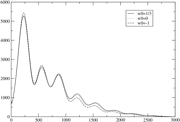
Figure 2: We show the effect of the radiation on the CMB era for $N<N_{i}$ by changing $w=1/3,0,-1$ with $\Delta N_{T}=2\Delta N_{2}=9$.

In fig.(2) we show the different CMB for $w=1/3,0,-1$ for $\Delta N_{T}=N_{o}-N_{i}=9,\Delta N_{2}=N_{2}-N_{1}=4.5$ and $\Delta N_{o}=N_{o}-N_{2}=0$. We have chosen $\Delta N_{T}=9$ because it is the smallest value satisfying the condition $\Delta N_{1}=\Delta N_{2},\Delta N_{o}=0$ and giving the correct CMB spectrum. We have taken $w=1,-1$ for $N_{i}<N<N_{1}$ and $N_{1}<N<N_{2}=N_{o}$, respectively.

We see that the first and second peaks are suppressed for $w=1/3$ compared to $w=-1$ while the third peak is enhanced. The positions of the first two peaks is basically the same and the position of the third peak is moved from 868 to 864 ($0.4\%$), for $w=1/3,-1$ respectively. For smaller $N_{i}$, i.e. more distant from present day, the effect is suppressed. It is not surprising since the $N_{i}$ would be further way from energy-matter equality and its effect on CMB would be less important.

6.2 Effect of First Period, $w=1$

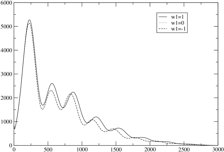
Figure 3: We show the effect of the kinetic era with $N_{i}<N<N_{1}$ by varying $w=1,0,-1$ and $\Delta N_{T}=2\Delta N_{2}=9$. The vertical axes is $l(l+1)c_{l}/2\pi(\mu K^{2})$.

In fig.(3) we show the CMB for different values of $w=1,0,-1$ during $N_{i}<N<N_{1}$ and take $w=1/3$ for $N<N_{i}$ while $w=-1$ for $N_{1}<N_{2}=N_{o}$. The effect of having a kinetic period enhances the first three peaks and shifts the spectrum to higher modes, i.e. higher $l$. The curve for $w=0$ is indistinguishable from the $w=-1$ one. The position and hight of the peaks are $p_{1}=(227,5275),p_{2}=(559,2605),p_{3}=(868,2240)$ for $w=1$ while for $w=-1$ we have $p_{1}=(224,5138),p_{2}=(545,2310),p_{3}=(832,2165)$ giving a percentage difference $p_{1}=(1.3\%,2.6\%),p_{2}=(2.5\%,12.7\%),p_{3}=(4.3\%,3.4\%)$. We see that the largest discrepancy is the altitude of the second peak.

The difference in hight and positions may in principle distinguish between a cosmological constant and a scalar field, or any fluid with the specific equation of state behavior.

The effect of having $w\neq-1$ during $N_{i}<N<N_{1}$ is not significant for $w=0$ and would be even less for a tracker fields with $w_{tr}=cte<-2/3$ but it is observable for $w=1/3$.

6.3 Equal length periods, $\Delta N_{1}\equiv N_{1}-N_{i}=N_{2}-N_{1}\equiv\Delta N_{2},\;\Delta N_{o}\equiv N_{o}-N_{2}=0$

We have studied the case with $\Delta N_{1}=\Delta N_{2},\;\Delta N_{o}=0$. In fig.(4) we show the behavior for different values of $\Delta N_{T}=2\Delta N_{2}=6,8,9,12,16$.

There is a lower limit of $\Delta N_{T}$ that gives an acceptable CMB spectrum. The lower limit is $\Delta N_{T}\geq 9$. For smaller $\Delta N_{T}$ the peaks move to the right of the spectrum and the hight increases giving a spectrum not consistent with the CMB data.

For larger $\Delta N_{T}>9$ the curves tend to the cosmological constant. It is not surprising since for large $\Delta N_{T}=2\Delta N_{2}$ it means that we have a larger time with $w=-1$ and in the case that $\Delta N_{2}>N_{o}-N_{rm}$ the universe content, after matter radiation equality, would have been given by matter and a fluid with $w=-1$, i.e. a cosmological constant.

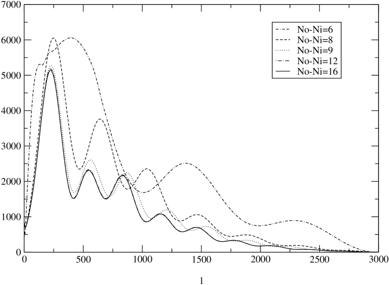
Figure 4: We show the effect on the CMB by varying the $\Delta N_{1}=\Delta N_{2}=3,4,4.5,6.8$ with $\Delta N_{o}=0$. The vertical axes is $l(l+1)c_{l}/2\pi(\mu K^{2})$.

6.4 Scaling condition $\Omega_{\phi}(N_{i})=\Omega_{\phi}(N_{2})=0.1$

Following the discussion in sec.(4.1), we now that a scalar field will end up its scaling period with a $\Omega_{\phi}$ equal to its starting value, i.e. $\Omega_{\phi}(N_{i})=\Omega_{\phi}(N_{2})=0.1$. We have taken this value of $\Omega_{\phi}$ since for $N>N_{i}$ the energy density behaved as radiation and we have to impose the nucleosynthesis bound on relativistic degrees of freedom $\Omega_{\phi}(NS)\leq 0.1-0.2$. Imposing this condition we have determined the evolution of the CMB for three different values of $w_{tr}=-1,-0.82,-0.7$. We have chosen to analyze the $w_{tr}=-0.82$ because it was found to be the best fit tracker model by [8]. We have $w=1/3$ for $N\leq N_{i}$, $w=1$ for $N_{i}\leq N\leq N_{1}$, $w=-1$ for $N_{1}\leq N\leq N_{2}$ and $w=w_{tr}$ for $N_{2}\leq N\leq N_{o}$. The value of $N_{2}$ is determined so that the energy density grows from $\Omega_{\phi}(N_{2})=0.1$ to $\Omega_{\phi}=0.7$ today. This conditions sets the range of the period to $N_{o}-N_{2}=1.03,1.25,1.47$ for $w=-1,-0.82,-0.7$ respectively.

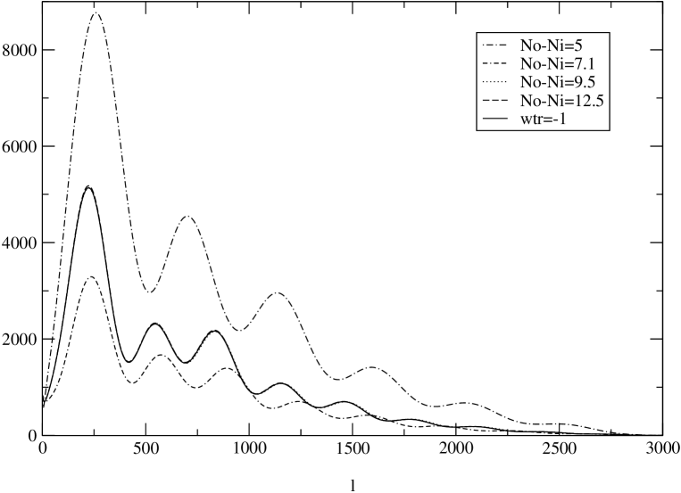
Figure 5: We show the effect on the CMB by varying the $\Delta N_{T}=N_{o}-N_{i}=5,7.1,9.5,12.5$, with the constrain $\Omega_{\phi i}(N_{i})=\Omega_{\phi}(N_{2})=0.1$ and $w_{\phi tr}=-1,\Delta N_{2}=1.03$ and we include the cosmological constant $w\equiv-1$, for comparison. The vertical axes is $l(l+1)c_{l}/2\pi(\mu K^{2})$.

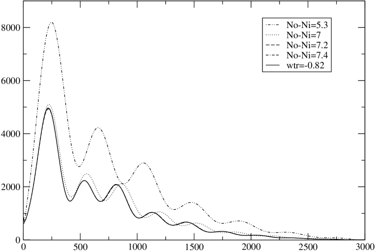
Figure 6: We show the effect on the CMB by varying the $\Delta N_{T}=N_{o}-N_{i}=5.3,7,7.2,7.4$, with the constrain $\Omega_{\phi i}(N_{i})=\Omega_{\phi}(N_{2})=0.1$ and $w_{\phi tr}=-0.82,\Delta N_{2}=1.25$. We also include the tracker with constant $w\equiv=0.82$ The vertical axes is $l(l+1)c_{l}/2\pi(\mu K^{2})$.

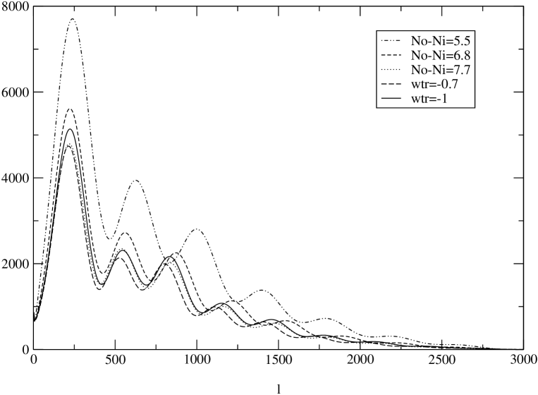
Figure 7: We show the effect on the CMB by varying the $\Delta N_{T}=N_{o}-N_{i}=5.5,6.8,7.7$, with the constrain $\Omega_{\phi i}(N_{i})=\Omega_{\phi}(N_{2})=0.1$ and $w_{\phi tr}=-0.7,\Delta N_{2}=1.47$. We also include the tracker $w=-0.7$ and the constant $w=-1$. The vertical axes is $l(l+1)c_{l}/2\pi(\mu K^{2})$.

In fig.(5),(6) and (7) we show the curves for different values of $N_{i}$ with the restriction that $\Omega_{\phi}(N_{i})=\Omega_{\phi}(N_{2})=0.1$ and for $w_{\phi}=-1,-0.82,-0.7$, respectively.

In the case of $w=-1$ we have $\Delta N_{o}=1.03$ and that the smallest acceptable model has $\Delta N_{T}=8.5$, $\Delta N_{2}=3.6$, see fig.(5). The best model has $\Delta N_{T}=8.88,N_{1}-N_{o}=3.7$ and peaks $p_{1}=(224,5133),p_{2}=(549,2363),p_{3}=(840,2178)$.

For $w=-0.82$, fig.(6), the best fit for tracker models, we have $\Delta N_{o}=N_{o}-N_{2}=1.25$ and the minimum acceptable distance is $\Delta N_{T}=N_{i}-N_{o}=7.19,\Delta N_{2}=3.9$. Smaller values of $\Delta N_{T}$ give a spectrum with peaks too large and second and third peaks moved to the right (high $l$ modes). For large $\Delta N_{T}$ the spectrum tends to the tracker spectrum $w=-0.82$.

The best model has $\Delta N_{T}=N_{1}-N_{o}=7.6,\Delta N_{2}=3.1$ with peaks and position $p_{1}=(223,5016),p_{2}=(551,2450),p_{3}=(851,2102)$. We have compared the $\chi^{2}$ of the models and the $\Delta N_{T}=7.6,w_{\phi}=-0.82$ model has a better fit than the tracker model with constant $w_{tr}=-0.82$, which was found to be the best tracker fit [8]. We see that having a dynamical $w$, is not only more reasonable from a theoretical point of view but it fits the data better.

Finally, we consider $w=-0.7$ for $N>N_{2}$. In this case we have $\Delta N_{o}=N_{o}-N_{2}=1.47$ and the minimum acceptable model has $\Delta N_{T}=6.8,\Delta N_{2}=3.6$, while the best model has $\Delta N_{T}=7.3,\Delta N_{2}=3.8$ with peaks $p_{1}=(222,4954),p_{2}=(550,2422),p_{3}=(853,2035)$.

We see that in all three cases $w=-1,-0.82,-0.7$, with condition $\Omega_{\phi}(N_{i})=\Omega_{\phi}(N_{2})=0.1$ we have a minimum acceptable value of $\Delta N_{T}$ and for smaller $\Delta N_{T}$ the peaks move to the right of the spectrum and the hight of the peaks increases considerably. This conclusion is generic and sets a lower limit to $\Delta N_{T}$, the distance to the phase transition scale $\Lambda_{c}$, or equivalently it sets a lower limit to $\Lambda_{c}$.

The smallest $\Delta N_{T}$ is set by the largest acceptable $w_{\phi o}$ (here we have taken it to be $w_{\phi o}=-0.7$) giving in our case a $\Delta N_{T}=6.8$ for $\Omega_{\phi i}=0.1$. This result puts a constraint on how late the phase transition can take place. In terms of the energy $\Lambda_{c}=\rho_{\phi i}^{1/4}=[\Omega_{\phi i}3H^{2}_{i}]^{1/4}$ we can set a lower value for the transition scale. Using eq.(34) with $\Omega_{\phi i}=0.1$ and$\Delta N_{T}=6.82$ we get

$$\Lambda_{c}=\rho_{\phi i}^{1/4}=2\times 10^{-10}GeV=0.2eV$$ (35)

i.e. for models with a phase transition below eq.(35) the CMB will not agree with the observations. This result is independent of the type of potential.

Furthermore, we now that for inverse power potential there is un upper limit to $\Lambda_{c}$ coming by requiring that $w_{\phi o}<-2/3$. The limiting value assuming $\Omega_{\phi i}\leq 0.1$, for $V=\Lambda^{4+n}\phi^{-n}$, is $n<1.8$ giving $\Lambda_{c}=4\times 10^{-3}GeV\simeq H_{o}^{2/(4+n)}$. Therefore, for IPL potentials the only acceptable models have phase transition scale

$$4\times 10^{-3}GeV>\Lambda_{c}>2\times 10^{-10}GeV.$$ (36)

7 Conclusions

We have analyzed the CMB spectra for a fluid with an equation of state that takes different values. The values are $w=1/3,1,-1,w_{tr}$ for $N$ in the regions $N_{i}-N_{Planck},N_{1}-N_{i},N_{2}-N_{1},N_{o}-N_{2}$, respectively. The results are independent of the type of fluid we have. The cosmological constant and the tracker models are special cases of our general set up.

We have shown that the evolution of a scalar field, for any potential that leads to an accelerating universe at late times, has exactly the kind of behavior described above. It starts at the condensation scale $\Lambda_{c}$ and enters a period with $w=1$, then it undergoes a period with $w=-1$ and finally ends up in a region with $-1\leq w\leq-2/3$. We have shown that the energy density at the end of the scaling period (end of $w=-1$ region) has the same energy ratio as in the beginning, i.e. $\Omega_{\phi}(N_{i})=\Omega_{\phi}(N_{2})$. The time it spends on the last region depends on the value of $\Omega_{\phi}(N_{2})$ and on $w$ during this time. Before the phase transition scale $\Lambda_{c}$ we are assuming that all particles were at thermal equilibrium and massless in the quintessence sector. At the phase transition scale $\Lambda_{c}$ the particles acquire a mass and a non trivial potential.

We have shown that models with $w=1/3,1,-1,w_{tr}$ have a better fit to the data then tracker or cosmological constant. Furthermore, we have determined the effect of the first two periods $w=1/3$ and $w=1$ and even though the effect is small it is nonetheless observable.

In general, the CMB spectrum sets a lower limit to $\Delta N_{T}$, which implies a lower limit to the phase transition scale $\Lambda_{c}$. For smaller $\Delta N_{T}$ the CMB peaks are moved to the right of the spectrum and the hight increases considerably.

For any $\Omega_{\phi i}$ the CMB sets a lower limit to the phase transition scale. In the case of $\Omega_{\phi i}(N_{i})=0.1$ the limit is $\Lambda_{c}=0.2eV$ for any scalar potential. We do not take $\Omega_{\phi i}$ much larger because we should comply with the NS bound on relativistic degrees of freedom $\Omega_{\phi i}\leq 0.1-0.2$. If we take $\Omega_{\phi i}\ll 0.1$ then the constrain on the phase transition scale will be less stringent since the effect of the scalar field is only relevant recently ($\Omega_{\phi}\ll 1$ during all the time before present time).

For inverse power law potentials we can also set un upper limit to $\Lambda_{c}$ and for $\Omega_{\phi i}\leq 0.1$ it gives an inverse power $n\leq 1.8$ and $\Lambda_{c}\leq 4\times 10^{-3}GeV$. In this class of potentials only models with $4\times 10^{-3}GeV>\Lambda_{c}>2\times 10^{-8}GeV$ would give the correct $w_{\phi o}$ and CMB spectrum.

Acknowledgments

We would like to thank useful discussions with C. Terrero. This work was supported in part by CONACYT project 32415-E and DGAPA, UNAM project IN-110200.

References

• [1]
• [2]
• [3] P. de Bernardis et al. Nature, (London) 404, (2000) 955, S. Hannany et al.,Astrophys.J.545 (2000) L1-L4
• [4] A.G. Riess et al., Astron. J. 116 (1998) 1009; S. Perlmutter et al, ApJ 517 (1999) 565; P.M. Garnavich et al, Ap.J 509 (1998) 74.
• [5] G. Efstathiou, S. Maddox and W. Sutherland, Nature 348 (1990) 705. J. Primack and A. Klypin, Nucl. Phys. Proc. Suppl. 51 B, (1996), 30
• [6] P.S. Corasaniti astro-ph/0210257;P.S. Corasaniti, E.J. Copeland astro-ph/0205544,S. Hannestad, E. Mortsell Phys.Rev.D66:063508,2002; J. P. Kneller, G. Steigman astro-ph/0210500
• [7] S. Perlmutter, M. Turner and M. J. White, Phys.Rev.Lett.83:670-673, 1999; T. Saini, S. Raychaudhury, V. Sahni and A.A. Starobinsky, Phys.Rev.Lett.85:1162-1165,2000
• [8] Carlo Baccigalupi, Amedeo Balbi, Sabino Matarrese, Francesca Perrotta, Nicola Vittorio, Phys.Rev. D65 (2002) 063520
• [9] Michael Doran, Matthew J. Lilley, Jan Schwindt, Christof Wetterich, astro-ph/0012139; Michael Doran, Matthew Lilley, Christof Wetterich astro-ph/0105457
• [10] P.S. Corasaniti, E.J. Copeland, Phys.Rev.D65:043004,2002
• [11] I. Zlatev, L. Wang and P.J. Steinhardt, Phys. Rev. Lett.82 (1999) 8960; Phys. Rev. D59 (1999)123504
• [12] A. de la Macorra and C. Stephan-Otto, Phys.Rev.Lett.87:271301,2001
• [13] A.R. Liddle and R.J. Scherrer, Phys.Rev. D59, (1999)023509
• [14] A. de la Macorra and G. Piccinelli, Phys. Rev.D61 (2000) 123503
• [15] E.J. Copeland, A. Liddle and D. Wands, Phys. Rev. D57 (1998) 4686
• [16] P. Brax, J. Martin, Phys.Rev.D61:103502,2000
• [17] E.Kolb and M.S Turner,The Early Universe, Edit. Addison Wesley 1990
• [18] A. de la Macorra hep-ph/0111292
• [19] K. Freese, F.C. Adams, J.A. Frieman and E. Mottola, Nucl. Phys. B 287 (1987) 797; M. Birkel and S. Sarkar, Astropart. Phys. 6 (1997) 197.
• [20] C. Wetterich, Nucl. Phys. B302 (1988) 302, R.H. Cyburt, B.D. Fields, K. A. Olive, Astropart.Phys.17:87-100,2002
• [21] A. de la Macorra, Int.J.Mod.Phys.D9 (2000) 661
• [22] A. de la Macorra and C. Stephan-Otto, Phys.Rev.D65:083520,2002