Chandra X-Ray Observatory observations of the globular cluster M28
and its millisecond pulsar PSR B1821$-$24

Abstract

We report here the results of the first Chandra X-Ray Observatory observations of the globular cluster M28 (NGC 6626). We detect 46 X-ray sources of which 12 lie within one core radius of the center. We show that the apparently extended X-ray core emission seen with the ROSAT HRI is due to the superposition of multiple discrete sources for which we determine the X-ray luminosity function down to a limit of about $6\times 10^{30}$ erg s^-1. We measure the radial distribution of the X-ray sources and fit it to a King profile finding a core radius of $r_{c,x}\approx 11\arcsec$. We measure for the first time the unconfused phase-averaged X-ray spectrum of the 3.05-ms pulsar B1821$-$24 and find it is best described by a power law with photon index $\Gamma\simeq 1.2$. We find marginal evidence of an emission line centered at 3.3 keV in the pulsar spectrum, which could be interpreted as cyclotron emission from a corona above the pulsar’s polar cap if the the magnetic field is strongly different from a centered dipole. The unabsorbed pulsar flux in the 0.5–8.0 keV band is $\approx 3.5\times 10^{-13}\,{\rm ergs\,\,s}^{-1}\,{\rm cm}^{-2}$. We present spectral analyses of the 5 brightest unidentified sources. Based on the spectral parameters of the brightest of these sources, we suggest that it is a transiently accreting neutron star in a low-mass X-ray binary, in quiescence. Fitting its spectrum with a hydrogen neutron star atmosphere model yields the effective temperature $T_{\rm eff}^{\infty}=90^{+30}_{-10}$ eV and the radius $R_{\rm NS}^{\infty}=14.5^{+6.9}_{-3.8}$ km. In addition to the resolved sources, we detect fainter, unresolved X-ray emission from the central core. Using the Chandra-derived positions, we also report on the result of searching archival Hubble Space Telescope data for possible optical counterparts.

1 Introduction

Since the Einstein era it has been clear that globular clusters contain various populations of X-ray sources of very different luminosities (Hertz & Grindlay 1983). The stronger sources ($L_{x}\approx 10^{36}-10^{38}$ ${\rm erg}\,{\rm s}^{-1}$) were seen to exhibit X-ray bursts which led to their identification as low-mass X-ray binaries (LMXBs). The nature of the weaker sources, with $L_{x}\leq 3\!\times\!10^{34}$ ${\rm erg}\,{\rm s}^{-1}$, however was more open to discussion (e.g., Cool et al. 1993; Johnston & Verbunt 1996). Although many weak X-ray sources were detected in globulars by ROSAT (Johnston & Verbunt 1996; Verbunt 2001), their identification has been difficult due to low photon statistics and strong source confusion in the crowded globular cluster fields, except for a few cases (Cool et al. 1995 and Grindlay et al. 1995). The application of the Chandra X-Ray Observatory (CXO) sub-arcsecond angular resolution to the study of globular cluster X-ray sources leads one to anticipate progress in our understanding.

Advances with the CXO have already included observations of NGC 6752 (Pooley et al. 2002a), 6440 (Pooley et al. 2002b), 6397 (Grindlay et al. 2001) and 5139 (Rutledge et al. 2002a) which detected more low-luminosity X-ray sources than in all ROSAT observations of 55 globular clusters combined. Of particular interest are the results obtained from CXO observations of 47 Tuc = NGC 104. Grindlay et al. (2001) reported the detection of 108 sources within a region corresponding to about 5 times the 47 Tuc core radius. Sixteen of the soft/faint sources were found to be coincident with radio-detected millisecond pulsars (MSPs), and Grindlay et al. (2001, 2002) concluded that more than 50 percent of all the unidentified sources in 47 Tuc are MSPs. This conclusion is in concert with theoretical estimates on the formation scenarios of short-period (binary) pulsars in globular clusters (Rasio, Pfahl & Rappaport 2000).

The globular cluster M28 = NGC 6626 lies close to the galactic plane ($b=-5.58\arcdeg$) and close to the galactic center ($l=7.8\arcdeg$) (Harris 1996). Distance estimates for M28 range from 5.1 kpc (Rees & Cudworth 1991) to 5.7 kpc (Harris 1996). In this paper, we use 5.5 kpc as a reference distance.

M28 is a relatively compact cluster with a core radius of 0$\farcm$24, corresponding to $r_{c}\sim 0.4$ pc, and a half-mass radius of 1$\farcm$56, corresponding to $\sim$2.6 pc (Harris 1996). The values of these radii in parsec are smaller than those for the better studied 47 Tuc. Thus, although M28’s central luminosity density, $\rho_{0}=10^{4.75}\,\,L_{\odot}\,\,{\rm pc}^{-3}$, is comparable to that of 47 Tuc ($10^{4.77}\,\,L_{\odot}\,\,{\rm pc}^{-3}$ — Harris 1996), the rate of two-body encounters in the core, $N_{\rm enc}\propto\rho_{0}^{1.5}r_{c}^{2}$, is a factor of $2$ smaller, and thus fewer binaries are created and expected as dim X-ray sources .

Davidge, Cote & Harris (1996) noted that M28’s position in the plane near the galactic center and its relative compactness may indicate that it has been in the inner Galaxy for a long time. The authors suggest an age of $\sim$16 Gyr. This age, however, seems to be too high compared with the recent results by Salaris & Weiss (2002) and Testa et al. (2001) from which one estimates the age of M28 to be $11.4-11.7$ Gyr, consistent with M28’s moderately low metallicity [Fe/H]$=-1.45$.

The absorbing column towards M28 is $\sim$10 times larger than for 47 Tuc, with reddening E$(B-V)=0.43$ (Harris 1996) corresponding to a hydrogen column density $N_{H}\sim 2.4\times 10^{21}$ cm^-2.

The first millisecond pulsar discovered in a globular cluster was PSR B1821$-$24 in M28 (Lyne et al. 1987). This solitary MSP has a rotation period of $P=3.05$ ms and period derivative of $\dot{{P}}=1.61\times 10^{-18}$ s s^-1. This value for the period derivative is sufficiently large that the expected correction due to line-of-sight projection of acceleration in the cluster’s gravitational potential (Phinney 1993) is $\lesssim$10% (assuming a $10^{\prime\prime}$ projected offset from the cluster center and a cluster core mass $\sim 10^{4}$ M_⊙; this assumed core mass is slightly higher than that derived from the values for central luminosity density and core radius given by Harris 1996). Therefore, the measured value reasonably accurately reflects the pulsar’s intrinsic period derivative. The inferred pulsar parameters make it the youngest ($P/2\dot{P}=3.0\times 10^{7}$ yrs) and most powerful ($\dot{E}=2.24\times 10^{36}I_{45}$ erg s^-1) pulsar among all known MSPs. Here $I_{45}$ is the neutron star moment of inertia in units of $10^{45}$ g cm². For the idealized magnetic dipole radiation model, the inferred perpendicular component of the magnetic dipole moment is $\mu\,\sin\alpha=3.2\times 10^{37}(I_{45}P\dot{P})^{1/2}=2.2\times 10^{27}I_{45}^{1/2}$ G cm³, where $\mu$ is the magnetic dipole moment and $\alpha$ the angle between the rotation and magnetic dipole axes. Neglecting higher multipole contributions to the magnetic field and assuming the magnetic moment to be at the neutron star center, the inferred magnitude of the dipolar field at the magnetic pole is $B_{p}=4.5\times 10^{9}\,I_{45}^{1/2}R_{6}^{-3}(\sin\alpha)^{-1}$ G, where $R_{6}$ is the neutron star radius in units of $10^{6}$ cm. Although these values for the dipole moment and polar dipole field are about 2 orders of magnitude smaller than what is inferred for ordinary field pulsars in the galactic plane, they are the highest among all MSPs. The pulsar’s high rotational-energy loss made PSR B1821$-$24  a prime candidate to be a rotationally powered, non-thermal X-ray source. This was confirmed by X-ray observations performed with different X-ray satellites, e.g., ROSAT (Danner et al. 1997 — cf. Verbunt 2001), ASCA (Saito et al. 1997) and RXTE (Rots et al.  1998), which detected Crab-like pulsations.

While the detection of strongly pulsed emission would suggest a magnetospheric origin of the X-ray emission, a clear characterization of the PSR B1821$-$24 spectrum has been hampered so far by the crowding of sources in the region. Indeed, observation of M28 with the ROSAT HRI made it clear that all spectral data obtained from PSR B1821$-$24, especially in the “soft” bands $\leq 10$ keV, suffer from spectral contamination from nearby sources. Stretching the angular resolution of the HRI to its limit, four X-ray sources within 2′ of the cluster center were discovered, including the two barely resolved sources RX J1824.5$-$2452E and RX J1824$-$2452P located within 15″ of the center of M28, with the latter being identified from the timing as the counterpart of the millisecond pulsar B1821$-$42.

Danner et al. (1997) put forth the suggestions that the $\sim 10^{\prime\prime}\times 10\arcsec$ extended region of emission associated with RX J1824.5–2452E was due to either a synchrotron nebula powered by the pulsar or a number of faint LMXBs. The latter interpretation was favored as measurements with the ROSAT PSPC exhibited flux variations by as much as a factor of 3 between observations performed in 1991 and 1995 (see also Becker & Trümper 1999). Further evidence was provided by Verbunt (2001) who reanalyzed the ROSAT HRI data and resolved RX J1824.5$-$2452E into at least 2 sources. Time variations of the sources in M28 are also compatible with the result of Gotthelf & Kulkarni (1997) who discovered an unusually subluminous ($L_{x}\approx 10^{-2}L_{\rm Edd}$) “Type I” X-ray burst from the direction of M28, thus leading one to expect the presence of one or more LMXBs.

In this paper we report on the first deep X-ray observations of M28 using the ACIS-S detector aboard the CXO. We show that the X-ray core emission seen with the ROSAT HRI is dominated by a superposition of multiple discrete sources; we measure the unconfused phase-averaged spectrum of the X-ray flux from the 3.05-ms PSR B1821$-$24; we establish the X-ray luminosity function down to a limit of about $6\times 10^{31}$ erg s^-1 and measure, with high precision, the absolute positions of all the detected X-ray sources in M28 to facilitate identifications in other wavelength bands. Observations and data analysis are described in §2.1 through §2.3. In addition, we have used archival Hubble Space Telescope (HST) observations to search for potential optical counterparts of the sources detected by the CXO (§3).

2 Observations and data analysis

M28 was observed three times for approximately equal observing intervals of about 13 ksec between July and September 2002 (Table 1). These observations were scheduled so as to be sensitive to time variability on time scales up to weeks. The observations were made using 3 of the CXO Advanced CCD Imaging Spectrometer (ACIS) CCDs (S2,3,4) in the faint timed exposure mode with a frame time of 3.241 s. Standard Chandra X-Ray Center (CXC) processing (v.6.8.0) has applied aspect corrections and compensated for spacecraft dither. Level 2 event lists were used in our analyses. Events in pulse invariant channels corresponding to $\approx 0.2$ to 8.0 keV were selected for the purpose of finding sources. Due to uncertainties in the low energy response, data in the range 0.5 to 8.0 keV were used for spectral analyses. Increased background corrupted a small portion of the third data set reducing the effective exposure time from 14.1 ksec to 11.4 ksec (Table 1) although no results were impacted by the increased background.

The optical center of the cluster at $\alpha_{2000}=18^{\rm h}\,24^{\rm m}\,32\fs 89$ and $\delta_{2000}=-24\arcdeg\,52\arcmin\,11\farcs 4$ (Shawl and White 1986) was positioned 1′ off-axis to the nominal aim point on the back-illuminated CCD, ACIS-S3, in all 3 observations. A circular region with 3$\farcm$1-radius, corresponding to twice the half-mass radius of M28, centered at the optical center was extracted from each data set for analysis. No correction for exposure was deemed necessary because the small region of interest lies far from the edges of the S3 chip.

The X-ray position of PSR B1821$-$24 was measured separately using the three data sets and the merged data. The results of these measurements are listed in Table 2. The set-averaged position is the same as that derived using the merged data set. The root-mean-square (rms) uncertainty in the pulsar position, based on the 3 pointings, is 0$\farcs$042 in right ascension and 0$\farcs$029 in declination. The radio position and proper motion of the pulsar, as measured by Rutledge et al. (2003), places the pulsar at the time of the observation only $\Delta_{\alpha}=$ 0$\farcs$083, $\Delta_{\delta}=-0\farcs 042$ away from the best-estimated X-ray position. In what follows the observed X-ray positions of all sources have been adjusted to remove this offset.

2.1 Image Analysis

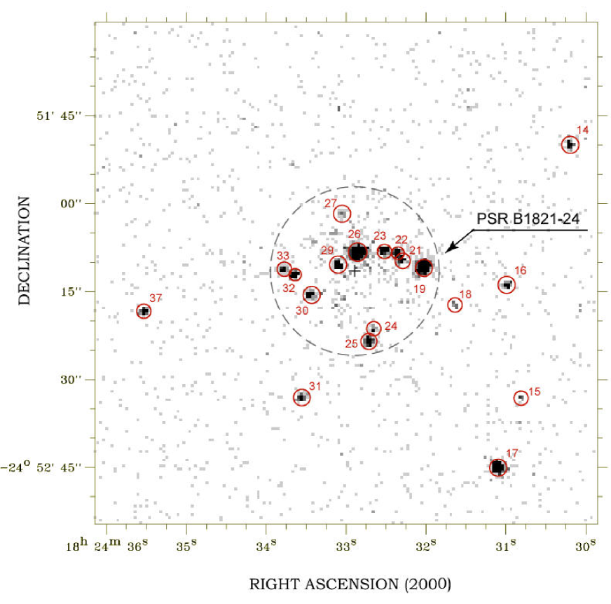
Figure 1: CXO ACIS-S3 image of the central region of M28. Twelve X-ray sources are detected within the 0$\farcm$24 core-radius, indicated by a dashed circle. The optical center of the cluster is indicated by a cross. The X-ray counterpart of the millisecond pulsar B1821–24 is source #19.

The central portion of the combined CXO image is shown in Figure 1. We used the same source finding techniques as described in Swartz et al. (2002) with the circular-gaussian approximation to the point spread function, and a minimum signal-to-noise (S/N) ratio of 2.6 resulting in much less than 1 accidental detection in the field. The corresponding background-subtracted point source detection limit is $\sim$10 counts. The source detection process was repeated using the CXC source detection tool wavdetect (Freeman et al. 2002) and yielded consistent results at the equivalent significance level. Forty-four sources were found using these detection algorithms. Close inspection of the image with the source positions overlaid and of the source time variations showed that one source detected by the software was really two sources (numbers 21 and 22 of Fig. 1), and that an additional source, # 24, is also present.

Table 3 lists the 46 X-ray sources. The table gives the source positions, the associated uncertainty in these positions, the radial distance of the source from the optical center, the signal-to-noise ratio, the aperture-corrected counting rates in various energy bands, the unabsorbed luminosity in the $0.5-8.0$ keV energy range based on the spectroscopy discussed in § 2.2, and a variability designation according to the discussion in § 2.3.

The positional uncertainty listed in column 4 of Table 3 is given by $r=1.51(\sigma^{2}/N+\sigma_{o})^{1/2}$ where $\sigma$ is the size of the circular gaussian that approximately matches the PSF at the source location, $N$ is the aperture-corrected number of source counts, and $\sigma_{o}$ represents the systematic error. Uncertainties in the plate scale imply a systematic uncertainty of $0\farcs 13$, and, given that the radio and CXO positions agree to $0\farcs 2$, we feel that using $0\farcs 2$ is a reasonable and conservative estimate for $\sigma_{o}$. The factor 1.51 is the radius that encloses 68% of the circular gaussian. The parameter $\sigma$, varies from $\sim 0\farcs 9$ near the aimpoint to $<2\farcs 1$ near the edge of the $3\farcm 1$-radius extraction region.

The rates in the soft, medium, and hard bands listed in Table 3 are background subtracted and have (asymmetrical) 67% confidence uncertainties based on Poisson statistics (rather than the usual symmetrical Gaussian approximation). When the band-limited rates are positive, the uncertainties are symmetrical in probability space (that is we set the lower and upper limits to the 67% confidence interval so that the true source rate is equally likely to fall on either side of the derived rate), but not in rate space. Otherwise, we set the rate to zero and calculate a 67% upper limit.

From Figure 1 we see that there are 12 point sources in the central region in the summed image. In addition, there remains some unresolved emission from this region of the cluster (§ 2.2.5). Pooley et al. (2002b) found similar diffuse emission in the central regions of the CXO image of the globular cluster NGC 6440.

2.1.1 Radial Distribution

The projected surface density, $S(r)$, of detected X-ray sources was compared to a King profile, $S(r)=S_{o}[1+(r/r_{o})^{2}]^{-\beta}+C_{0}$. The constant term $C_{0}$ was added to account for background sources. We estimated the number of background sources using our observed flux limits of $\sim 5.5\times 10^{-16}$ ergs cm^-2 s^-1 in the 0.5–2.0 keV band and $\sim 1.5\times 10^{-15}$ ergs cm^-2 s^-1 in the 2.0–10 keV band. These limits, together with the $\log N(>S)$-$\log S$ distribution from the CXO Deep Field South (Rosati et al. 2002) gives an estimate of at least $\sim$0.3 to 0.4 background sources per square arcmin in the field. (The true value may be higher because of the low galactic latitude of M28 relative to the deep field.) The best-fit value for $C_{o}$ is $0.36\pm 0.22$ sources per arcmin² indicating that there are $\sim 10$ sources in the $3\arcmin$-radius field not associated with the cluster. The other fit parameters ($S_{o}=123\pm 11$ sources per arcmin², $r_{0}=23\farcs 8^{+10.8}_{-5.9}$, $\beta=3.51^{+2.7}_{-1.1}$) can be used to estimate the core radius, $r_{c,x}$, and the typical mass, $M_{x}$, of the X-ray source population. We find a best fit core radius $r_{c,x}=10\farcs 9^{+8.8}_{-4.7}$. This is comparable to the distribution of optical light of the cluster: $r_{c\ast}=14\farcs 4$ (Harris 1996). Following the derivation of Grindlay et al. (2002), the best-fit mass of the X-ray sources is $M_{x}=1.87^{+1.25}_{-0.49}$ M_⊙, assuming the dominant visible stellar population has a mass of $M_{\ast}\sim 0.7$ M_⊙. Although our range for $M_{x}$, estimated in this way, barely overlaps the range $1.1-1.4$ M_⊙ deduced by Grindlay et al.  (2002) for 47 Tuc, additional effects due to uncertainties in cluster properties (position of cluster center, core radius, mass segregation, etc.) mean that the two results are in fact indistinguishable.

2.2 Spectral Analysis

Point-source counts and spectra were extracted from within radii listed in Table 4. Because the field is so crowded, background was estimated using a region of $\sim 50\arcsec$ radius located in the south-western portion of the field. The background rate, used for all calculations, was $3.7\times 10^{-6}$ counts s^-1 arcsec^-2.

Only 6 of the 46 detected sources have sufficient counts to warrant an individual spectral analysis. In descending order of the number of detected counts these are sources #26, #19, #4, #17, #25, and #28. Source #19 is the X-ray counterpart of the PSR B1821–24. The results of fitting various spectral models to the energy spectra of the brightest sources are presented in § 2.2.1, § 2.2.2, and § 2.2.3. All spectral analyses used the CXC CALDB 2.8 calibration files (gain maps, quantum efficiency uniformity and effective area). The abundances of, and the cross sections in, TBABS (available in XSPEC v.11.2) by Wilms, Allen & McCray (2000) were used in calculating the impact of the interstellar absorption. All errors are extremes on the single interesting parameter 90% confidence contours.

A correction was applied when fitting models to the spectral data to account for the temporal decrease in low-energy sensitivity of the ACIS detectors due, presumably, to contamination buildup on the ACIS filters. The correction was based on the average time of the observations after launch of 1105 days.

For the remaining 40 sources, all with fewer than 100 detected source counts, the spectra were combined to determine the mean spectral shape and total luminosity. Fits were made using both an absorbed power law ${\rm d}N/{\rm d}E\propto E^{-\Gamma}$ (best-fit $\Gamma=1.73\pm 0.18$, $N_{22}=N_{H}/(10^{22}\,{\rm cm}^{-2})=0.18\pm 0.06$, $\chi^{2}=89.8$ for 86 degrees of freedom (dof)) and an absorbed thermal bremsstrahlung model ($kT=7.40\pm 2.10$ keV, $N_{22}=0.12\pm 0.04$, $\chi^{2}=92.8$). Using the power-law model parameters, the total (unabsorbed) flux from the 40 weak sources is $2.34\pm 0.11\times 10^{-13}$ ergs cm^-2 s^-1 in the 0.5–8.0 keV band, and the corresponding X-ray luminosity is $8.47\pm 0.40\times 10^{32}$ ergs s^-1. This spectrum was then used to estimate the individual source luminosities of the 40 faint sources listed in Table 3. See also the discussion in § 2.2.4.

2.2.1 The Phase-averaged Spectrum of PSR 1821–24

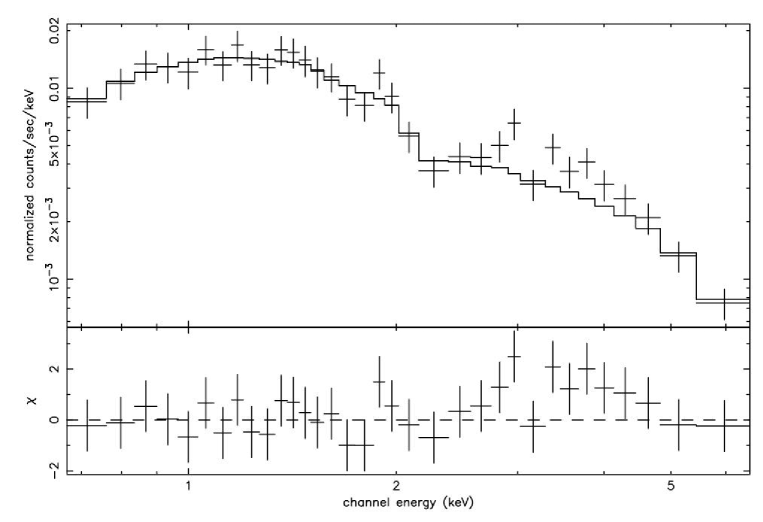
Figure 2: Energy spectrum of the millisecond pulsar PSR B1821$-$24 fit to an absorbed power-law model (upper panel) and contribution to the $\chi^{2}$ fit statistic (lower panel). The residuals indicate a marginally significant feature near 3 keV.

The spectrum of PSR B1821$-$24  was measured by extracting $\sim 1100$ counts within a radius of 1$\farcs$72 centered on the pulsar position. A background subtraction was performed, but its contribution ($\sim 2$ counts) is negligible. Neither our source-detection algorithm nor wavdetect found any evidence for a spatial extent to the pulsar’s X-ray counterpart; thus, using the CXC model point spread function, 97% of all the events from PSR B1821$-$24  are within the selected region. The data were binned into 34 bins guaranteeing at least 30 counts per bin. Model spectra were then compared with the observed spectrum. A power-law model was found to give a statistically adequate representation of the observed energy spectrum; the best-fit spectrum and residuals are shown in Figure 2. A thermal bremsstrahlung model resulted in a slightly better fit, but is not considered to be physically applicable. A blackbody model does not fit the data ($\chi^{2}=110$ for 31 dof), as one could expect based upon the hardness of the observed spectrum and the similarity of the sharp X-ray and radio pulse profiles (see, for example, Becker & Pavlov 2001, Becker & Aschenbach 2002).

The best-fit power law yields $N_{22}=0.16^{+0.07}_{-0.08}$, $\Gamma=1.20^{+0.15}_{-0.13}$, and a normalization of $3.74^{+1.0}_{-0.48}\times 10^{-5}$ photons cm^-2 s^-1 keV^-1 at $E=1$ keV ($\chi_{\nu}^{2}=0.89$ for 31 dof). The column density is in fair agreement with what is deduced from the reddening towards M28. The unabsorbed energy flux in the 0.5–8.0 keV band is $f_{x}=3.54^{+0.06}_{-0.05}\times 10^{-13}\,\,{\rm ergs\,\,s}^{-1}\,{\rm cm}^{-2}$, yielding an X-ray luminosity of $L_{x}=1.28\pm 0.02\times 10^{33}\,{\rm ergs\,\,s}^{-1}$. This luminosity implies a rotational energy to X-ray energy conversion factor $L_{x}/\dot{E}=5.8\times 10^{-4}$. If transformed to the ROSAT band, this corresponds to $L_{x}=(3.4$–$4.0)\times 10^{32}\,{\rm ergs\,\,s}^{-1}$, and is similar to the luminosity inferred from the ROSAT data (Verbunt 2001). The photon index we found is compatible with $\Gamma\sim 1.1$ deduced for PSR B1821$-$24 from the observations at pulse maximum using RXTE data (Kawai & Saito 1999). We note that we have ignored the possible effects of photon pileup, and this could artificially harden the spectral index. However, the degree of pileup here is sufficiently small ($<0.12$ counts per frame), so that its effect on the spectrum is not significant. In fact, application of the Davis (2001) pileup model suggests the spectral index would be steeper by only  0.1 in the absence of pileup.

The residuals in Figure 2 hint at a spectral feature or features at an energy slightly above 3 keV. Although the reduced number of counts made it impossible to determine whether the feature was present in the three separate observations, we note that some excess emission in the band between 3 and 4 keV is seen in all three data sets. By adding a gaussian “line” to the power law model, we found a line center at 3.3 keV with a gaussian width of 0.8 keV and a strength of $\approx 6\times 10^{-6}$ photons cm^-2 s^-1, which corresponds to a luminosity of $\approx 1.1\times 10^{31}\,\,{\rm erg\,s}^{-1}$. Adding the line changes $\chi_{\nu}^{2}$ to 0.63 (for 28 dof). The F-test indicates that the addition of this line component is statistically significant at 98% confidence, i.e., evidence for a broad spectral feature is marginal.

If we assume that this feature is real, then it is interesting to speculate as to its origin. There are some atomic lines, from K and Ar, close to the 3.3 keV energy. However, K is not an abundant element, and it is hard to explain why the Ar lines are observed while no lines are seen from other, more abundant, elements. Therefore, we consider the more likely possibility that this is an electron cyclotron line, formed in a magnetic field $B\approx 3\times 10^{11}$ G. Such a strong field can be explained by the presence of either multipolar components or a strong off-centering of the magnetic dipole or both.

For instance, if a dipole with the magnetic moment $\mu=2\times 10^{27}$ G cm³ (see §1) is shifted along its axis such that it is 1.9 km beneath the surface, the magnetic field at the closest pole is $3\times 10^{11}$ G. The cyclotron line could be formed in an optically thin, hot corona above the pulsar’s polar cap, with a temperature $kT\sim 10$ keV such that the line’s Doppler width is smaller than observed while the excited Landau levels are populated. The observed luminosity in the line can be provided by as few as $N_{e}=2.4\times 10^{25}\,T_{8}^{-1}B_{11.5}^{-2}$ electrons, where $T_{8}=T/(10^{8}\,{\rm K})$, $B_{11.5}=B/(3\times 10^{11}\,{\rm G})$.

The corona is optically thin at the line center for an electron column density $n_{e}H<5\times 10^{18}\,T_{8}^{1/2}B_{11.5}$ cm^-2 (where $H$ is the geometrical thickness of the corona) and a polar cap area $A_{\rm pc}>4.6\times 10^{6}\,T_{8}^{-3/2}B_{11.5}^{-3}$ cm² (polar cap radius $R_{\rm pc}>12$ m). The standard estimate of the polar cap radius, applied to the off-centered dipole, gives $R_{\rm pc}\sim r(2\pi r/cP)^{1/2}=220$ m, where $r$ ($=1.9$ km in our example) is the radial distance from the center of the magnetic dipole to the surface. At this value of $R_{\rm pc}$, the optical thickness at the line center is $\tau\sim 0.003\,T_{8}^{-3/2}B_{11.5}^{-3}$. If the corona is comprised mainly of a proton-electron plasma, then its thickness can be estimated as $H\sim kT\,(m_{H}g)^{-1}\sim 40\,T_{8}$ cm (at $g\sim 2\times 10^{14}$ cm s^-2, typical for a neutron star), and a characteristic electron number density is $n_{e}\sim 5\times 10^{14}\,T_{8}^{-2}B_{11.5}^{-2}$ cm^-3. Thus, the cyclotron interpretation of the putative line looks quite plausible, and confirming the line with deeper observations would provide strong evidence of local magnetic fields at the neutron star surface well above the “conventional” magnitudes inferred from the assumption of the centered dipole geometry.

2.2.2 Source #26: An LMXB in quiescence?

Of particular interest among the brightest X-ray sources detected in M28 is the luminous, soft source #26. We extracted data as per Table 4 and fit it with various spectral models. As expected from the softness of the count spectrum (Fig. 3), the power-law fit yields a photon index, $\Gamma\approx 5.2$, well in excess of those observed from known astrophysical sources with power-law spectra, and the hydrogen column density, $N_{22}\approx 0.68$, that significantly exceeds the values expected from the M28’s reddening (§1) and measured for the pulsar (§2.2.1). Therefore, we tried various models of thermal radiation. A blackbody fit gives the hydrogen column density $N_{22}\approx 0.13$, temperature $kT_{\rm BB}\approx 0.26$ keV and radius $R_{\rm BB}\approx 1.3$ km, corresponding to the bolometric luminosity of $L_{\rm BB}\sim 1\times 10^{33}$ erg s^-1. Such values are typical for blackbody fits of LMXBs with transiently accreting neutron stars in quiescence (e.g., Rutledge et al. 2000). The relatively high temperatures of such old neutron stars can be explained by heating of the neutron star crust during the repeated accretion outbursts (Brown, Bildsten, & Rutledge 1998). This heat provides an emergent thermal luminosity $L=8.7\times 10^{33}\langle\dot{M}\rangle_{-10}$ erg s^-1, for the nuclear energy release of 1.45 MeV per accreted nucleon, where $\langle\dot{M}\rangle_{-10}$ is the time-averaged accretion rate in units of $10^{-10}\,M_{\odot}\,\,{\rm yr}^{-1}$.

The radius $R_{\rm BB}$ obtained from the blackbody fit is much smaller than $R\sim 10-15$ km expected for a neutron star. A likely reason for this discrepancy is that the blackbody model does not provide an adequate description of thermal radiation from the neutron star surface. At the temperatures of interest the neutron star crust is covered by an atmosphere comprised of the accreted matter. Because of the gravitational sedimentation, the outermost layers of such an atmosphere, which determine the properties of the emergent radiation, are comprised of hydrogen, the lightest element present. Since the magnetic fields of neutron stars in LMXBs are expected to be relatively low, $\lesssim 10^{9}$ G, they should not affect the properties of X-ray emission, which allows one to use the nonmagnetic hydrogen atmosphere models (Rajagopal & Romani 1996; Zavlin, Pavlov & Shibanov 1996). We fit the observed spectrum with the nsa model in XSPEC (v.11.2). In applying this model, we set the neutron star mass to 1.4M_⊙, leaving the radius of the emitting region and the surface temperature as free parameters. We obtained a statistically acceptable fit ($\chi_{\nu}^{2}=0.96$, $\nu=44$), with the hydrogen column density $N_{22}=0.26\pm 0.04$ (consistent with the expected value), the effective temperature $kT_{\rm eff}^{\infty}=0.09^{+0.03}_{-0.01}$ keV, a factor of 3 lower than $T_{\rm BB}$, and the radius $R^{\infty}=14.5^{+6.9}_{-3.8}$ km, comparable with a typical neutron star radius. (The superscript ^∞ means that the quantities are given as measured by a distant observer; they are related to the quantities as measured at the neutron star surface as $T^{\infty}=g_{r}T$, $R^{\infty}=g_{r}^{-1}R$, $L_{\rm bol}^{\infty}=g_{r}^{2}L_{\rm bol}$, where $g_{r}=(1-2GM/Rc^{2})^{1/2}$ is the gravitational redshift factor. The values of $T_{\rm eff}^{\infty}$ and $R^{\infty}$, as inferred from the atmosphere model fits, are considerably less sensitive to the assumed value of neutron star mass.)

The corresponding bolometric luminosity is $L_{\rm bol}^{\infty}=1.9^{+1.1}_{-0.6}\times 10^{33}$ erg s^-1. Such a luminosity can be provided by a time-averaged accretion rate of $\langle\dot{M}\rangle\sim 2\times 10^{-11}\,M_{\odot}\,\,{\rm yr}^{-1}$. Because all the fitting parameters we obtained for source #26 are typical for quiescent radiation of other transiently accreting neutron stars in LMXBs (e.g., Rutledge et al. 2002b, and references therein), we conclude that such an interpretation is quite plausible.

In addition to the thermal (photospheric) component, some X-ray transients in quiescence show a power-law high-energy tail (Rutledge et al. 2002b), apparently associated with a residual low-rate accretion. We can see from Figure 3 that our thermal model somewhat underestimates the measured flux above 2.5 keV. This is a consequence of a mild (0.16 counts per frame) amount of pileup. The pileup model suggested by Davis (2001), as implemented in XSPEC v.11.2, does reproduce this tail, but only marginally changed the best-fit parameters.

The quiescent emission of some of transient LMXBs shows appreciable variations of X-ray flux, with a time scale of a month (Rutledge et al. 2002b), and our source #26 also appears to be time variable (§2.3) in the three observations. We performed spectral fits to each of the data sets separately to check for spectral variation and found none, indicating that the time variability (§ 2.3) is not dominated by spectral variations.

To test alternative interpretations of source #26, we also fit various model spectra of an optically thin thermal plasma in collisional equilibrium, applicable to stellar coronae and similar sources. Fitting the spectrum with the XSPEC model mekal, for $Z=0.02Z_{\odot}$, we obtain a good fit ($\chi_{\nu}^{2}=0.88$ for 44 dof) with $N_{22}\approx 0.33$, $kT\approx 0.6$ keV, and emission measure EM $\approx 2\times 10^{57}$ cm^-3, at $d=5.5$ kpc. The corresponding luminosity, $L_{x}(0.5-8\,{\rm keV})\approx 1.2\times 10^{33}$ erg s^-1, strongly exceeds the maximum luminosities of coronal emission observed from either single or multiple nondegenerate stars of any type available in an old globular cluster. The spectrum is too hard, and the luminosity is too high, to interpret this emission as produced by a non-magnetic CV (Warner 1995, and references therein). The inferred temperature is too low in comparison with the typical temperatures, $\sim 30-40$ keV, of the hard X-ray (bremsstrahlung) component observed in polars (magnetic CVs, in which rotation of the accreting magnetic white dwarf is synchronized with the orbital revolution), and, in addition, this component is usually much less luminous in polars. On the other hand, the spectrum of source #26 is too hard to be interpreted as a soft X-ray component ($20-40$ eV blackbody plus cyclotron radiation) observed in many polars. Luminosities up to $\sim 1\times 10^{33}$ erg s^-1 (in the $2-10$ keV band) have been observed in a number of intermediate polars (asynchronous magnetic CVs with disk accretion). However, spectra of intermediate polars are, as a rule, much harder (similar to those observed in polars) and strongly absorbed ($N_{22}\sim 10$) by the accreting matter (Warner 1995). Therefore, we conclude that the interpretation of source #26 as a stellar corona or a CV looks hardly plausible, and most likely its X-ray emission emerges from the photosphere of a quiescent transient neutron star in an LMXB.

2.2.3 Spectra of Four Other Bright Sources

In addition to PSR B1821$-$24 and source #26, there are 4 moderately bright sources with enough counts to attempt spectral fitting. Data from an extraction radius large enough to encompass a significant fraction of the source counts were binned into spectral bins to maintain a minimum number of counts per bin, background subtracted, and fit to various spectral models. The extraction radii, total number of extracted counts, estimated number of background counts, minimum number of counts per spectral bin, and the number of spectral bins are listed in Table 4. To characterize the spectra of these sources, we fit each of them with three popular models of substantially different shapes: a black-body, a power-law, and an optically-thin thermal emission model (mekal) with $Z=0.02\,Z_{\odot}$. The best-fit parameters for these models, including uncertainties, are given in Table 5.

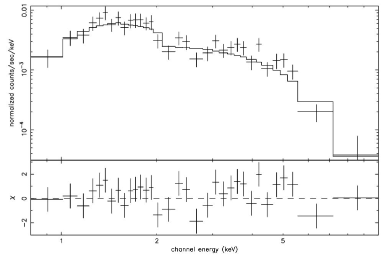
Figure 4: Energy spectrum of source #4, fit with an absorbed power-law model.

The brightest of the four sources is source #4. Its spectrum (Fig. 4) is too hard to consider it as a qLMXB. The power-law fit of the spectrum, with $\Gamma\approx 1.6$, might be interpreted as arising from magnetospheric emission from an MSP, with a luminosity $L_{x}\approx 9\times 10^{32}$ erg s^-1, in the $0.5-8$ keV range. However, the hydrogen column density inferred from the power-law fit, $N_{22}\approx 0.86$, considerably exceeds those estimated from the interstellar reddening and the power-law fit of the PSR B1821$-$24 spectrum. The large $N_{H}$ and a large distance, 2$\farcm$53 from the cluster’s center, together with the power-law slope typical for AGNs, hint that source #4 could be a background AGN (notice that the Galactic HI column density in this direction is about $0.19\times 10^{22}$ cm^-2 — Dickey & Lockman 1990). The blackbody fit gives $N_{22}\approx 0.16$, consistent with that obtained for PSR B1821$-$24. This fit indicates that source #4 might be a thermally emitting MSP, although the blackbody temperature, $\approx 1$ keV, is surprisingly high, and the blackbody radius, $\approx 60$ m, is much smaller than expected for a pulsar polar cap (a standard polar cap radius is $R_{\rm pc}=1.4\,R_{6}^{3/2}P_{-2}^{-1/2}$ km, assuming a centered dipole, where $R_{6}$ is the neutron star radius in units of 10 km, and $P_{-2}$ is the pulsar’s period in units of 10 ms). The inferred temperature would become lower by a factor of two, and the radius would increase by an order of magnitude if we assume that this emission emerges from a polar cap covered by a hydrogen or helium atmosphere (e.g., Zavlin & Pavlov 1998), but still a temperature of a few million kelvins looks too high, and a radius of a few hundred meters is somewhat too small, for a typical MSP. If the possible variability of this source (see Table 3) is confirmed by future observations, the interpretation of this source as an MSP can be ruled out. The mekal fit gives a temperature, $kT\sim 30$ keV, and a luminosity, $L_{x}(0.5-8\,{\rm keV})\sim 8\times 10^{32}$ erg s^-1, too high to be interpreted as coronal emission of single or binary (BY Dra, RS CVn) nondegenerate stars. The high temperature is typical of CVs, and the high absorption column, $N_{22}\approx 0.77$, could be interpreted as additional absorption by the accreting matter, but the luminosity is somewhat higher than observed for most CVs (cf. Grindlay et al. 2001). Thus, the spectral fits suggest that source #4 is likely a background AGN, but they do not rule out the interpretation that it is a CV or an MSP.

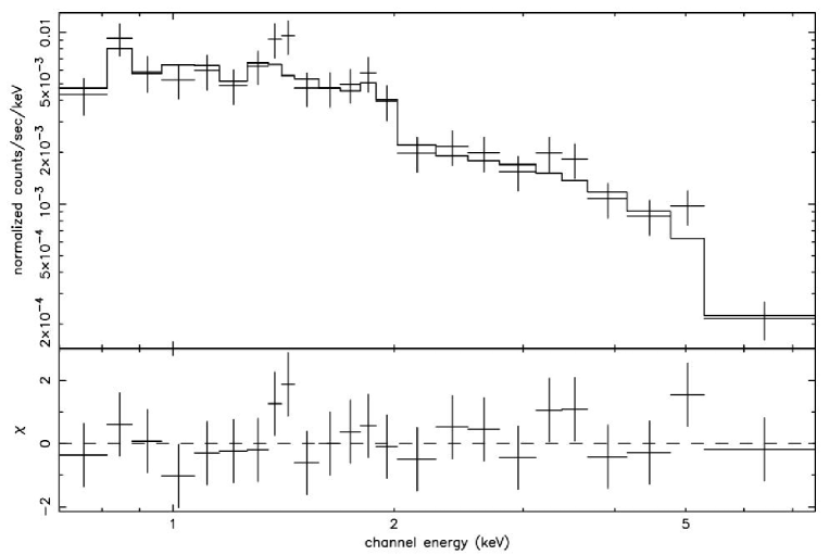
Figure 5: Energy spectrum of source #17, fit with an absorbed mekal model.

The spectrum of source #17 (Fig. 5) is even harder than that of source #4. It can be equally well fitted with a power-law model, with $\Gamma\approx 1.3$, and a mekal model, with $kT\sim 40$ keV and $L_{x}(0.5-8\,{\rm keV})\sim 5\times 10^{32}$ erg s^-1. The blackbody fit does not look acceptable, because of the high $\chi_{\nu}^{2}=1.73$ (the model underestimates the number of counts below 1 keV and above 5 keV) and unrealistically low $N_{22}<0.03$. The hardness of the spectrum is inconsistent with source #17 being a qLMXB, while its variability with a timescale of years (see §2.3) rules out a MSP interpretation. The luminosity of source #17 is lower than that of #4 so the argument against the CV interpretation is not so strong. On the other hand, source #17 is substantially closer to the cluster’s center, so the probability that it belongs to the cluster is higher. Therefore, a CV interpretation looks more plausible.

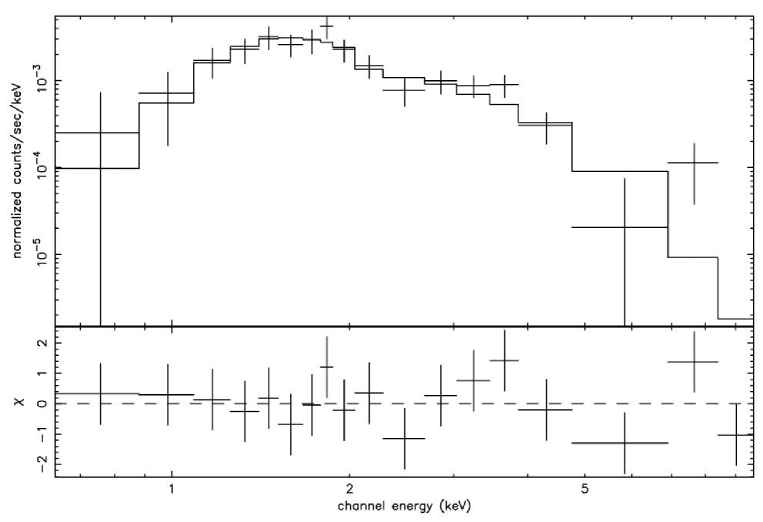
Figure 6: Energy spectrum of source #28, fit with an absorbed power-law model.

Source #28 shows a softer spectrum (Fig. 6), in comparison with sources #4 and #17, with possible absorption or an intrinsic turnover at softer energies. Because of the small number of counts detected, we cannot distinguish between different fits statistically. Both the power-law fit ($\Gamma\approx 3$, $N_{22}\sim 1.8$) and mekal ($kT\approx 2$ keV, $N_{22}\sim 1.4$) require an absorption column much higher than expected for a Galactic source in this direction. On the other hand, the blackbody fit yields a lower (albeit rather uncertain) absorption, $N_{22}\sim 0.3-1.1$. The blackbody temperature, $kT_{\rm BB}\sim 0.7$ keV, and the radius, $R_{\rm BB}\sim 100$ m, indicate that it might be thermal emission from an MSP polar cap. As we have discussed for source #4, a light-element atmosphere model would give a lower temperature, $kT\sim 0.3$ keV, and a larger radius, $R\sim 1$ km, which makes the MSP interpretation even more plausible. The observed spectrum of source #28 is harder than observed from qLMXBs, so we consider the qLMXB interpretation unlikely.

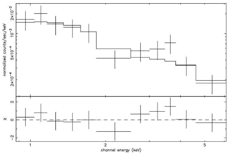
Figure 7: Energy spectrum of source #25, fit with an absorbed power-law model.

Finally, the hard spectrum of source #25 (Fig. 7) strongly resembles that of source #17, although with much fewer counts. The blackbody model is unacceptable, while both the power-law and mekal yield reasonable fits. Similar to source #17, we consider source #25 as a plausible CV candidate.

2.2.4 X-ray color-luminosity relation

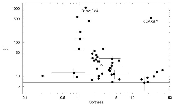
Figure 8: X-ray luminosity (0.5–8.0 keV), in units of $10^{30}$ erg s^-1, vs. X-ray color for the sources listed in Table 3. The X-ray color (softness) is here defined as the rate in the 0.2–2.0 keV band divided by the rate in the 2.0–8.0 keV band. The open circle marks the softness for the average spectrum of the 40 faintest sources at their average luminosity of $2.25\times 10^{31}$ erg s^-1. Error bars are displayed for selected sources. For the dimmest sources, X-ray color is, practically speaking, unknown. The PSR B1821$-$24 is the most luminous source in our sample. The source at the top right of the diagram, #26, is possibly a qLMXB.

Figure 8 shows a plot of X-ray luminosity versus an X-ray “color”. Such X-ray “color-magnitude diagrams” (CMDs; see Grindlay et al. 2001) are particularly useful for studying source populations in clusters where a large dynamic range of source luminosities and types can be studied at a common distance. The source with the highest luminosity, and hardest spectrum, is the PSR B1821$-$24. The source with the second highest luminosity we consider to be a good candidate for a quiescent low-mass X-ray binary (qLMXB) based on its spectral properties discussed in § 2.2.3. The other sources presumably are a mix of CVs (especially those with luminosities $\gtrsim 10^{32}$ erg/s), RS CVns, main-sequence binaries, MSPs, and other (unknown) systems.

Allowing for error bars on derived source colors and luminosities, it is clear that the CMD is most useful for the classification of brighter sources. However, even for faint sources, with poor statistics on each, a sufficiently large number of objects in the CMD can define an approximate distribution of source types (e.g. the MSPs in 47 Tuc) and constrain the possible source types of unidentified sources. In this observation, this has not been the case once the uncertainties are accounted for. Nevertheless, it is interesting to speculate that many of the soft, faint sources are lower luminosity MSPs as in 47 Tuc.

2.2.5 Spectroscopy of the central unresolved emission

As discussed in § 2.1, unresolved X-ray emission is present in the CXO data. This emission extends to roughly one core radius from the center of M28. If we take the total counts detected within $15^{\prime\prime}$ and subtract off the known contribution from point sources (including the estimated counts from the full PSF) then we are left with an excess of about 541 counts. To extract this spectrum, counts near the point sources were removed. The resulting spectrum contained 568 counts in good agreement with our estimate for the excess. The background contribution to this total is $\sim$100 counts. The spectrum was modeled using both a power-law model and a compound model consisting of a power-law with an additional optically-thin thermal emission-line (mekal) model. To account for the underabundance with respect to solar expected in the globular cluster, the abundance of metals in the mekal model were set to 2% of their solar values. The best-fitting model is the compound model ($\chi^{2}=30.4$ for 32 dof) though the mekal component is significant at only the $\sim 2\sigma$ level ($\chi^{2}=37.3$ for 34 dof for the power-law-only model). The best-fit photon index is $\Gamma=1.79^{+0.37}_{-0.32}$, and the temperature of the emission-line component is $kT=0.18^{+0.11}_{-0.07}$ keV. The luminosity is $2.9^{+0.3}_{-0.3}\times 10^{32}$ ergs s^-1 ($6.0^{+1.1}_{-1.8}\times 10^{32}$ ergs s^-1 after correction for absorption).

Interestingly, the photon index is similar (but not identical) to that deduced from co-adding the 40 weakest resolved sources (§2.2). This suggests a portion of the unresolved emission may be from point sources below the detection threshold but with similar spectral properties as those above the detection threshold.

We find that the X-ray $\log N(>S)$-$\log S$ distribution of the 12 sources within 15$\arcsec$ of the cluster center is $N(>S)\sim 52\,S^{-0.53}$. Assuming that this relationship extends to lower counting rates, we can estimate the number of photons that could come from sources below our threshold of  10 counts. This extrapolation predicts that $\sim 200$ counts or $\sim 1.2\times 10^{32}$ ergs s^-1 is contributed by sources below the detection threshold. Thus, unresolved sources with spectral properties similar to the weaker resolved sources can account for roughly half the observed power-law component of the unresolved emission.

We know that there are at least 4 distinct populations that could account for the unresolved emission: CVs, MSPs, BY Dra and RS CVn binaries, and isolated stellar coronae. If we assume that the unresolved emission, about $3\times 10^{32}$ ergs s^-1(unabsorbed), is entirely due to stellar coronae and there are about $10^{5}$ stars in the volume that gives rise to the unresolved emission, then this implies that the average stellar corona radiates at $\sim 3\times 10^{27}$ ergs s^-1. Since our Sun’s X-ray luminosity varies between $3\times 10^{26}$ and $5\times 10^{27}$ ergs s^-1 (Peres et al. 2000), we can say with confidence that the average star in M28 is less active than our Sun at its peak. This is not unexpected, since X-ray activity appears to correlate with rotation, and the old stars in M28 are likely slowly rotating. Therefore, we appeal to the usual suspects, faint CVs, MSPs, and RS CVn and BR Dra binaries, to account for the excess background emission. The X-ray luminosity functions for these classes are of course uncertain at the faint end. Assuming average luminosities in the range $1\times 10^{29}$ to $2\times 10^{30}$ ergs s^-1implies 50–1000 such sources.

2.3 Time Variability

We have used the three available ACIS observations to search for source variability on a time scale of weeks. The separate images are shown in Figure 9, while Figure 10 shows the variation in the counting rates. For all of the 46 sources, the number of counts detected in each of the 3 observations was computed by modeling the spatial distribution of events with a two-dimensional circular gaussian function with a width increasing according to the off-axis angle to approximately match the point spread function. Contributions from nearby sources were accounted for by using the same gaussian function out to a distance of 7 $\sigma$ from the source considered. In each case, both the position and width of the gaussians were kept constant in the data fitting, with only the normalizations left as free parameters. This approach gives a reasonable estimate for the number of counts from each source, even if the source was below the detection threshold and/or confused with another nearby source. As a check, the merged data was also examined and the results compared to the sums obtained from the 3 separate data sets. The observed counting rates agreed to better than 1.5%, indicating no obvious biases in our procedure.

For each source, we then calculated the deviations of the number of counts measured in each observation with respect to a constant flux distribution. By adding the 138 measurements ($46\times 3$), this calculation yielded a $\chi^{2}$ of 379.7 for 92 dof, clearly showing that some of the sources actually varied. The second observation of source #10 contributed the most (44.7) to $\chi^{2}$, and so we designated that source as “variable”. The three observations of this source were then removed from the sample. We then repeated this process. In this way we determined that 12 of the 46 sources exhibit evidence for some form of time variability. Setting aside these 12 sources, $\chi^{2}$ was 128.4 for 102 measurements and 68 degrees of freedom. The largest contribution now (#28, 2nd measurement) contributes only 5.95 to $\chi^{2}$ ($2.44\sigma$ deviation). Although it is likely that this source also varies (as do a few others) the level is low enough to make characterizing the variability difficult, and thus we did not ascribe any designation of variability to these sources.

To characterize the variability further, if a source in one observation is more than a factor of 2 above the average for the other two measurements, we say that it brightened (”b” in Table 3). Likewise, if one observation is more than a factor of 2 below the average for the other two measurements, we say that it dimmed (”d” in Table 3). If the source neither “brightened” nor “dimmed” according to these definitions, but was still identified as varying we denote it with a ”v”.

The source identified as a possible qLMXB (#26) was flagged as variable. Since the emission is dominated by a very slowly cooling black body (§2.2.2), variability is not expected. The variability designation is a consequence of the third observation being 13 percent ($4\sigma$) higher than the first two. There are a number of possible systematic effects that might produce such an effect. We verified the integration time for all three observations by counting the number of ACIS frames. We also searched for missed bad pixels and columns by checking which physical pixels were included in the extraction region, and found none. Furthermore, the small change in the spacecraft roll (12 degrees) between observations combined with the spacecraft dither, resulted in a common set of pixels for all three measurements. It is worth noting that cosmic ray tracks, the effects of which are discarded by the ACIS flight software, can produce up to 10 percent variations in sensitivity, but of the front-illuminated (FI) chips. Our observations, however, were performed with a back-illuminated CCD. These are much thinner than the FI chips and consequently these tracks are about 10 times smaller, with a corresponding smaller impact on sensitivity. In summary, we were unable to find any instrumental effect that could account for the observed variability for source #26. On the other hand, the small amplitude of the variability suggests caution in applying the designation.

In addition to the millisecond pulsar, we were also able to compare counting rates with one other ROSAT observation — that of the source with the fourth largest number of detected counts, #17. This source is located outside of the core radius at $42^{\prime\prime}$ from the cluster’s optical center. Although this source appears constant during our CXO observations, ROSAT observations indicate that the source is variable on time scales of years. Specifically, this source was not detected in either the ROSAT PSPC observation of March 1991 nor the ROSAT HRI observation of September 1995. The source was, however, detected with ROSAT HRI in September 1996.

To summarize, in the CXO data we found 6 sources that brightened, 3 that were variable, and 2 that dimmed. In addition, we found one variable source from the ROSAT data. Seven of these 13 sources are within one core radius of the center of the globular cluster. Of these seven, the three that brightened are most probably main sequence stars, whereas the two that were designated variable and the two that dimmed are most likely CVs (or perhaps qLMXBs). Finally, all the sources that appear to vary on shorter time scales (within one of the observations) had already been identified as varying by the technique described above.

3 Optical observations

We have performed a search for potential optical counterparts of the X-ray sources listed in Table  3 using data obtained with the HST WFPC2 and available in the public HST data archive. The observations of the M28 field were taken with the “V-band” filter F555W ($\lambda=5500$ Å; $\Delta\lambda=1200$Å) and the “I-band” filter F814W ($\lambda=7995$ Å; $\Delta\lambda=1292$ Å) on 1997 September 12 (Testa et al. 2001). To allow for a better cosmic ray filtering, the observations were split into a sequence of eight 140 s exposures in the F555W filter, and three 180 s plus six 160 s exposures in the F814W filter. Three short exposures of 2.6 s each were acquired in both filters to obtain unsaturated images of bright cluster stars. The total integration time was 1130 s and 1510 s in the F555W and F814W filters, respectively. The same data have been used by Golden et al. (2001) to search for the optical counterpart of the MSP B1821-24.

Data reduction and photometric calibration were performed through the HST WFPC2 pipeline. For each filter, single exposures were combined using a cosmic ray filter algorithm. The final images were then registered on each other. Automatic object extraction and photometry was run by using the ROMAFOT package (Buonanno and Iannicola 1989). The source lists derived for each passband were finally matched to produce the color catalog. Conversion from pixel to sky coordinates was computed using the task metric which also applies the correction for the WFPC2 geometrical distortions (see Testa et al. 2001 for further details on the data reduction and analysis).

The final catalog, consisting of a total of 33972 entries, with coordinates and magnitudes in the F555W passband and the F555W-F814W color, has been used as a reference for the optical identification. As a first step, the optical catalog has been cross-correlated with our list of X-ray sources. Since the ACIS astrometry has been boresighted using the pulsar’s radio coordinates as a reference (§2.1), the cross-correlation radius accounts only for the statistical error of the X-ray position and for the uncertainty of the HST astrometry. The latter is ascribed to the intrinsic error on the absolute coordinates of the GSC1.1 guide stars used to point the HST and compute the astrometric solution. Typical uncertainties are of the order of 1$\farcs$0 (see, e.g. Biretta et al.  2002)

Twenty-two of the X-ray sources were in the HST field-of-view, and each of them has potential WFPC2 counterparts. Figure 11 shows the location of all the 376 matched WFPC2 sources on the color-magnitude diagram (CMD) derived from all the sources detected in the WFPC2 field of view. The measured magnitudes have been corrected for the interstellar reddening assuming the same color excess E$(B-V)=0.43$ (Harris et al. 1996) for all the sources. Most of the candidate counterparts lie on the globular cluster main sequence, with only a few of them possibly associated with evolved stellar populations. We note that using any other average value of the reddening [e.g., E$(V-I)=0.52$, derived directly from our datasets], merely shifts the whole CMD. However, a more accurate analysis of the stellar populations may require accounting for possible differential reddening along the line of sight (Testa et al. 2001). This could narrow the distribution.

Additional F555W (340 s) and F814W (340 s) WFPC2 observations of the M28 field, taken on 1997 August 8, have been used to search for variability among the potential WFPC2 counterparts. The data have been retrieved from the ST-ECF public archive after on-the-fly recalibration with the best available reference files. The two pointings are centered very close to each other but with a slight relative rotation angle ($\sim\mathrm{5}^{\circ}$ ). Image co-addition, object detection and position measurements were performed consistent with the previous analyses. To avoid systematic effects due to the difference in the default astrometric solution between the two datasets, which has been measured to be of the order of 1$\farcs$0, the object catalogs derived from the August 8 and September 12 observations were matched in the pixel space after registering the two sets of coordinates through a linear transformation. The overall dispersion of the radial coordinate residuals after the transformation turned out to be 0.17 WFC pixels (0$\farcs$017). For this reason, only objects with radial coordinate residuals smaller than 0.5 WFC pixels, i.e. 3 $\sigma$ of the dispersion of the residuals, were considered as matched in the two datasets and examined for variability. Possible spurious matches were checked manually and filtered out.

Although a number of candidates show brightness variation larger than 0.5 magnitudes in at least one of the filters, their nature cannot be assessed with high confidence. Some of them are indeed close to the detection limit, hence with larger photometry errors, while others are detected too close to bright stars to obtain clean measurements even using PSF subtraction alghoritms, and a few are located in very crowded patches.

We note that some objects detected in the first dataset are absent in the second. All these cases have been checked carefully to find out whether the lack of matches was due to intrinsic object variability. However, we found that the missing matches can be explained either by the fact that in the second dataset some objects fall at the chip edge or in the overscan region, or they fall out of the field of view or, as the second dataset is shallower, they are simply below the detection limit.

Although we have found a number of candidate counterparts to the X-ray sources, no definite conclusions can yet be drawn from our search. In the crowded globular cluster field, the dominant uncertainty in the HST astrometry represents the real bottleneck for obtaining optical identifications. In contrast, e.g., to the experience of Pooley et al.  (2002a) with NGC 6752, we found very few blue candidates which can be considered as likely counterparts and used to boresight the HST astrometry. At the same time, no GSC2.1 or USNO-A2.0 stars are present in the narrow WFPC2 field of view to use them as a reference to recompute the image astrometric calibration. The only way to improve the WFPC2 astrometry of our datasets is by upgrading the coordinates and the positional accuracy of the guide stars used for the telescope pointing and recomputing the astrometric solution in the HST focal plane. This, together with a larger spectral coverage, will definitely give us a better chance to obtain firm identifications.

4 Summary

We have analyzed observations of the globular cluster M28 taken with the ACIS-S3 instrument aboard the CXO. Forty-six X-ray sources were detected within $3\farcm 1$ of the optical center of the cluster down to a limiting (absorption-corrected) luminosity of $\sim 6.8\times 10^{30}$ ergs s^-1 in the 0.5 – 8.0 keV range. Many of these sources are concentrated near the center of the cluster. Their radial distribution can be described by a King profile with an X-ray core radius comparable to that of optical light but with a steep power-law index suggesting a rather high X-ray source population mass, $M_{x}\sim 1.9$ M_⊙. The X-ray source distribution flattens at larger radii consistent with a population of background sources.

Among the brightest sources in M28 is the millisecond pulsar PSR B1821$-$24. We find the phase-averaged spectrum of PSR B1821$-$24 to be best represented by a $\Gamma=1.20$ power law radiating at $L_{x}=1.3\times 10^{33}$ ergs s^-1. The luminosity is consistent with a steady luminosity since the time of ROSAT observations.

An intriguing spectral feature, albeit of marginal statistical significance, observed at $\sim$3 keV in PSR B1821$-$24 might be an electron cyclotron line. If so, the line requires a magnetic field of order 100 times the strength inferred from $P$ and $\dot{{P}}$ suggesting the local magnetic field at the surface of the neutron star is well above the conventional values obtained by assuming a centered dipole geometry. This may be due to multipolar components, to a strong off-centering of the magnetic dipole, or to a combination of the two. Recently, Gil & Melikidze (2002) argued on both observational and theoretical grounds that such strong deviations from the dipole magnetic field should exist at or near pulsar polar caps. Geppert & Rheinhardt (2002) showed that it is possible to create strong but small-scale poloidal field structures at the neutron star surface via a Hall-instability from subsurface toroidal field components.

A second bright source, closer to the center of M28, was also studied in detail. The spectrum of this source (#26) is notably soft and thermal (Fig. 3) as is typical of transiently-accreting neutron stars in quiescence. Such objects have a hydrogen-rich atmosphere comprised of matter accumulated and heated during previous accretion episodes. Non-magnetic hydrogen atmosphere models provide the best fit to the spectrum of this source and thereby support this interpretation. The bolometric luminosity corresponding to the best fit model parameters, $L_{\rm bol}^{\infty}\sim 1.9\times 10^{33}$ ergs s^-1, can be maintained by a time-averaged accretion rate of $\sim 2\times 10^{-11}$ M_⊙ yr^-1. While the flux from this source varies among the 3 CXO observations, there is no evidence for spectral variability between our observations taken at roughly 1 month intervals.

While CXO resolves many of the X-ray sources in M28, there remains some diffuse emission distributed over $\sim$1 core radius. This emission is only 22% of the total X-ray luminosity in the central region. Nevertheless, simple extrapolation of the observed $\log N$ – $\log S$ relation to below our detection threshold cannot account for more than about one-half of the emission. Another population of weak sources must account for the remainder. Possibilities include BY Dra and (weak) RS CVn systems, other millisecond pulsars, isolated low-mass stars, and CVs.

By scheduling our 3 observations of M28 over an $\sim$2 month period, we were able to observe variability in the resolved X-ray source population on a time scale of order weeks. Twelve of the sources, or 26%, are seen to vary over the course of the observations including the quiescent low-mass X-ray binary. Some sources exhibited a much higher flux in 1 of the 3 observations, and may be associated with stellar coronae. Others display the opposite effect, being low in one observation or otherwise varied and may be associated with CVs and qLMXBs.

Finally, the benefit of an accurate radio position for PSR B1821$-$24 has allowed us to constrain the X-ray positions of the M28 sources to sub-pixel accuracy. Comparison to HST images suffers, however, from the intrinsic error in the absolute coordinates of the GSC1.1 guide stars used to compute the WFPC2 astrometric solution thus preventing any conclusive identifications.

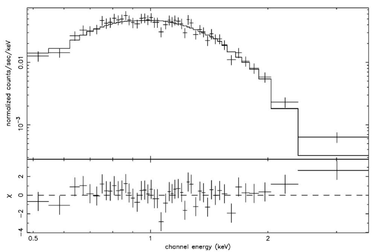
Figure 3: Energy spectrum of source #26. The spectrum is modeled with a nonmagnetic neutron star H atmosphere model.

Figure 9: ACIS-S3 image of the central region of M28 at three separate epochs (A, B, C) as per Table 1.

Figure 10: The count rate for all sources for each of the three observations. The x-axis is the row number listed in Table 3. For each source, three rates are plotted: a circle for the first observation, an “x” for the second, and a triangle for the third. Any missing points were below the minimum rate plotted. The statistical error bar is also plotted, but for the high count rate sources it is difficult to see. The variability indicators (b, v and d) are discussed in § 2.3.

Figure 11: Color-magnitude diagram for all the sources detected in the WFPC2 field of view (light grey points). The magnitudes are corrected for the interstellar extinction using the same E$(B-V)=0.43$ for all the sources. The 376 HST candidate counterparts matched to the X-ray sources listed in Table 3 are indicated by grey filled circles.

Table 1: CXO Observations

Date	ObsID	Exposure
2002  July 4	2684	12.7 ksec
2002  Aug 8	2685	13.5 ksec
2002  Sep 9	2683	11.4 ksec

Table 2: PSR B1821$-$24 Positions (J2000)

Date	Position
2002 July 4	18 24 32.015	$-$24 52 10.81
2002 Aug 8	18 24 32.016	$-$24 52 10.76
2002 Sep 9	18 24 32.009	$-$24 52 10.83
average	18 24 32.013	$-$24 52 10.80
rms (arcsec)	0.042	0.029
merged data	18 24 32.013	$-$24 52 10.80
radio (8/02)	18 24 32.008	$-$24 52 10.76

Table 3: M28 Discrete X-Ray Sources

	R.A.	Dec.	$r^{a}$	$d^{b}$	S/N	Softc	Mediumd	Harde	$L_{X}{{}^{f}}$	Variabilityg
	(J2000)	(J2000)	($\arcsec$)	($\arcsec$)		($10^{-5}$ s-1)	($10^{-5}$ s-1)	($10^{-5}$ s-1)	($10^{30}$ erg s-1)
1	18 24 20.531	-24 51 33.04	0.433	172	4.09	$15.7_{-7.7}^{+7.0}$	$26.1_{-9.2}^{+8.6}$	$19.1_{-8.2}^{+7.6}$	$17.0$
2	18 24 20.619	-24 51 27.17	0.431	172	4.16	$15.8_{-7.8}^{+7.1}$	$35.3_{-10.6}^{+10.0}$	$13.3_{-7.2}^{+6.5}$	$17.8$	b
3	18 24 22.575	-24 52 05.69	0.361	140	5.02	$35.5_{-10.8}^{+10.2}$	$36.3_{-10.8}^{+10.2}$	$17.3_{-7.9}^{+7.2}$	$25.1$
4	18 24 22.684	-24 51 02.65	0.303	154	21.12	$47.9_{-12.2}^{+11.7}$	$663.4_{-43.3}^{+42.8}$	$756.5_{-46.3}^{+45.8}$	$578.9$	v
5	18 24 22.831	-24 52 46.06	0.469	141	2.60	$13.2_{-6.8}^{+6.2}$	$8.2_{-10.6}^{+4.8}$	$2._{-2.0}^{+8.7}$	$6.5$
6	18 24 24.237	-24 51 04.14	0.421	135	3.75	$14.9_{-8.2}^{+7.4}$	$36.8_{-11.6}^{+10.9}$	$1.7_{-1.7}^{+8.8}$	$15.3$
7	18 24 24.603	-24 53 02.10	0.392	123	3.14	$20.1_{-9.1}^{+8.3}$	$17.3_{-8.5}^{+7.6}$	$2.7_{-2.7}^{+11.1}$	$9.9$
8	18 24 25.175	-24 54 06.67	0.327	155	5.75	$54.8_{-14.1}^{+13.4}$	$55.5_{-14.1}^{+13.4}$	$27.1_{-10.3}^{+9.5}$	$33.4$
9 *	18 24 25.189	-24 52 13.60	0.408	104	2.82	$0_{-0.0}^{+4.2}$	$0_{-0.0}^{+4.2}$	$36.5_{-12.2}^{+11.4}$	$9.3$
10	18 24 25.658	-24 50 34.14	0.407	138	4.58	$21.3_{-8.6}^{+7.9}$	$31.3_{-9.9}^{+9.3}$	$12.9_{-7.0}^{+6.3}$	$20.4$	b
11	18 24 28.449	-24 50 33.59	0.423	114	3.72	$11.4_{-7.4}^{+6.5}$	$32.9_{-10.9}^{+10.2}$	$11.8_{-7.4}^{+6.5}$	$14.6$
12 *	18 24 28.580	-24 53 09.77	0.359	82	3.11	$0_{-0.0}^{+3.2}$	$17.1_{-7.5}^{+6.8}$	$16.9_{-7.5}^{+6.8}$	$9.7$
13 *	18 24 28.727	-24 51 24.56	0.405	73	3.23	$10._{-6.1}^{+5.3}$	$13.4_{-6.6}^{+6.0}$	$10.2_{-6.1}^{+5.3}$	$10.2$
14 *	18 24 30.155	-24 51 49.81	0.323	42	5.76	$18.9_{-8.5}^{+7.8}$	$68.7_{-15.1}^{+14.5}$	$48.7_{-12.9}^{+12.2}$	$34.8$
15 *	18 24 30.770	-24 52 33.19	0.367	36	2.91	$13.7_{-6.9}^{+6.2}$	$14.1_{-6.9}^{+6.2}$	$0_{-0.0}^{+3.2}$	$8.3$
16 *	18 24 30.946	-24 52 13.84	0.323	26	5.12	$23.3_{-8.8}^{+8.1}$	$53.5_{-12.8}^{+12.2}$	$32.3_{-10.1}^{+9.5}$	$27.5$
17 *	18 24 31.063	-24 52 45.20	0.299	41	18.77	$254.3_{-26.3}^{+25.8}$	$537.6_{-38.1}^{+37.6}$	$514.9_{-37.3}^{+36.8}$	$439.1$	vh
18 *	18 24 31.591	-24 52 17.49	0.377	18	2.88	$5.3_{-5.3}^{+19.9}$	$14.5_{-7.0}^{+6.3}$	$11.3_{-6.5}^{+5.7}$	$7.8$
19 *	18 24 32.008	-24 52 10.76	0.298	11	30.09	$526.4_{-38.9}^{+38.4}$	$1369_{-63}^{+62}$	$1405_{-63}^{+63}$	$96.0$
20	18 24 32.213	-24 53 51.58	0.331	100	3.69	$21.5_{-8.0}^{+7.5}$	$24.5_{-8.5}^{+7.9}$	$13.4_{-6.6}^{+5.9}$	$15.6$
21 *	18 24 32.272	-24 52 09.46	0.323	8	4.85	$29.5_{-9.7}^{+9.1}$	$77.6_{-15.2}^{+14.7}$	$47.5_{-12.1}^{+11.5}$	$27.6$
22 *	18 24 32.345	-24 52 08.02	0.316	8	5.30	$35.4_{-10.6}^{+10.0}$	$116.4_{-18.5}^{+18.0}$	$68.4_{-14.4}^{+13.8}$	$37.2$	d
23 *	18 24 32.514	-24 52 07.66	0.312	6	6.73	$44.3_{-11.7}^{+11.2}$	$95.6_{-16.9}^{+16.3}$	$137.3_{-20.1}^{+19.6}$	$64.5$
24 *	18 24 32.631	-24 52 21.70	0.354	10	3.35	$13.7_{-6.9}^{+6.2}$	$22.7_{-8.4}^{+7.8}$	$13.8_{-6.9}^{+6.2}$	$12.0$	b
25 *	18 24 32.689	-24 52 23.54	0.304	12	9.65	$54._{-12.6}^{+12.1}$	$129.1_{-19.1}^{+18.6}$	$172._{-22.0}^{+21.5}$	$129.0$
26 *	18 24 32.821	-24 52 08.26	0.298	3	36.93	$2213.8_{-79.5}^{+79.}$	$2477.1_{-84.1}^{+83.6}$	$211.7_{-24.9}^{+24.3}$	$534.0$	v
27 *	18 24 33.026	-24 52 01.72	0.353	9	3.46	$8.7_{-11.3}^{+5.1}$	$12._{-6.7}^{+5.9}$	$24._{-8.9}^{+8.3}$	$12.7$	b
28	18 24 33.026	-24 50 52.86	0.306	78	13.72	$42.9_{-11.5}^{+10.9}$	$278._{-28.1}^{+27.6}$	$298.1_{-29.1}^{+28.6}$	$207.9$
29 *	18 24 33.070	-24 52 10.45	0.308	2	7.90	$67.6_{-14.3}^{+13.7}$	$124.4_{-19.1}^{+18.5}$	$67.8_{-14.3}^{+13.7}$	$65.8$	v
30 *	18 24 33.429	-24 52 15.49	0.313	8	6.50	$34.6_{-10.3}^{+9.8}$	$76._{-14.9}^{+14.4}$	$52.3_{-12.5}^{+12.0}$	$42.8$	b
31	18 24 33.539	-24 52 33.16	0.316	23	5.62	$13.6_{-6.8}^{+6.1}$	$61.9_{-13.3}^{+12.7}$	$36.3_{-10.3}^{+9.8}$	$31.5$
32 *	18 24 33.634	-24 52 12.12	0.312	10	6.74	$17.2_{-7.7}^{+7.0}$	$103.4_{-17.4}^{+16.9}$	$67.6_{-14.2}^{+13.7}$	$47.3$	d
33 *	18 24 33.759	-24 52 11.08	0.321	11	4.87	$38.1_{-10.9}^{+10.3}$	$71.1_{-14.6}^{+14.0}$	$20.4_{-8.2}^{+7.6}$	$29.4$
34 *	18 24 33.861	-24 51 11.99	0.391	60	3.59	$7.4_{-10.2}^{+4.6}$	$24.5_{-8.5}^{+8.0}$	$7.5_{-10.2}^{+4.6}$	$11.8$
35 *	18 24 34.469	-24 53 12.99	0.335	65	3.67	$26.9_{-8.8}^{+8.3}$	$21.7_{-8.0}^{+7.4}$	$0_{-0.0}^{+3.}$	$13.4$
36	18 24 34.974	-24 54 57.88	0.368	168	3.39	$18.5_{-8.3}^{+7.6}$	$28.7_{-10.}^{+9.3}$	$12.2_{-7.1}^{+6.2}$	$11.3$
37	18 24 35.524	-24 52 18.34	0.321	36	5.45	$14.3_{-7.1}^{+6.4}$	$53.3_{-12.7}^{+12.1}$	$35.2_{-10.5}^{+9.9}$	$29.5$
38	18 24 36.578	-24 50 16.04	0.340	125	7.58	$52.9_{-12.6}^{+12.1}$	$74.3_{-14.7}^{+14.2}$	$64.8_{-13.9}^{+13.3}$	$56.5$
39	18 24 37.326	-24 51 57.50	0.363	61	3.46	$25.9_{-9.8}^{+9.1}$	$16.4_{-8.0}^{+7.2}$	$2.7_{-2.7}^{+10.8}$	$13.2$
40	18 24 37.831	-24 51 44.58	0.401	72	2.93	$13.1_{-7.9}^{+6.9}$	$17.5_{-8.6}^{+7.7}$	$2.6_{-2.6}^{+11.1}$	$9.1$	b
41	18 24 37.897	-24 49 28.45	0.632	176	2.75	$2.5_{-2.5}^{+10.7}$	$19.4_{-8.1}^{+7.5}$	$9.1_{-6.4}^{+5.7}$	$8.6$
42	18 24 39.061	-24 51 08.26	0.434	105	3.15	$4.7_{-4.7}^{+18.}$	$2.5_{-2.5}^{+9.9}$	$29.1_{-9.8}^{+9.2}$	$10.3$
43	18 24 39.567	-24 50 30.18	0.561	136	2.63	$12.5_{-6.9}^{+6.3}$	$10.9_{-6.4}^{+5.6}$	$1.3_{-1.3}^{+7.3}$	$6.8$
44	18 24 40.336	-24 50 35.31	0.563	139	2.64	$12.5_{-7.}^{+6.3}$	$5.1_{-5.1}^{+19.4}$	$4.2_{-4.2}^{+16.3}$	$6.8$	b
45	18 24 41.303	-24 54 16.97	0.419	170	2.63	$0_{-0.0}^{+4.1}$	$25.4_{-10.2}^{+9.4}$	$2.7_{-2.7}^{+11.4}$	$8.1$
46	18 24 42.694	-24 52 47.48	0.433	138	2.81	$10.1_{-6.2}^{+5.4}$	$13.6_{-6.7}^{+6.0}$	$4.7_{-4.7}^{+18.2}$	$8.1$

Note. —

Sources indicated with a * are in the field of view of the HST observations discussed in § 3

^a Positional uncertainty radius in arcsec (see text).

^b Distance from the nominal optical center of the cluster.

^c Detected counting rate, corrected for the psf, in the 0.2–1.0 keV band.

^d Detected counting rate, corrected for the psf, in the 1.0–2.0 keV band.

^e Detected counting rate, corrected for the psf, in the 2.0–8.0 keV band.

^f X-ray luminosity in the 0.5–8.0 keV band assuming a distance of 5.5 kpc and $N_{H}$ of $0.18\times 10^{22}$ cm^-2. The luminosities of the six brightest sources are based on a canonical power-law. More accurate luminosities for the six brightest sources are presented in the text.

^g v indicates variability, f a flare and d a dip as discussed in § 2.3.

^h based on comparison with ROSAT observations.

Table 4: Extraction and spectral fitting parameters

source #	$r_{\rm ext}^{a}$	fb	$N_{S+B}^{c}$	$N_{B}^{d}$	$N_{\rm min}^{e}$	$N_{\rm bins}^{f}$
19	$1\farcs 72$	97.5	1119	2	30	34
26	$1\farcs 72$	97.5	1669	2	30	47
4	$8\farcs 9$	100	540	49	15	33
17	$7\farcs 5$	100	527	28	20	24
28	$14\farcs 8$	95	300	115	15	18
25	$1\farcs 35$	95	127	1	10	11

Note. —

^a Extraction radius

^b Approximate percentage of total signal

^c Total number of extracted counts.

^d Estimated number of background counts.

^e Minimum number of counts per spectral bin.

^f Number of spectral bins.

Table 5: Spectral Fit

source	modela	$\chi_{\nu}^{2}$	$\nu$	$N_{H}/10^{22}$	$\Gamma$ or $kT$b	Radiusc	$\mbox{Flux}^{d}/10^{-13}$
number				$\mbox{cm}^{-2}$		km	${\rm erg}\,{\rm cm}^{-2}\,{\rm s}^{-1}$
19 (PSR)	pl	0.89	31	$0.16^{+0.07}_{-0.08}$	$1.20^{+0.15}_{-0.13}$		$3.54^{+0.06}_{-0.05}$
26	bb	1.10	44	$0.13_{-0.05}^{+0.05}$	$0.26_{-0.18}^{+0.18}$	$1.27_{-0.23}^{+0.29}$	$1.59_{-0.71}^{+1.38}$
26	pl	0.86	44	$0.68_{-0.07}^{+0.08}$	$5.24^{+0.39}_{-0.35}$		$14.8_{-3.95}^{+0.65}$
26	nsa	0.96	44	$0.26_{-0.04}^{+0.04}$	$0.09^{+0.03}_{-0.01}$	$14.5_{-3.8}^{+6.9}$	$3.35_{-1.1}^{+1.9}$
26	mekal	0.88	44	$0.33_{-0.05}^{+0.02}$	$0.59^{+0.06}_{-0.06}$		$3.26_{-1.04}^{+1.60}$
4	bb	1.39	30	$0.16_{-0.13}^{+0.16}$	$1.07^{+0.13}_{-0.11}$	$0.063_{-0.01}^{+0.02}$	$1.69_{-0.95}^{+0.66}$
4	pl	1.14	30	$0.86_{-0.18}^{+0.26}$	$1.59^{+0.15}_{-0.24}$		$2.49_{-0.26}^{+0.71}$
4	mekal	1.14	30	$0.77_{-0.17}^{+0.19}$	$13.3^{+41.4}_{-6.7}$		$2.34_{-0.48}^{+0.14}$
17	bb	1.73	21	$0.0-0.028$	$0.88^{+0.08}_{-0.76}$	$0.073_{-0.01}^{+0.01}$	$1.07^{+0.89}_{-0.49}$
17	pl	1.02	21	$0.17^{+0.15}_{-0.1}$	$1.30^{+0.21}_{-0.18}$		$1.47^{+0.15}_{-0.11}$
17	mekal	0.99	21	$0.17^{+0.11}_{-0.17}$	$38^{+42}_{-26}$		$1.44^{+0.13}_{-0.19}$
28	bb	0.67	15	$0.64^{+0.52}_{-0.36}$	$0.67^{+0.14}_{-0.12}$	$0.095_{-0.03}^{+0.06}$	$0.59^{+2.76}_{-0.48}$
28	pl	0.74	15	$1.83^{+0.93}_{-0.63}$	$3.08^{+1.00}_{-0.67}$		$2.20^{+0.33}_{-0.44}$
28	mekal	0.68	15	$1.38^{+0.63}_{-0.47}$	$1.95^{+1.45}_{-0.72}$		$1.09^{+0.50}_{-0.37}$
25	bb	1.43	8	$0.0-0.13$	$1.12^{+0.27}_{-0.21}$	$0.026_{-0.66}^{+0.81}$	$0.340^{+0.91}_{-0.25}$
25	pl	0.77	8	$0.0-0.3$	$0.82^{+0.43}_{-0.33}$		$0.425^{+0.35}_{-0.02}$
25	mekal	1.11	8	$0.17^{+0.31}_{-0.17}$	$14.2-79.80$		$0.376^{+0.60}_{-0.03}$

Note. —

^a bb = blackbody; pl = power law; nsa = neutron star H-atmosphere; mekal = optically-thin thermal plasma.

^b The entry in this column depends on the spectral model — it is the power law index $\Gamma$ or the temperature $kT$ in keV ($kT_{\rm eff}^{\infty}$ for the nsa model).

^c Blackbody radius ($R_{\rm NS}^{\infty}$ for the nsa model).

^d Unabsorbed flux in the 0.5–8.0 keV band.

References

- (1) Becker, W., Aschenbach, B., 2002, in Proceedings of the WE-Heraeus Seminar on Neutron Stars, Pulsars and Supernova remnants, eds W.Becker, H.Lesch & J/Trümper, MPE-Report 278, 64, (available from astro-ph/0208466)
- (2) Becker, W., Pavlov, G.G., 2001, in The Century of Space Science, eds. J.Bleeker, J.Geiss & M.Huber, Kluwer Academic Publishers, p721 (available from astro-ph/0208356).
- (3) Becker, W. & Trümper, J. 1999, A&A, 341, 803
- (4) Biretta, J.A. et al. 2002, WFPC2 Instrument Handbook, Version 7.0 (Baltimore, STScI)
- (5) Brown, E. F., Bildsten, L., & Rutledge, R. E. 1998, ApJ, 504, L95
- (6) Cognard, I., Bourgois, G., Lestrade, J. F., Biraud, F., Aubry, D., Darchy, B., Drouhin, J. P. 1996, A&A, 311, 179
- (7) Cool, A.M., Grindlay, J.E., Krockenberger, M., & Bailyn, C.D., 1993, ApJ, 410, L103
- (8) Danner, R., Kulkarni, S.R., Saito, Y., & Kawal, N. 1997, Nat, 388, 751
- (9) Davidge, T. J, Cote, P., & Harris, W. E. 1996, ApJ, 468, 641
- (10) Davis, J.E. 2001, ApJ, 562, 575
- (11) Dickey, J. M., & Lockman, F. J. 1990, ARAA, 28, 215
- (12) Foster, R.S., Backer, D.C., Taylor, J.H., & Goss, W.M., 1988, ApJ, 326, L13
- (13) Freeman, P.E., Kashyap, V., Rosner, R., Lamb, D.Q. 2002. ApJS, 138, 185
- (14) Geppert, U., Rheinhardt, M., 2002, A & A, 392, 1015
- (15) Gil, J., Melikidze, G.I., 2002, ApJ, 577, 909
- (16) Golden A., Butler R.F., Shearer A., 2001, A& A 371, 198.
- (17) Gotthelf, E.V., & Kulkarni, S.R., 1997, ApJ, 490, L161
- (18) Grindlay, J. E., Heinke, C. O., Edmonds, P. D., Murray, S. S., Cool, A. M.2001, ApJ, 563, 53
- (19) Grindlay, J.E., Heinke, C., Edmonds, P.D., & Murray, S.S., 2001a, Science, 290, 2292
- (20) Grindlay, J.E., Camilo, F., Heinke, C.O., Edmonds, P.D., Cohn, H. & Lugger, P., 2002, ApJ, in press.
- (21) Harris, W. E., 1996, AJ, 112, 1487 (June 22, 1999 Version).
- (22) Hertz, P.& Grindlay, J.E, 1983, ApJ, 275, 105
- (23) Johnston, H.M., & Verbunt, F., 1996, A&A, 312, 80
- (24) Kawai N., Saito Y., 1999, Proc. 3rd INTEGRAL Workshop, Taormina, Astroph. Lett. & Comm. 38, 1
- (25) Lyne, A.G., Brinklow, A., Middleditch, J., Kulkarni, S.R., & Backer, D.C. 1987, Nature, 328, 399
- (26) Pavlov, G. G., Shibanov, Y. A., & Zavlin, V. E. 1991, MNRAS, 253, 193
- (27) Peres, G. Orlando, S., Reale, F, Rosner & Hudson, H, 2000, ApJ, 528, 537.
- (28) Phinney, E. S. 1993, ”Pulsars as Probes of Globular Cluster Dynamics”, ASP Conf. Ser. 50: ”Structure and Dynamics of Globular Clusters, 141
- (29) Pooley, D., Lewin, W. H. G., Homer, L., Verbunt, F., Anderson, S. F., Gaensler, B. M., Margon, B., Miller, J. M., Fox, D. W., Kaspi, V. M., & van der Klis, M. 2002a, ApJ, 569, 405
- (30) Pooley, D., Lewin, W., Verbunt, F., Homer, L., Margon, B., Gaensler, B., Kaspi, V., Miller, J.M., Fox, D.W., & van der Klis, M., 2002b, ApJ, 573, 184
- (31) Rasio, F.A., Pfahl, E.D. & Rappaport, S., 2000, ApJ, 532, 47
- (32) Rajagopal, M., & Romani, R. W. 1996, ApJ, 461, 327
- (33) Rees, R. F. & Cudworth, K. M. 1991, AJ, 102, 152
- (34) Rots, A.H., et al. 1998, ApJ, 501, 749
- (35) Rosati, P. et al. 2002, ApJ, 566, 667
- (36) Rutledge, R. E., Bildsten, L., Brown, E. F., Pavlov, G. G., & Zavlin, V. E. 2000, ApJ, 529, 985
- (37) Rutledge, R.E., Bildsten, L., Brown, E.F., Pavlov, G.C., & Zavlin, V.E. 2002a, ApJ, 578, 405
- (38) Rutledge, R. E., Bildsten, L., Brown, E. F., Pavlov, G. G., & Zavlin, V. E. 2002b, ApJ, 577, 346
- (39) Rutledge, R. E., Kulkarni, S. R., Fox, D. R., Jacoby, B. A., Cognard, I., Backer, D. C., & Murray, S. S. 2003, submitted to ApJ (astro-ph/0301453)
- (40) Saito, Y., Kawai, N., Kamae, T., Shibata, S., Dotani, T., & Kulkarni, S.R. 1997, ApJL, 477, L37
- (41) Salaris, M., Weiss, A., 2002, A&A 388, 492
- (42) Shawl, S.J. & White, R. E. 1986, AJ, 91, 312
- (43) Stetson, P.B. 1987, PASP, 99, 191
- (44) Swartz, D. A., Ghosh, K.K., McCollough, M.L., Pannuti, T.G., Tennant, A.F. & Wu, K. 2003, ApJS, 144, 213
- (45) Testa, V., Corsi, C. E., Andreuzzi, G., Iannicola, G., Marconi, G., Piersimoni, A. M. & Buonanno, R. 2001, AJ, 121, 916
- (46) Verbunt, F. 2001, A&A, 368, 137
- (47) Verbunt, F. & Hut, P. 1987, IAU Symp. 125, 187
- (48) Verbunt, F. 2002, “Binary Evolution and Neutron stars in Globular Clusters”,to appear in ASP Conference Series ”New Horizons in Globular Cluster Astronomy”, Eds. G. Piotto, G.Meyla,, G. Djorgvoski, & M. Riello.
- (49) Warren, B. 1995, Cataclysmic Variable Stars (Cambridge Univ. Press: Cambridge)
- (50) Wilms,J., Allen,A. & McCray,R. 2000, ApJ, 542, 914
- (51) Zavlin, V.E., Pavlov, G.G., & Shibanov, Y.A., 1996, A&A, 315, 141
- (52) Zavlin, V. E., & Pavlov, G. G. 1998, A&A, 329, 583