Ionized Gas in the First 10 kpc of the Interstellar Galactic Halo

Abstract

We present Far Ultraviolet Spectroscopic Explorer (FUSE) observations of the post-asymptotic giant branch star von Zeipel 1128 ($l=42\fdg 5,\,b=+78\fdg 7;\ d=10.2\ {\rm kpc},z=10.0\ {\rm kpc};\ v_{\rm LSR}=-140\pm 8$ km s^-1), located in the globular cluster Messier 3. The FUSE observations cover the wavelength range 905 – 1187 Å at $\sim 20$ km s^-1 (FWHM) resolution. These data exhibit many photospheric and interstellar absorption lines, including absorption from ions associated with the warm neutral, warm ionized, and highly-ionized phases of the interstellar medium along this sight line. We derive interstellar column densities of H I, P II, Ar I, Fe II, Fe III, S III, and O VI, with lower limits for C II, C III, N I, O I, and Si II. Though the individual velocity components within the absorption profiles are unresolved by FUSE, a comparison of the velocity distribution of depleted or ionized species with the neutral species suggests the thick disk material along this sight line is infalling onto the Galactic plane, while material near the plane is seen closer to rest velocities. Ionized hydrogen represents $\gtrsim 12\%$, most likely $\sim 45\%$, of the total hydrogen column along this sight line, most of it associated with the warm ionized phase. The warm ionized and neutral media toward von Zeipel 1128 have very similar gas-phase abundances and kinematics: the neutral and ionized gases in this region of the thick disk are closely related. Strong O VI absorption is seen with the same central velocity as the warm ionized gas, though the O VI velocity dispersion is much higher ($\sigma\equiv\sqrt{2}b=32$ km s^-1). Virtually all of the O VI is found at velocities where lower-ionization gas is seen, suggesting the O VI and WNM/WIM probes are tracing different portions of the same structures (e.g., the O VI may reside in interfaces surrounding the WNM/WIM clouds). We see no evidence for interstellar absorption associated with the globular cluster Messier 3 itself nor with the circumstellar environment of von Zeipel 1128. Neither high velocity cloud absorption (with $|v_{\rm LSR}|\gtrsim 125$ km s^-1) nor high velocity-dispersion gas (with $\sigma\sim 60$ km s^-1) is seen toward von Zeipel 1128.

1 Introduction

There is now substantial evidence that the interstellar medium (ISM) of the Milky Way is best described as a “multiphase” medium. In standard equilibrium models of the ISM (e.g., McKee & Ostriker 1977, Wolfire et al. 1995), the term “phase” refers to gaseous regions of distinct temperatures, densities, and ionization states. Most models assume these regions are physically independent and exist in (sometimes rough) pressure equilibrium. Extraplanar material in spiral galaxies seems to exhibit all of the principal phases found in the disk of the Milky Way: the cold neutral medium [CNM; $T\sim 10^{2}$ K; $x(\mbox{H$\;${\small\rm II}})\equiv n(\mbox{H$\;${\small\rm II}})/n({\rm H_{tot}})\sim 10^{-4}$; Howk & Savage 1999a, 2000; Richter 2001]; the warm neutral medium [WNM; $T\sim 10^{4}$ K; $x(\mbox{H$\;${\small\rm II}})\sim 0.1$; Dickey & Lockman 1990]; the warm ionized medium [WIM; $x(\mbox{H$\;${\small\rm II}})\gtrsim 0.8$; Reynolds 1993]; and the hot ISM [$T\sim 10^{6}$ K; $x(\mbox{H$\;${\small\rm II}})\sim 1.0$; Snowden et al. 1998].

While the evidence strongly suggests their presence in the extraplanar regions of the Milky Way, the properties and physics of these phases and their relationships are as yet poorly characterized for extraplanar gas. As such, there are many unanswered questions regarding the nature of gas in the thick disk of the Milky Way and other spiral galaxies. What fraction of the interstellar thick disk is associated with each of these phases? What are the physical conditions within each of these phases? How does gas far from the midplane differ from that in the interstellar thin disk? What implications can be drawn from a comparison of the conditions of gas associated with the thin and thick disks? Are the identified phases simply artifacts of the manner in which the gas of the Galactic thick disk is studied? Similarly, are the various tracers of thick disk matter probing different portions of the same structures?

While there is still relatively little information available to answer such questions, the relationship between the warm neutral and warm ionized gas of the thick disk is the best studied. Spitzer & Fitzpatrick’s (1993) study of the sight line to the distant star HD 93521 suggests a strong relationship between the warm neutral and ionized phases of the Galactic thick disk. They used high-resolution absorption line spectroscopy to show that excited-state C II (i.e., C II^∗), produced by collisions of ground-state C II with warm electrons, exhibits the same velocity structure as other low-ionization species thought to trace the WNM (e.g., Fe II, Si II, and S II). Spitzer & Fitzpatrick argued that the electrons and the neutral hydrogen were well-mixed in a partially-ionized gas. Howk & Savage (1999b) found a similar kinematic alignment for the sight line toward $\rho$ Leo (HD 91316), which lies near HD 93521 on the sky. Along this sight line absorption from low-ionization lines such as Zn II were shown to have a velocity structure very similar to that seen in the moderately-ionized species S III and Al III. The latter ions have ionization potentials significantly higher than that of H I, making them unlikely to occur in regions dominated by neutral hydrogen.

Reynolds et al. (1995) approached this issue by comparing the distribution of H$\alpha$ and H I 21-cm emission over a $10^{\circ}\times 12^{\circ}$ region of the sky centered on $(l,b)=(144^{\circ},-21^{\circ})$. They noted the existence of “H$\alpha$-emitting H I clouds,” structures seen in both the H$\alpha$ and H I maps that share morphological and kinematical properties when viewed at the low spatial resolution of their typical maps. They showed the ratio of H$\alpha$ intensity to H I column density increases with height above the plane in this direction. While Reynolds et al. found several prominent examples of structures that seem to bear both neutral and ionized hydrogen, when they examined one such filament at higher spatial resolution, they found that the neutral and ionized gases tended to be displaced from one another on the sky. While the H$\alpha$ and H I were associated with the same filament, the ionized and neutral gases traced different portions of this structure.

If these examples are representative of the high-latitude sky, they suggest much of the gas associated with the neutral and ionized phases of the Galactic thick disk are distributed in a similar manner with similar physical conditions. If the Spitzer & Fitzpatrick proposition that neutral and ionized hydrogen are intermixed in the same structures is true, then the ionization of hydrogen (and the S III and Al III toward $\rho$ Leo) within these “clouds” most likely occurs by means other than photoionization by OB stars (e.g., shocks, X-ray photoionization, or cosmic-ray ionization), although it is generally thought that only ionizing radiation from OB stars has enough power to provide for the observed ionization of the WIM. Furthermore, the ionization of hydrogen through mechanisms such as shocks and X-ray photoionization may also produce by-products such as the highly-ionized gas traced by O VI and C IV. The work of Reynolds et al. (1995) suggests a close relationship between the warm neutral and ionized gases, though one in which these phases are indeed distinct.

These studies are all difficult to generalize to the whole high-latitude sky. Too few sight lines have been studied in the detailed manner that the three discussed above have been to draw conclusions about the general relationship between the phases of the Galactic thick disk. Furthermore, these studies provide little insight into the role of hotter, more highly-ionized material.

This paper presents Far Ultraviolet Spectroscopic Explorer (FUSE) observations of the post-asymptotic giant branch (post-AGB) star von Zeipel 1128 (hereafter vZ 1128; von Zeipel 1908). This star lies in the globular cluster Messier 3 (NGC 5272), located 10.2 kpc from the Sun at a height above the Galactic midplane of 10.0 kpc (Harris 1996). Thus, the sight line to vZ 1128 probes nearly all of the thick disk and much of the corona of the Galaxy, including the most distant reaches typically only accessible via observations of extragalactic targets (e.g., Savage et al. 2000; Savage et al. 2003).

We use the present FUSE observations to study the content and abundances of the ionized gas, as well as its kinematics, along this extended Galactic sight line. We will emphasize the ionization characteristics of the sight line and the connection between the various “phases” of the ISM in this direction.

In §2 we discuss the properties of the star and sight line. We summarize the FUSE observations and our reduction of the data in §3, while we summarize our analysis methodology in §4. We present the properties of the highly-ionized gas along the vZ 1128 sight line in §5 and of the warm ionized and neutral media along this path in §6. In §7 we detail the lack of high-velocity absorption along this sight line. In §8 we discuss these results, and we summarize our principle conclusions in §9.

2 Stellar and Interstellar Sight Line Properties

Table 1 summarizes the properties of the star vZ 1128 and the interstellar path to this object. First cataloged by von Zeipel (1908), vZ 1128 (also known as NGC 5272 ZNG 1, K 728, II-57) is classified as a hot ($T_{\rm eff}\approx 33,000$ K; Dixon et al. 1994) post-AGB star. Such objects are thought to be the remnants of AGB stars that have ceased nucleosynthetic burning. By this stage of evolution, stars have shed significant amounts of mass (i.e., their complete outer envelopes) and are on their way to becoming white dwarfs. Not all post-AGB stars pass through a planetary nebula phase. Lower mass objects leave the AGB before the thermal pulsing phase of AGB evolution. These low-mass stars evolve very slowly (by the standards of higher-mass post-AGB stars); by the time they are hot enough to provide significant ionizing flux, the material that would have become a planetary nebula has since dispersed (see review by Moehler 2001).

Relatively few observations of vZ 1128 have been reported in the literature. Studies of the stellar properties include works by de Boer (1985) using the International Ultraviolet Explorer (IUE) and Dixon et al. (1994) using the Hopkins Ultraviolet Telescope. The stellar properties arising from these studies place vZ 1128 on theoretical tracks of post-AGB evolution (e.g., Schönberner 1983) with a mass of $\sim 0.55$ M_⊙ (Dixon et al. 1994), though model atmosphere fits give slightly smaller values. The radial velocity reported for this star in Table 1 is from the present work. The quoted error is dominated by the uncertainties in the absolute velocity calibration of FUSE (discussed below).

The interstellar sight line to vZ 1128 traces a pathlength of $\sim 10.2$ kpc almost perpendicular to the Galactic plane (Djorgovski 1993). This extended path samples gas in the northern half of the Galactic thin disk, thick disk, and extended corona. Given the high latitude of this sight line, the path through the thin disk of the Milky Way is quite short, approximately the half-thickness of this layer. Much of the absorption observed along this sight line is therefore expected to be from material significantly above the Galactic plane. The interstellar sight line to vZ 1128 has previously been discussed by de Boer & Savage (1984), who note the presence of negative velocity absorption in a high-resolution (low signal to noise) IUE spectrum. They comment that this material may be associated with the infall of matter participating in a “galactic fountain.”

Figure 1 shows emission line profiles for ionized and neutral hydrogen in the general direction of vZ 1128. The top panel shows the H$\alpha$ spectrum towards vZ 1128 from the Wisconsin H-alpha Mapper (WHAM; Haffner et al. 2002; Reynolds et al. 1998b) and represents an average of the eight pointings centered within $1\fdg 5$ of vZ 1128. WHAM has a $1^{\circ}$ beam and 12 km s^-1 velocity resolution. The next two panels show H I 21-cm spectra from the Leiden-Dwingeloo Survey (LDS; Hartmann & Burton 1997) with a 30′ beam and from the NRAO 140-ft telescope (unpublished from the Danly et al. 1992 survey) with a 21′ beam. The LDS spectrum is centered $\sim 12\arcmin$ from vZ 1128 at $(l,b)=(42\fdg 5,\,+78\fdg 5)$. Both H I spectra have a velocity resolution of $\sim 1$ km s^-1 and have been cleaned of stray radiation. The weak positive velocity wing (centered at $v_{\rm LSR}\approx+30$ km s^-1) in the LDS spectrum may result from imperfect baseline or stray radiation correction.

These spectra demonstrate the presence of neutral and ionized material over the velocity range $-70\lesssim v_{\rm LSR}\lesssim+30$ km s^-1. The total H I column densities over this range measured by the LDS and NRAO spectra are $N(\mbox{H$\;${\small\rm I}})=1.0\times 10^{20}$ and $1.1\times 10^{20}$ cm^-2, respectively. An analysis of the Lyman-$\alpha$ absorption in recent Space Telescope Imaging Spectrograph echelle-mode data suggest $N(\mbox{H$\;${\small\rm I}})=(9.3\pm 0.7)\times 10^{19}$ cm^-2 (Howk, Sembach, & Savage 2003). The difference in these column densities is likely a result of H I structure on scales smaller than the beam size of the radio observations.

The H I emission spectra show a strong peak near $v_{\rm LSR}\sim-4$ km s^-1, which is close to the expected location of gas in the Galactic thin disk or material in the halo that is corotating with the disk. The next most prominent component or blend of components is centered near $v_{\rm LSR}\sim-25$ km s^-1. These two blends have nearly equal column densities and account for $99\%$ of the total H I column in the NRAO spectrum.

There is little evidence for significant amounts of cold material along this sight line in the H I spectrum. While Gaussian decomposition of the H I line profiles is at best non-unique, we have found that reasonable fits yield $b\approx 10$ km s^-1 for the strongest component centered at $v_{\rm LSR}\sim-4$ km s^-1, where $b$ is the Doppler parameter [$b\equiv(2kT/m)^{1/2}$ for pure thermal broadening; Spitzer 1978]. This corresponds to a kinetic temperature of $T\lesssim 6,000$ K. (The LDS spectrum yields a slightly smaller $b$-value: $b\approx 7$ km s^-1.) The gas at more negative velocities can be fitted by Gaussians with widths $9\lesssim b\lesssim 15$ km s^-1 implying upper limits on the temperature between $5,000$ K and $14,000$ K. While a small amount of cool gas could be blended within the emission profile, most of the neutral material along this sight line seems to be associated with the WNM.

The negative-velocity gas is seen more prominently in the H$\alpha$ spectrum than the H I spectra, which in the simplest interpretation suggests this infalling material has a greater degree of ionization. The total intensity of the H$\alpha$ line averaged over the pointings centered within $1\fdg 5$ is 0.39 Rayleighs, which corresponds to an emission measure of $\approx 0.68\,(T/6000)^{0.9}$ pc cm^-6. The intensity of the nearest one degree field to vZ 1128 is $I(\mbox{H$\alpha$})=0.17\pm 0.03$, or $EM\approx[0.30\pm 0.06]\,(T/6000)^{0.9}$ pc cm^-6. If the mean density of the ionized material is assumed to be $n_{e}\sim 0.08$ (see Reynolds 1991a), then the H II column density along the sight line to vZ 1128 (averaged over the $1^{\circ}$ beam) is $N(\mbox{H$\;${\small\rm II}})\sim 1.2\times 10^{19}$ cm^-2 for $T=6,000$ K ($\sim 1.8\times 10^{19}$ cm^-2 for $T=10,000$ K). In this case, the column density of ionized gas is $\sim 13\%$ ($\sim 19\%$) that of the neutral gas (see also §6.2). The average ratio of the column densities $N(\mbox{H$\;${\small\rm II}})/N(\mbox{H$\;${\small\rm I}})$ integrated vertically through the Galaxy is between $\sim 20\%\,-\,30\%$ (Gómez, Benjamin, & Cox 2001; Reynolds 1993; Dickey & Lockman 1990). We note there is large degree of variation in the H$\alpha$ intensities in the WHAM measurements of this direction, with the beam centered closest to vZ 1128 having the lowest intensity of those pointings centered within $1\fdg 5$. The ratio of ionized to neutral gas can be as high as $29\%$ ($44\%$ if $T=10,000$ K) assuming an emission measure averaged over the pointings centered within $1\fdg 5$ (see Figure 1). These estimates of $N(\mbox{H$\;${\small\rm II}})$ should be considered to have large uncertainties since the assumption of a single (poorly known) average electron density is unlikely to be correct. Identifying a pulsar in M3 would be extremely helpful to this investigation since it would allow the direct determination of $N(\mbox{H$\;${\small\rm II}})$ through its dispersion measure.

The direct comparison of these spectra, which sample large regions of the sky ($\sim 0\fdg 35-2\fdg 0$), with our absorption line measurements is complicated by the difference in beam size of the observations. However, the H I and H$\alpha$ measurements provide information on the average properties of the neutral and ionized material in this general direction. In particular they show evidence for significant departures from the expected Galactic rotation, since gas along high-latitude sight lines participating in this rotation should be seen nearly at rest relative to the Local Standard of Rest (LSR; see §6.4). A comparison of the H I and H$\alpha$ profiles also reveals the increased importance of ionized gas in the negative-velocity material compared with that near the LSR.

Hot gas ($T\gtrsim 10^{6}$ K) in the Galactic halo can be traced through its soft X-ray emission (Snowden et al. 1997, 1998). The ROSAT 1/4-keV count rate averaged over a 36′ region toward vZ 1128 is $1178\pm 142$ counts s^-1 arcmin^-2 (Savage et al. 2003). For comparison, the average 1/4-keV count rate for latitudes $b\geq 60^{\circ}$ derived from the maps of Snowden et al. (1997) is $1034\pm 255$ counts s^-1 arcmin^-2, where the standard deviation is quoted as the uncertainty. While the interpretation of soft X-ray count rates is strongly dependent upon the total column density of absorbing material along the sight line, it seems the count rate along the sight line toward vZ 1128 is comparable to the high-latitude average.

3 Observations and Reductions

Table 2 gives a log of the FUSE observations used for this work. The planning and in-orbit performance of FUSE are discussed by Moos et al. (2000) and Sahnow et al. (2000). FUSE consists of four co-aligned telescopes and Rowland-circle spectrographs feeding two microchannel plate (MCP) detectors with helical double delay line anodes. Two of the telescope/spectrograph channels have SiC coatings providing reflectivity over the range $\sim 905-1105$ Å, while the other two have Al:LiF coatings for sensitivity in the $\sim 1000-1187$ Å range. We refer to these as SiC and LiF channels, respectively.

The light reflected from each mirror passes through a focal plane assembly containing three entrance apertures; all of the vZ 1128 data were taken through the $30\arcsec\times 30\arcsec$ (LWRS) apertures. The four holographically-ruled spherical gratings project the spectra onto two detectors (each made up of two segments – segments A and B), with a LiF and SiC channel projected in parallel onto each detector. For the vZ 1128 observations, the data were taken in time-tag mode, so that each detected photon is recorded by its position and arrival time.

The individual exposures for the three sets of observations (see Table 2) were merged into a single spectrum by concatenating the individual photon event lists. We employed the CALFUSE (v2.0.5) pipeline for transforming the photon event lists to a calibrated one-dimensional spectrum. CALFUSE was used to screen the photon lists for valid data with constraints imposed for Earth limb angle avoidance and passage through the South Atlantic Anomaly. Corrections for detector backgrounds, Doppler shifts caused by spacecraft orbital motions, geometrical distortions, and astigmatism were applied (Sahnow et al. 2000). The CALFUSE processing is described in more detail by Oegerle et al. (2000).

The processed data have a nominal spectral resolution of $\lesssim 20$ km s^-1 (FWHM), with a $1\sigma$ relative wavelength dispersion solution accuracy of $\lesssim\pm 6$ km s^-1. The zero point of the wavelength scale for individual FUSE observations is poorly determined. For this work we compare the H I 21-cm line observations of Danly et al. (1992) with the absorption profiles of Ar I $\lambda 1048.220$ and $\lambda 1066.660$ to correct the FUSE LiF1A data to the local standard of rest. When used as a model optical depth distribution and converted to an absorption line profile, the H I emission data are a reasonable approximation of the Ar I profiles. The other channels were then shifted to match the LiF1A LSR velocities. We estimate that our approach to determining the absolute velocity zero point for the FUSE observations is accurate to $\sim\pm 5$ km s^-1.

Figure 2 shows the full FUSE spectrum of vZ 1128, with prominent interstellar features marked. The displayed data are taken from several different detector channels, with the majority from SiC1B, LiF1A, and LiF2A. Most of the unmarked absorption lines in Figure 2 are narrow stellar features. We have measured the centroids of several (10) of these (Table 3) and determine an average velocity of $v_{\rm LSR}=-140\pm 8$ km s^-1. Our determination compares favorably with the determination of Strom & Strom (1970) who find $v_{\rm LSR}=-142\pm 15$ km s^-1. Our quoted uncertainty includes contributions from the uncertainties in the absolute velocity calibration and the FUSE relative wavelength scale. However, the standard deviation in our individual measurements, $\sigma=\pm 2.4$ km s^-1, is significantly smaller than the $\pm 6$ km s^-1 relative wavelength calibration uncertainties typically quoted for FUSE data. Due to the nature of the FUSE detectors (see Sahnow et al. 2000), certain regions of the detector (certain wavelengths) are better fit by the average dispersion solution than others. Thus, the $\pm 6$ km s^-1 uncertainty quoted is a worst-case value. We note that consistent measurements of stellar velocities in wavelength regions near the O VI 1031.926 Å and Ar I 1066.660 Å transitions imply the relative velocities of these two interstellar absorption lines are very well calibrated (to within a few km s^-1).

Figure 2 demonstrates an important benefit of using hot post-AGB stars to probe the ISM: the stellar continuum is extremely simple. In large part this is because post-AGB stars generally lack the prominent stellar P-Cygni profiles caused by the line-driven winds of most early-type stars. Furthermore, while many photospheric absorption lines are present, they are quite narrow (with breadths smaller then the ISM lines for vZ 1128) and at velocities that generally place them far from interstellar lines of interest (at least for vZ 1128). Indeed, the spectrum of vZ 1128 is comparable in simplicity to many AGN spectra but is at least twice as bright as 3C273 (e.g., Sembach et al. 2001).

4 Analysis of Interstellar Absorption Lines

Each interstellar feature was normalized by fitting a low-order Legendre polynomial to the adjacent stellar continuum. For vZ 1128, this fitting process was for the most part unambiguous due to the lack of interfering stellar features (the features that are present are easy to distinguish and avoid in the fitting process). The normalized absorption profiles for several important interstellar transitions are shown in Figure 3. The empirically-determined signal-to-noise ratios of these data are between $\sim 15$ and 25 per 20 km s^-1 resolution element.

We measured equivalent widths of interstellar transitions following Sembach & Savage (1992), including their treatment of the uncertainties. Equivalent width measurements are given in Table 4 for numerous interstellar transitions present in the FUSE data. The uncertainties contain both statistical (photon and fixed-pattern noise) and continuum placement uncertainties. For most transitions we quote equivalent widths measured in detector 1 and 2 data separately. For wavelengths $\lambda>1000$ Å the measurements are from LiF1 and LiF2 data, for $\lambda<1000$ Å from SiC1 and SiC2 data. The velocity ranges over which the equivalent width integrations were carried out are given in the last column of Table 4. The adopted atomic data are also summarized in this table. The rest wavelengths and most of the $f$-values are drawn from the revised compilation of D. Morton (1999, private communication), except where noted below.

Table 4 also gives the integrated apparent column densities (Savage & Sembach 1991) for each of the transitions using the atomic data given in the second and third columns. The apparent optical depth, $\tau_{a}(v)$, is an instrumentally-blurred version of the true optical depth of an absorption line, given by

$$\tau_{a}(v)=-\ln\left[I(v)/I_{c}(v)\right]$$ (1)

where $I_{c}(v)$ is the estimated continuum intensity and $I(v)$ is the observed intensity of the line as a function of velocity. This is related to the apparent column density per unit velocity, $N_{a}(v)$ [${\rm atoms\ cm^{-2}\ (km\ s^{-1})^{-1}}$], by

$$N_{a}(v)=\frac{m_{e}c}{\pi e^{2}}\frac{\tau_{a}(v)}{f\lambda}=3.768\times 10^{14}\frac{\tau_{a}(v)}{f\lambda},$$ (2)

where $\lambda$ is the wavelength in Å, and $f$ is the atomic oscillator strength. In the absence of unresolved saturated structure the $N_{a}(v)$ profile of a line is a valid, instrumentally-blurred representation of the true column density distribution as a function of velocity, $N(v)$. In the presence of unresolved saturated structure, the $N_{a}(v)$ distribution is always a lower limit to the true column density distribution.

Table 5 gives our adopted interstellar column densities for the vZ 1128 sight line. Two methods are used to determine these values and limits. For cases where it is expected that the line profiles are fully resolved or that no saturation corrections need be made, we make use of the apparent column density measurements from Table 4 to determine the column densities. In the case of interstellar O VI absorption, the absorption profiles are typically broad enough to be fully resolved by the FUSE spectrographs. For the vZ 1128 sight line, this is demonstrated by the fact that the weak and strong members of the doublet give consistent apparent column densities (see Table 4). For other species, this is not necessarily the case. In cases where no saturation correction is required we adopt the straight average of the apparent column density measurements. In these cases the errors were determined by assuming that the continuum placement uncertainties are not lowered by averaging the individual measurements (we adopt the minimum), while statistical uncertainties are lowered by $\sqrt{\sum\sigma_{i}^{2}}/N$, where $\sigma_{i}$ are the individual uncertainties and $N$ the number of lines averaged. The continuum and statistical uncertainties are then added in quadrature.

We also use the apparent column density integrations from Table 4 for deriving lower limits where saturation corrections seem untenable (i.e., for strongly saturated lines such as C II $\lambda 1036$). In these cases we adopt the highest (most constraining) lower limits available. We derive upper limits for undetected species assuming they are distributed as a Gaussian with breadths equal to those observed for other species (see §5.2 and §6.4). All quoted upper limits have a $3\sigma$ confidence. We note that no molecular hydrogen is seen along this sight line; our limit on the H₂ column density is $\log N(\mbox{H${}_{2}$})\lesssim 14.35$ ($3\sigma$), summing all rotational states $J\leq 3$. The absence of H₂ implies the line of sight does not contain significant cold neutral gas.

For species where saturation corrections could be important, we derive column densities by fitting a single component, Doppler-broadened curve of growth to the measured equivalent widths (fitting measurements from both detectors simultaneously) or by applying the curve of growth derived for similar species. We have used curve-of-growth fitting (in a manner following Howk et al. 2000) for determining column densities of Ar I and Fe II using all of the available measurements. We have used the resulting $b$-values to provide further information on the degree of saturation expected for P II, S III, and Fe III. A few notes about specific species are in order:

C II – The profile of the strong C II 1036.337 Å transition shows the entire velocity extent of the gas along this sight line. We have not presented measurements of C II^∗ at 1037.018 Å for this sight line. The C II^∗ absorption (which can be seen in the panel showing O VI $\lambda 1037.617$ in Figure 3) is contaminated by unidentified stellar features. While this could yield an upper limit to the C II^∗ column density, we have not used the profile for this purpose given the possibility that some saturation exists in the profile (which would keep us from deriving a true upper limit).

P II – The LiF1B and LiF2A measurements of P II are inconsistent with one another at the $3\sigma$ level. The origins of this discrepancy are not clear, although the LiF1B velocity profile seems inconsistent with those seen in other species. We proceed by adopting the value derived using LiF2A, but given the discrepancies between the two channels, we will make little use of the P II measurements. Adopting the LiF2A measurements, we have derived curve-of-growth column densities assuming $b(\mbox{{P~{}II}})\gtrsim b(\mbox{Ar$\;${\small\rm I}})$. The inequality is adopted because of the belief that Ar I is more likely to reside in cooler regions of the ISM. However, even adopting the relatively small (compared with Fe II) Ar I $b$-value gives results that are consistent (within $\sim 1\sigma$) with the apparent column density determinations. For this reason we adopt the average of the apparent column density and curve of growth methods.

Fe II – For Fe II we have adopted the $f$-values from Howk et al. (2000) with the exception of that for the transition at 1144.938 Å, for which we have adopted the new laboratory measurement by Wiese, Bonvallet, and Lawler (2002). However, for comparison we have also fit a curve of growth adopting the FUV Fe II oscillator strengths derived by Mallouris et al. (2001). We find the column densities and $b$-values derived with these two sets of oscillator strengths to be consistent within the $1\sigma$ uncertainties.

Fe III – We have derived Fe III column densities assuming this ion has a velocity distribution similar to that of Fe II, adopting $b(\mbox{Fe$\;${\small\rm III}})=22.9\pm 2.0$ km s^-1. That is, we apply the Fe II curve of growth (with $b$-value uncertainties twice that of Fe II) to the Fe III equivalent width measurements. We derive column densities in this way that are indistinguishable from those derived using the apparent column density method.

S III – We assume that this ion is distributed in a manner like Fe III, which implies no saturation correction. This is justified by the similarity of the S III and Fe III profiles (see §6.4).

N II – Though this line only yields a lower limit to the N II column density, the analysis that led to this limit is sufficiently different than that used for the other species that it requires description. The strong broad stellar He II $1084.940$ Å transition overlaps the positive velocity wing of the N II 1083.994 Å interstellar transition (the center of the He II is found at $\sim+120$ km s^-1 relative to the restframe of N II, including the effects of the large stellar velocity). Weak absorption from stellar N II^∗ $\lambda\lambda 1084.566,1084.584$ is also present at lower positive velocities ($\sim+20$ km s^-1) in the restframe of the ground state interstellar transition. We have accounted for the overlap of these stellar features with the interstellar absorption by using a model atmosphere provided by P. Chayer (2001, private communication) to normalize the data near N II $\lambda 1083.994$ before processing the data as described above. The model atmosphere was calculated in a manner similar to that described in Sonneborn et al. (2002) using the TLUSTY code of Hubeny & Lanz (1995) and the SYNSPEC code of I. Hubeny (2000, private communication). The model is characterized by $T=35,000$ and $\log g=4.0$ (Dixon et al. 1994). The model assumes a ratio ${\rm He/H}=0.1$ and a metallicity $[{\rm M/H}]=-2$.

5 Highly-Ionized Gas Toward von Zeipel 1128

The hot phase of the ISM in galaxies is a direct result of the feedback of energy and matter into the ISM from early-type stars. The hot ($T\gtrsim 10^{6}$ K) ionized gas in the Galactic ISM is typically traced through its X-ray emission, particularly its soft X-ray emission. Much of this hot material will eventually cool through various processes, either through simple radiative cooling (e.g., as envisioned in galactic fountain scenarios; Edgar & Chevalier 1986) or through more complex mechanisms where the hot gas interacts with cooler material (e.g., through conduction or mixing; see review by Spitzer 1996). Material cooling from X-ray emitting temperatures passes very quickly through the temperature regime of a few$\times 10^{5}$ K due to the presence of strong emission lines of highly-ionized metals in this temperature range, especially the lithium-like ions of carbon, nitrogen, and oxygen. For this reason, gas in this regime is often referred to as “transition temperature” gas or, by analogy with recent work on the intergalactic medium, warm-hot ionized gas.

It is this transition temperature gas that is traced by O VI absorption toward vZ 1128 and other background ultraviolet continuum sources. This section discusses the properties of the highly-ionized gas in the Galactic thick disk toward vZ 1128. While O VI absorption line measurements provide good kinematic information on the warm-hot ionized medium, it should be emphasized that this material does not represent the majority of the hot ionized gas in the thick disk. Instead, O VI is a tracer of the cooling of the hot ionized medium or of its interaction with cooler material.

5.1 Column Densities of Highly-Ionized Gas

The sight line to vZ 1128 probes the entire interstellar thick disk of the Milky Way and parts of the more extended corona. The distribution of O VI in the former region is best described with an exponential scale height of $h_{z}\sim 2.3$ kpc having an excess in the northern polar cap region of $\sim 0.25$ dex (Savage et al. 2003; Zsargó et al. 2003). The midplane density of the distribution is $n_{0}(\mbox{O$\;${\small\rm VI}})\approx 1.7\times 10^{-8}$ cm^-3 (Jenkins, Bowen, & Sembach 2001). These quantities suggest an average value $\log N(\mbox{O$\;${\small\rm VI}})\sin|b|$ of $14.08+0.25=14.33$ integrated through the northern extent of the Galaxy. It should be noted that the O VI layer is very patchy (Howk et al. 2002b; Savage et al. 2003), with a standard deviation about the mean $N(\mbox{O$\;${\small\rm VI}})\sin|b|$ of $\sim 0.19$ dex ($\sim 40\%$) for sight lines probing the entire Galactic halo.

The O VI column density observed toward vZ 1128, $\log N(\mbox{O$\;${\small\rm VI}})\sin|b|\approx\log N(\mbox{O$\;${\small\rm VI}})=14.49\pm 0.03$, is larger than the northern Galactic average value determined by Savage et al. (2003) in their survey of O VI toward extragalactic continuum sources. However, given the large observed dispersion in the distribution of O VI column densities, that toward vZ 1128 does not seem unusually large. We note that the great distance of vZ 1128 makes the column densities derived here more comparable to the extragalactic sample of targets than, for example, to the halo star sample studied by Zsargó et al. (2003).

In principle the column density ratios of various highly-ionized species can be used to constrain the temperature of the gas, if collisional ionization dominates (as we expect for O VI). For this reason we have searched for S VI along this sight line, which has creation and destruction ionization potentials of 72.7 and 88.0 eV. While the O VI column density is relatively large, there is no evidence for absorption by interstellar S VI in the FUSE spectrum of vZ 1128. Assuming S VI to have the same velocity dispersion as O VI, we derive a $3\sigma$ limit of $\log N(\mbox{{S~{}VI}})/N(\mbox{O$\;${\small\rm VI}})<-1.1$. In the collisional ionization equilibrium calculations of solar-metallicity gas by Sutherland & Dopita (1993), this ratio implies $T\gtrsim 2\times 10^{5}$ K. We caution that equilibrium conditions may not hold. For comparison, the non-equilibrium calculations of Shapiro & Moore (1976), in which collisionally-ionized gas at $T\sim 10^{6}$ K is allowed to cool isochorically to $10^{4}$ K, are consistent with this ratio for $10^{4}<T\lesssim 6\times 10^{5}$ K. Evidently the ratio $N(\mbox{{S~{}VI}})/N(\mbox{O$\;${\small\rm VI}})$ does not by itself place strong constraints on the temperature of highly-ionized gas given the discrepancies between the equilibrium and non-equilibrium calculations.

Similarly, our data limit the ratio $\log N(\mbox{{S~{}IV}})/N(\mbox{O$\;${\small\rm VI}})<-0.8$ ($3\sigma$). This ratio is also consistent with the Sutherland & Dopita (1993) equilibrium models for $T\gtrsim 2\times 10^{5}$ K. The Shapiro & Moore (1976) calculations predict values in agreement with our limit for $T\gtrsim 1.5\times 10^{5}$ K; however, their calculations for $1.2\times 10^{4}\lesssim T\lesssim 7.2\times 10^{4}$ K are also consistent with our limits on $N(\mbox{{S~{}IV}})/N(\mbox{O$\;${\small\rm VI}})$. In this case the temperature limits derived from the equilibrium and non-equilibrium models overlap better than for the $N(\mbox{{S~{}VI}})/N(\mbox{O$\;${\small\rm VI}})$ ratio. However, one must still be concerned that these models are not the best descriptor of the situation at hand. (It is also important to note that some S IV could arise in photoionized material, similar to the case for the well-studied ion Si IV.)

We have also placed limits on the column density of P V (with creation and destruction ionization potentials 51.4 and 65.0 eV) toward vZ 1128, deriving $\log N(\mbox{{P~{}V}})/N(\mbox{O$\;${\small\rm VI}})<-1.8$ ($3\sigma$). Neither Sutherland & Dopita nor Shapiro & Moore report the ionization balance of phosphorus. However, with $\log({\rm P/O})_{\odot}=-3.29$ (Grevesse & Sauval 1998), this limit is not likely to be useful.

We can estimate the column density of protons associated with the hot ISM in this direction using the observed O VI column density. The proton column density associated with a tracer of ionized gas, $X^{i}$, is:

$$N(\mbox{H$\;${\small\rm II}})\approx N(X^{i})\,({\rm X/H})^{-1}\,x(X^{i})^{-1},$$ (3)

where $N(X^{i})$ is the column density of the ion $X^{i}$, $({\rm X/H})$ is the abundance of X/H (usually assumed to be equivalent to the solar system abundance), and $x(X^{i})\equiv n(X^{i})/n(X)$ is the ionization fraction of the ion $X^{i}$. In the case at hand, we have $N(\mbox{H$\;${\small\rm II}})\approx N(\mbox{O$\;${\small\rm VI}})\,({\rm O/H})^{-1}\,x(\mbox{O$\;${\small\rm VI}})^{-1}$. We assume the abundance of oxygen, O/H, to be the solar value of $\log\,({\rm O/H})_{\odot}=-3.26$ (Holweger 2001) and that the fraction of oxygen in the form of O VI, $x(\mbox{O$\;${\small\rm VI}})$, is $\lesssim 0.2$, which is consistent with both the equilibrium calculations of Sutherland & Dopita (1993) and the non-equilibrium calculations of Shapiro & Moore (1976). With these assumptions we derive $\log N(\mbox{H$\;${\small\rm II}})\gtrsim 18.4$ for the transition-temperature ($\sim 10^{5}-10^{6}$ K) gas toward vZ 1128.

5.2 Kinematics of the Highly-Ionized Gas

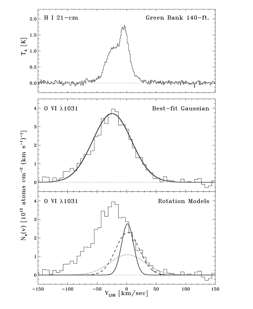
Figure 4: The Green Bank 140-ft H I profile (top) and the O VI apparent column density profile (bottom two panels) observed toward vZ 1128. The O VI $N_{a}(v)$ profiles are shown with the best-fit Gaussian overlaid (middle) and three models of the $N_{a}(v)$ distribution assuming the O VI participates in Galactic rotation (bottom). The best-fit Gaussian has a dispersion $\sigma=31.8\pm 1.1$ (after removal of instrumental effects). The rotation models all assume the O VI is distributed with a scale height of 2.3 kpc. The three models differ in their assumed cloud velocity dispersion (using $\sigma=10$, 20, and 30 km s^-1) and have been scaled to best match the red wing of the O VI profile.

Figure 4 shows the $N_{a}(v)$ distribution of O VI toward vZ 1128 and the NRAO H I 21-cm spectrum. The middle panel shows the O VI $N_{a}(v)$ profile with the best-fit Gaussian distribution overlayed. The properties of this Gaussian are summarized in Table 6, along with the properties of Gaussians fit to the $N_{a}(v)$ profiles of several lower-ionization species. The best-fit Gaussian dispersion, $\sigma\,(\equiv b/\sqrt{2})$, after removal of the instrumental breadth, is $31.8\pm 1.1$ km s^-1 (equivalent to a Doppler parameter $b=45.0$ km s^-1). This limits the temperature of the O VI along the sight line to $T\lesssim 2\times 10^{6}$ K. This is significantly larger than the temperature at which the abundance of O VI peaks in collisional ionization equilibrium, $T\sim 3\times 10^{5}$ K, and the large breadth indicates significant non-thermal broadening of the profile.

The kinematic properties of the O VI profile toward vZ 1128 are significantly different than expected for a highly-ionized thick disk corotating with the underlying thin disk. Because of the high latitude of this star, Galactic rotation is expected to have very little impact on the velocity profiles of any interstellar species. The bottom panel of Figure 4 shows the O VI $N_{a}(v)$ profile with three models of simple rotation of a thick O VI-bearing disk with scale height of $\sim 2.3$ kpc (see Savage et al. 2003). The three models differ in the assumed dispersion of the O VI-bearing gas (with models shown for Gaussian dispersion of $\sigma=10$, 20, and 30 km s^-1). The midplane density in each model is scaled to match the red wing of the O VI profile.

The observed velocity distribution of O VI is clearly inconsistent with these simple models of Galactic rotation. The observed profile shows much more material at negative velocities than is expected for a corotating thick disk of O VI-bearing material. Indeed, the velocity centroid of O VI suggests the bulk of the highly-ionized material along this sight line is falling onto the Galactic disk from the halo. The central velocity of the O VI profile, $\langle v_{\rm LSR}\rangle\approx-26$ km s^-1, is consistent with the center of the broad negative velocity absorption seen in the NRAO H I profile (at $v_{\rm LSR}\sim-25$ km s^-1). It is also interesting to note the relatively good agreement between the central velocities of WNM/WIM tracers and O VI (see Table 6). Thus, it would seem that the infalling gas along this sight line contains a range of ionization states. We discuss the kinematic relationship between the WNM/WIM tracers in §6.4.

The kinematics of O VI along the vZ 1128 sight line are perhaps best discussed in the context of similar high-latitude observations. Wakker et al. (2003) and Savage et al. (2003) present Galactic O VI absorption lines toward $\sim 100$ extragalactic objects. They find that while there is a large spread in the observed central velocities of the O VI observed along high-latitude sight lines, the average of the distribution is $v_{\rm LSR}=0\pm 21$ km s^-1 (standard deviation). Thus, while we observe the O VI to be infalling toward vZ 1128, this should be viewed in the context of the broad distribution of outflowing and infalling O VI gas across the entire high-latitude sky. The central velocity of the vZ 1128 O VI distribution cannot be used, for example, to claim that the entire highly-ionized Galactic thick disk is collapsing onto the plane.

The observed Gaussian dispersion can also be discussed in the broader context of the Wakker et al. and Savage et al. measurements. These authors use a slightly different approach to determining the velocity breadths of the O VI absorption profiles, defining a quantity we refer to as $b^{\prime}$:

$$b^{\prime}\equiv\left[2\,\frac{\int(v-\bar{v})^{2}N_{a}(v)dv}{\int N_{a}(v)dv}\right]^{1/2}$$

These authors find $\langle b^{\prime}\rangle=60\pm 15$ km s^-1 for their sample of extragalactic sight lines (with no correction for instrumental effects). Our measured dispersion corresponds to $b\approx 46.5\pm 1.6$ km s^-1 (before correcting for the instrumental spread function). If derived in the manner used by these authors, we find $b^{\prime}$ for the O VI toward vZ 1128 is $57\pm 3$ km s^-1. Thus, the breadth of the O VI profile toward vZ 1128 is well within one standard deviation of the high-latitude mean derived by Wakker et al. and Savage et al.

6 Warm Ionized and Neutral Gas Toward von Zeipel 1128

One of the goals of this program is to understand the relationship between the observational tracers of warm neutral and ionized gas in the Galactic thick disk. This section discusses the relative elemental abundances in the WNM and WIM as well as the kinematics of the tracers of these phases toward vZ 1128.

The WNM and WIM in the Galactic thick disk are probed by low and intermediate ions, respectively. Low-ionization species include those thought to be the dominant ionization state of each element in the WNM; low ions observed toward vZ 1128 include C II, N I, O I, Si II, P II, Ar I, and Fe II. We describe the next-higher ionization stages as intermediate ions, including the species C III, N II, S III, and Fe III observed toward vZ 1128. These ions are likely to arise in the WIM (and perhaps to some degree in the hot ISM; see Howk & Savage 1999b) along with some of the low ions.

The low ions may arise in both the WNM and WIM (Haffner, Reynolds, & Tufte 1999; Sembach et al. 2000), which is a source of some concern, since these are the ions used to determine gas-phase abundances in the WNM (see discussion in Sembach et al. 2000). The degree of uncertainty associated with this “contamination” (or confusion) of WNM species by gas associated with the WIM varies from element to element. We discuss such contamination for the specific case of iron below.

6.1 Gas-phase Abundances in the Warm Neutral Material

The gas-phase abundance of an element $X$ relative to an element $Y$ is calculated as

$$[X/Y]\equiv\log\,[N(X^{i})/N(Y^{j})]-\log\,(X/Y)_{\odot}-\log\,[x(X^{i})/x(Y^{j})].$$ (4)

In this expression $N(X^{i})$ and $N(Y^{j})$ are the column densities of the ions $X^{i}$ and $Y^{j}$. These column densities are normalized to the relative solar system abundances of the two elements, $(X/Y)_{\odot}$ (Grevesse & Sauval 1998; see Table 7). The quantities $x(X^{i})$ and $x(Y^{j})$ are the ionization fractions of each ion in the gas being studied. The last term is the ionization correction. Typically the dominant WNM ionization state of the two elements is used, and the ionization correction is assumed to be insignificant. Exceptions to this general rule include studies of Ar I, which is easily photoionized in WNM conditions (Sofia & Jenkins 1998).

Table 7 and Figure 5 summarize the gas-phase abundances in the WNM derived in the usual way. That is, we have compared the column densities of low-ionization species with that of H I in this direction. Studies of the WNM typically use H I or a non-depleted metal ion as a reference for studying interstellar grain composition. The relative deficit of metals in the ISM compared with the solar system is assumed to be caused by the incorporation of these metals into dust grains (the solid phase). Applying the standard technique yields only an approximate determination of $[X/{\rm H}]$ for the WNM in this direction because of the assumption that $\log\,[x(X^{i})/x(\mbox{H$\;${\small\rm I}})]=0$ in Eqn. (4).

Figure 5 shows the WNM gas-phase abundances for the vZ 1128 sight line along with the range of values seen along other thick disk (or “halo”) sight lines. The gas-phase abundances toward vZ 1128 are not out of the ordinary for high-latitude sight lines. We point out that these measurements represent averages over the entire sight line. There is evidence that many of the metals are distributed differently in velocity space than the H I, especially the species heavily incorporated into dust grains (see below).

6.2 Ionization Effects

The measurements given in Table 7 provide a baseline for determining the extent to which ionization effects influence such abundance determinations and for comparing the properties of the WNM and WIM along the vZ 1128 sight line. We first discuss the average ionization state of the gas along this sight line because it bears on the gas-phase abundances derived above.

Using the Eqn. (3), it is possible to estimate the column density of protons associated with the intermediate ions toward vZ 1128. Such an estimate, combined with measures of $N(\mbox{H$\;${\small\rm I}})$, provides a rough measure of the total hydrogen column density along the sight line. For determining the proton column density of the WIM, we make use of the S III column density reported in Table 5.

The most basic assumption, i.e., that all of the WIM sulfur is in the form of S III [$x(\mbox{S$\;${\small\rm III}})=1$] and sulfur is undepleted (Howk, Savage, & Fabian 1999), results in a lower limit to the proton column associated with the WIM: $\log N(\mbox{H$\;${\small\rm II}})>19.1$. Sembach et al. (2000) have presented models of the ionization of the WIM assuming ionization by early-type stars. If we adopt the sulfur ionization fractions from their composite standard model [$x(\mbox{S$\;${\small\rm III}})\sim 0.18$] for our calculation, we find $\log N(\mbox{H$\;${\small\rm II}})=19.9$. For comparison, similar calculations performed using the lower and upper limits provided by N II and P III yield $18.6<\log N(\mbox{H$\;${\small\rm II}})\lesssim 20.8$, consistent with the valued derived using S III.

The proton columns estimated using S III above imply a total hydrogen column density of $\log N(\mbox{H$\;${\small\rm I}+H$\;${\small\rm II}})=20.0$ to 20.2 and $\langle x(\mbox{H$\;${\small\rm II}})\rangle\equiv N(\mbox{H$\;${\small\rm II}})/N(\mbox{H$\;${\small\rm I}+H$\;${\small\rm II}})\gtrsim 0.12$ to $\sim 0.46$, with the latter being the preferred estimate. These values are roughly consistent with the estimates of $x(\mbox{H$\;${\small\rm II}})$ derived from the H$\alpha$ intensity in this general direction (§2).

With this estimate of the total hydrogen column density of the WNM and WIM (since the hot ISM likely contributes little, as discussed in §5), we can further estimate the total gas-phase iron abundance. The total iron column density along this sight line is $\log N({\rm Fe})_{total}\approx\log N(\mbox{Fe$\;${\small\rm II}+Fe$\;${\small\rm III}})=14.95\pm 0.04$, assuming higher ionization states represent a small fraction of the total. Thus, the gas-phase abundance of iron along the sight line to vZ 1128 (averaged over all phases and regions) is

$$-0.76\lesssim{\rm[Fe/H]}_{total}<-0.56.$$

This can be compared to the value $[{\rm Fe/H}]_{WNM}=-0.64\pm 0.06$ derived using Fe II and H I with no ionization correction. The ionization corrections for the derived WNM gas-phase abundance appear to be $\lesssim\pm 0.1$ dex (averaged over the entire sight line).

6.3 Gas-phase Abundances in the Warm Ionized Material

It is also possible to estimate the gas-phase abundances of refractory elements in the WIM by comparing the columns of intermediate-ionization stages of depleted and non-depleted species and applying an ionization correction. Howk & Savage (1999b) have presented determinations of [Al/S] in the WIM using this approach, arguing on the basis of the derived values that dust is present in the ionized medium of the Galaxy. This conclusion has been confirmed by the detection of far-infrared emission from dust associated with the WIM (Lagache et al. 2000).

Our observations of Fe III and S III provide a similar opportunity to determine the relative gas-phase abundances of iron and sulfur in the WIM. We determine [Fe/S]_WIM in the manner outlined in Eqn. (4):

$${\rm[Fe/S]}_{WIM}\equiv\log\,[N(\mbox{Fe$\;${\small\rm III}})/N(\mbox{S$\;${\small\rm III}})]-\log\,({\rm Fe/S})_{\odot}-\log\,[x(\mbox{Fe$\;${\small\rm III}})/x(\mbox{S$\;${\small\rm III}})].$$ (5)

In this case the ionization correction term, $\log[x(\mbox{Fe$\;${\small\rm III}})/x(\mbox{S$\;${\small\rm III}})]$, is significant.

The composite standard WIM model (Sembach et al. 2000) has $\log[x(\mbox{Fe$\;${\small\rm III}})/x(\mbox{S$\;${\small\rm III}})]=+0.45$, which yields

$${\rm[Fe/S]}_{WIM}\sim-0.74\pm 0.3$$

for the sight line to vZ 1128. The error bar is an estimate of the uncertainties in the ionization corrections due to the sensitivity of $x(\mbox{Fe$\;${\small\rm III}})/x(\mbox{S$\;${\small\rm III}})$ to the adopted effective temperature of the ionizing source following Howk & Savage (1999b). This determination is in excellent agreement with the WNM determination and the values of ${\rm[Fe/H]}_{total}$ and ${\rm[Fe/H]}_{WNM}$ derived above. The implications of this similarity are discussed more thoroughly in §8.

6.4 Kinematics of the Warm Ionized and Warm Neutral Gas

We now turn our attention to the kinematic relationship between the low- and intermediate-ions toward vZ 1128. Figure 6 shows the apparent column density profiles of a range of ions observed toward vZ 1128, including species tracing the WNM and the WIM. Also shown is the O VI profile, which traces the warm-hot ISM. Measurements of the velocity centroids and breadths of the $N_{a}(v)$ profiles of several species are given in Table 6. The peak apparent optical depths of each transition are also given as a guide for judging the relative importance of saturation effects on the derived kinematic properties.

It is clear that the resolution of FUSE is insufficient to clearly resolve the detailed component structure of this sight line. Examining the $N_{a}(v)$ profile of the strong Si II 1020 Å line (which is susceptible to unresolved saturation at the highest optical depths), there is clear evidence for velocity substructure that cannot be clearly separated at FUSE resolution. For this reason, we concentrate our discussion of the kinematics of the WNM/WIM gas on the central velocity and breadth of the absorption. The majority of the species presented in Figure 6 and Table 6 have similar central velocities ranging from $v_{\rm LSR}\approx-31$ to $-21$ km s^-1, including O VI. The one exception to this agreement in the velocities of the observed species is Ar I, which is centered near $v_{\rm LSR}\approx-10$ km s^-1. Because of its large ionization cross section (Sofia & Jenkins 1998), Ar I is relatively easy to ionize in diffuse interstellar gas, even though its ionization potential is larger than that of H I. This is the most likely cause for the apparent deficit of Ar I seen in Figure 5, particularly since argon is unlikely to bind to grains effectively (Sofia & Jenkins 1998). All of the species displayed in Figure 6 show absorption at the velocities at which Ar I has a maximum optical depth.

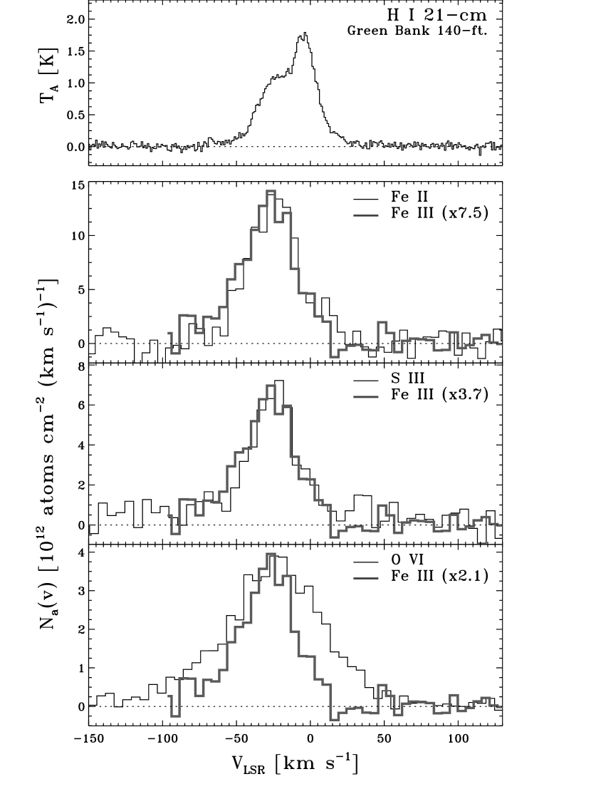
Figure 7: Apparent column density profiles of Fe III compared with Fe II, S III, and O VI. In each case the Fe III profile has been scaled to match the other species. The WNM and WIM species trace each other quite well (within the limitations of the FUSE resolution), though there may be a slight excess of Fe III near $v_{\rm LSR}\approx-50$ km s^-1 compared with the others. The Fe III and O VI have nearly the same central velocity, though the latter, which traces hotter gas, is much broader.

To the extent that the FUSE resolution allows us to study such coincidences, the breadths of the profiles of species tracing the WNM and WIM are quite similar. Figure 7 compares the apparent column density profiles for Fe II, Fe III, and S III. With the exception of a possible weak excess in Fe III at $v_{\rm LSR}\sim-50$ km s^-1, the profiles of these species track one another remarkably well. The similarity of the observed profiles suggests the WNM and WIM share a similar component structure. Large component-to-component variations in the ratio of the WNM and WIM tracers can be ruled out for the dominant component groups along this sight line (strong variations in the ratio among low column density components cannot be ruled out).

An interpretation of the kinematics of the WNM/WIM tracers discussed in this section is that the species centered near $v_{\rm LSR}\sim-26$ km s^-1 principally trace gas in the Galactic thick disk and are associated with the broad H I seen at similar velocities. The material closer to the LSR zero point, including the narrower peak of the H I distribution and the majority of the Ar I, is likely tracing gas associated with lower-ionization, higher-depletion material in the Galactic disk in this direction. The principal WNM tracers accessible by FUSE probe elements that are readily incorporated into dust grains. These ions are therefore biased toward gas in the Galactic thick disk, which is more likely to be ionized than the thin disk and to have higher gas-phase abundances due to the processing of dust grains (e.g., Sembach & Savage 1996).

It is significant that there seems to be little evidence for gas that can be associated with only the neutral or ionized gas of the Galactic thick disk.

7 The Lack of High-Velocity Gas

7.1 High Velocity Clouds

There is no evidence for discrete high-velocity cloud material along the vZ 1128 sight line in O VI or lower-ionization species. Sembach et al. (2003) have discussed the presence of high-velocity O VI toward extragalactic objects. They find high-velocity O VI toward $\sim 60\%$ of the sight lines studied (although some were initially chosen to probe the known H I high-velocity clouds). In a few cases, the lack of high-velocity material toward vZ 1128 is confused by the presence of high negative-velocity stellar photospheric absorption features (see, e.g., the C II 1036.337 Å transition in Figure 3).

For O VI, our $3\sigma$ upper limit on the column density of high-velocity ($|v_{\rm LSR}|\gtrsim 125$ km s^-1) material is $\log N(\mbox{O$\;${\small\rm VI}})\lesssim 13.3$, assuming $\sigma\sim 32$ km s^-1 ($b\sim 45$ km s^-1). We note that $\sim 20\%$ of the sight lines studied by Sembach et al. (2003) show the presence of very broad, high-positive-velocity wings in O VI extending from $|v_{\rm LSR}|\sim 100$ to $\sim 250$ km s^-1. Most of these wings are found in the northern Galactic sky. We see no evidence for low optical depth, high-velocity wings such as these toward vZ 1128.

There are no H I high-velocity cloud complexes toward vZ 1128 identified through 21-cm H I emission line observations. Thus, even though a large fraction of the extragalactic targets show high-velocity O VI, it is unclear if we expect to see such material toward vZ 1128. To demonstrate the lack of high-velocity material toward vZ 1128, we show normalized spectra of two higher-order Lyman series H I lines toward vZ 1128, together with the profiles of C II $\lambda 1036.337$, C III $\lambda 977.020$, and O VI $\lambda 1031.926$ in Figure 8. The H I profiles have been normalized by the same model stellar atmosphere used for the N II profile (see §4). Even though this model is a reasonable descriptor of the broad stellar H I absorption seen in the FUSE data, we caution that the application of an incorrect model profile could leave unrealistic broad absorption in the spectrum, particularly at negative velocities where the absorption from the star is strongest. The vertical lines in Figure 8 denote the approximate range of C II absorption at its half intensity points.

There is little visible H I beyond the extent of the C II profile. The H I profiles seem to be confined to $-125\lesssim v_{\rm LSR}\lesssim+65$ km s^-1 (with the caveat that the negative velocity extent is dependent upon the adopted stellar profile). Outside of this velocity range, we find an upper limit to the H I column density of any high-velocity material of $\log N(\mbox{H$\;${\small\rm I}})\lesssim 14.7$ ($3\sigma$). Neither do we see evidence for high-velocity absorption in low-ionization metal species. Assuming such absorption would have breadths similar to the values listed in Table 6, we derive limits of $\log N(\mbox{Fe$\;${\small\rm II}})\lesssim 13.4$, $\log N(\mbox{Fe$\;${\small\rm III}})\lesssim 13.5$, and $\log N(\mbox{{N~{}II}})\lesssim 13.4$ ($3\sigma$ limits) for material with $|v_{\rm LSR}|\gtrsim 125$ km s^-1. The Fe III limits only apply to high positive velocities since the profile is blended with interstellar Fe II and stellar Fe III at negative velocities.

The intermediate-velocity cloud complex K (Wakker 2002) is found at lower Galactic latitudes in H I maps at $v_{\rm LSR}\approx-70$ km s^-1. The map of this complex in Wakker (2002) shows the nearest contour enclosing $N(\mbox{H$\;${\small\rm I}})>5\times 10^{18}$ is $\sim 10^{\circ}$ from vZ 1128. It is difficult to say if complex K is detected toward vZ 1128. The very strongly-saturated C II 1036.337 Å transition shows some evidence for weak absorption at velocities consistent with an origin in complex K. Small wings at the appropriate velocity may also be seen in the stronger O I and Si II transitions (see Figure 3). However, the absorption at these velocities is not sufficiently well delineated to allow us to study it in detail.

7.2 Globular Cluster Gas

We note that no absorption associated with the circumstellar environment of vZ 1128 or with the globular cluster M 3 is seen in our data, assuming any gas in the vicinity of M 3 would be found near its systemic velocity ($v_{\rm LSR}=-137.0\pm 0.3$; Soderberg et al. 1999). For O VI, our $3\sigma$ upper limit on the column density of material associated with the globular cluster is $\log N(\mbox{O$\;${\small\rm VI}})\lesssim 13.3$, assuming $\sigma\sim 32$ km s^-1 ($b\sim 45$ km s^-1). Neither do we see evidence for absorption in lower-ionization species. Assuming such absorption would have breadths similar to the values listed in Table 6, we derive limits of $\log N(\mbox{Fe$\;${\small\rm II}})\lesssim 13.4$ and $\log N(\mbox{{N~{}II}})\lesssim 13.4$ ($3\sigma$). The Lyman series of hydrogen cannot be used to search for globular cluster or circumstellar material because of the strong stellar H I absorption.

These determinations can be used to estimate upper limits on the mass of interstellar material in the globular cluster. The calculation follows that for determining the hydrogen column density associated with O VI in the hot ISM (see §5) with the additional step of multiplying that column by a projected area for the cluster. We assume a metallicity $[{\rm M/H}]\approx-1.57$ (Harris 1996) and that the upper limits of the above ions are applicable to the whole cluster. The distance of vZ 1128 from the cluster core ($\sim 3\farcm 9$ or $\sim 11$ pc) and the limits on O VI imply an intracluster gas mass ($M_{ICM}$) of $M_{ICM}\lesssim 4.4\,x(\mbox{O$\;${\small\rm VI}})^{-1}$ M_⊙. If we limit this calculation to temperatures $5.3\lesssim\log T\lesssim 5.6$ [the range over which $x(\mbox{O$\;${\small\rm VI}})\gtrsim 0.05$ for both the equilibrium calculations of Sutherland & Dopita (1993) and the non-equilibrium calculations of Shapiro & Moore (1976)], we have $M_{ICM}\lesssim 90$ M_⊙. Similarly we can use the limits on N II assuming the gas is fully ionized (i.e., hydrogen is fully ionized and the ionization of nitrogen is tied to that of hydrogen via its charge exchange reaction) to limit the mass of the intracluster medium to be $M_{ICM}\lesssim 35$ M_⊙.

Our calculations assume that the limits to the gas column density toward vZ 1128 are applicable to the entire projected area within the 11 pc distance to the cluster core. If the column of gas is higher toward the center of the cluster or if vZ 1128 lies on the front side of the cluster, then our limits are not appropriate. Our limits on the mass of ICM material in M 3 are similar to other recent limits on the amount of ionized gas in globular clusters (e.g., Knapp et al. 1996) and the one detection (Freire et al. 2001). The density of ionized gas detected in 47 Tuc by Freire et al. (2002) implies a mass of $\sim 10$ M_⊙ if the gas extends as far as 11 pc from the cluster center, the projected distance of vZ 1128 from the center of M 3.

7.3 High-Velocity Dispersion Gas

Kalberla et al. (1998) have used the LDS H I observations to argue for the presence of a high velocity-dispersion component of the Galactic ISM. They find evidence for diffuse H I with $\sigma\approx 60$ km s^-1 and $\log N(\mbox{H$\;${\small\rm I}})\approx 19.15$. If exponentially distributed, Kalberla et al. argue such a distribution would have a midplane density of $\sim 1.2\times 10^{-3}$ cm^-3 and a scale height of $\sim 4.4$ kpc.

Such a component of the ISM should be readily visible as strongly-saturated Lyman-series absorption toward distant stars and AGN. Savage et al. (2000) have argued on the basis of the measured equivalent widths of the strong Mg II doublet near 2800 Å that such a phase of the ISM cannot exist unless the abundance of Mg in this material is far below solar ($\sim 0.05$ solar).

Using the Lyman series of H I as a probe of this gas alleviates the issue of abundances. If such material were present toward vZ 1128, the H I 930.748 Å line seen in Figure 8 would have $\lesssim 1\%$ residual intensity over the range $-200\lesssim v_{\rm LSR}\lesssim+200$ km s^-1. The H I Lyman series towards vZ 1128 (conservatively) limits the column density of such material in this direction to be $\log N(\mbox{H$\;${\small\rm I}})\lesssim 16.7$ cm^-2.

While we can say with some confidence that a phase of the ISM which is smoothly distributed and has a dispersion and column density like those discussed in Kalberla et al. (1998) does not exist toward vZ 1128, their detection as a whole cannot be ruled out by the present data alone. To identify this phase of the ISM, Kalberla et al. averaged over $\sim 10^{\circ}\times 10^{\circ}$ sections of the sky to identify this gas. If this high velocity-disperion H I distribution is contained in clouds which cover a relatively small fraction of the sky and as an ensemble have a cloud-to-cloud dispersion of order 60 km s^-1, we would not necessarily expect to find material associated with this distribution along a single sight line. Lockman (2002) has recently idenfitied a population of discrete thick disk clouds in the inner Galaxy. Whether the ensemble of such clouds at the solar circle (if such a population exists) can match the distribution inferred by Kalberla et al. (1998) is not known.

An investigation of the validity of the Kalberla et al. (1998) result is best pursued using a large database of FUSE observations of extragalactic sources (where there is no broad Lyman-series absorption in the background source itself). Should no such sight lines through the entire Galactic halo show evidence for such gas, the reality of such an H I layer will need to be reevaluated.

8 Discussion

8.1 The Phases of the Galactic Thick Disk

Because we are able to measure the column densities of species associated with all phases of the ISM toward vZ 1128, we can estimate the contribution each phase makes to the total hydrogen (neutral plus ionized) along this sight line. In this way we can construct a census of the phases in this direction. Table 8 gives such a summary of the phases toward vZ 1128, which contains the hydrogen column for each phase (as estimated above) and the fraction of the total each represents along this sight line. We also summarize the best estimates of the scale heights of each phase from the literature.

The fraction of the total hydrogen along the vZ 1128 sight line estimated to be associated with warm ionized gas is $\sim 10\%-45\%$. In this case, the higher end of this range is more robust since it is based upon a model of the ionization fraction of sulfur in the WIM. The lower value assumes that all of the sulfur is in S III, which yields a firm lower limit to the ionized hydrogen column density associated with the WIM. This range of fractional hydrogen column density is similar to the observed values derived by comparing the electron column densities (derived from pulsar dispersion measures) with H I column densities toward distant globular clusters. Reynolds (1991b) summarizes five such measurements which give fractions of ionized hydrogen in the range $19\%-40\%$.

The highly-ionized, transition-temperature gas traced by O VI represents a relatively small fraction of the total hydrogen column density along this path through the Galactic thick disk and corona. It should be noted that the O VI absorption is likely not tracing material at X-ray emitting temperatures ($\gtrsim 10^{6}$ K); therefore, the total amount of hot gas could be higher. Furthermore, because we have adopted the highest ionization fraction for estimating the hydrogen column from O VI, the stated values should be treated as (uncertain) lower limits.

8.2 The Relationship Between Neutral and Ionized Gas in the Galactic Thick Disk

Our determinations of the depleted gas-phase abundances of iron in the WNM and WIM are very similar, suggesting the content of iron-bearing dust is similar in these two phases. This tends to support the notion that the gas and dust that make up the WNM and WIM of the Galactic thick disk have experienced similar dust destruction and formation histories. If the processes that feed WNM and WIM material into the thick disk were significantly different (i.e., if one were more violent than the other), the dust content, and hence the gas-phase abundances, of these phases might be significantly different.

We point out, however, that our determination of ${\rm[Fe/S]}_{WIM}$ has a relatively large uncertainty due to the photoionization modeling. Using refined models and species that are less susceptible to changes in the ionizing spectrum (e.g., Al III; see Howk & Savage 1999b) for determining the WIM abundances will provide more precise results. It is also worth pointing out that the WNM abundance determinations may be affected at the $\sim 0.1$ dex level by our neglect of the ionization correction term in Eqn. (4).

The kinematic similarities between the tracers of the WNM (e.g., Fe II) and the WIM (e.g., Fe III, S III) along this sight line also suggest a relatively close relationship between these phases of the Galactic thick disk. The distribution of clouds in velocity space is likely very similar between the two phases. We see no significant difference in the large-scale velocity dispersion of the warm ionized gas and warm neutral gas toward vZ 1128. This indicates that these two phases have similar vertical extents along this high-latitude sight line, unless processes are at work that affect the vertical distribution of two phases differently while suppressing large-scale velocity profile differences.

The kinematic similarities suggest a relationship between these phases toward vZ 1128 that is similar to that seen toward HD 93521 (Spitzer & Fitzpatrick 1993) and $\rho$ Leo (Howk & Savage 1999b). Along these sight lines, tracers of electron-rich gas (e.g., C II^∗, Al III, S III) show a velocity component structure that is virtually indistinguishable from tracers of the WNM (e.g., Zn II, Si II, Fe II). The apparent similarity of the Fe II and Fe III profiles as observed by FUSE does not rule out moderate, unresolved component-to-component variations in the ratio of these species.

The apparent constancy of the Fe III to Fe II ratio with velocity also implies that there are no strong intermediate- or high-velocity features with unusual Fe III content (i.e., none that are significantly more highly-ionized than the bulk of the thick disk material along this sight line). The resolution of FUSE does not allow us to place strong limits on such components at low velocities, and the overlap of the strong Fe II 1121.975 Å transition at negative velocities relative to Fe III also makes the limits more significant at positive velocities.

There is one caveat to these kinematic comparisons of the WNM and WIM tracers. If the WIM does indeed represent as much as $\sim 45\%$ of the total hydrogen in this direction, much of the column density of singly-ionized species we have associated with the WNM may arise in the WIM. For example, the standard composite WIM model of Sembach et al. (2000) predicts $x(\mbox{{Fe~{}II}})\approx 0.5$. If the fraction of hydrogen toward vZ 1128 is $\sim 50\%$, then $\sim 25\%$ of the Fe II is expected to arise in the WIM. In the case of Si II, $x(\mbox{{Si~{}II}})\sim 0.9$, implying that $40\%$ of the column density of this ion could arise in the WIM. It is not difficult to understand why the tracers we have naively associated with the WNM might have very similar kinematics to the intermediate ions if they are indeed contaminated by this amount of WIM gas.

The observed O VI profile, which traces transition-temperature gas in the warm-hot ISM, is centered at velocities consistent with the centroids of the WNM/WIM tracers, but has a much larger velocity dispersion compared with the tracers of the low and intermediate ions. The large breadth of the O VI profile may be the result of large turbulent (or other non-thermal microphysical) motions or large-scale cloud-to-cloud motions. The breadth of the O VI profile toward vZ 1128 is consistent with the $N(\mbox{O$\;${\small\rm VI}})$-line width relation identified by Heckman et al. (2002).

The agreement between the central velocities of O VI and the lower ionization species is intriguing, though perhaps coincidental. The correspondence of central velocities of all of the tracers of the thick disk ISM in this direction is naturally explained if the O VI arises in interfaces between the warm gas (neutral and ionized) and a much hotter medium (X-ray emitting material at $T\gtrsim 10^{6}$ K). Because of the short cooling time of gas in the range of temperatures at which O VI is abundant, many classes of theoretical models invoke such an arrangement (see summary in Spitzer 1996). [Indeed, such an arrangement calls to mind the clouds envisioned by McKee & Ostriker (1977).]

Examining Figure 8 one finds that the total velocity extent of the strong C II 1036.337 Å and O VI 1031.926 Å profiles is similar. That is, most of the absorption seen in O VI is seen at velocities where there is also some lower-ionization material (as traced by C II). The much larger apparent dispersion of the O VI profile compared with lower-ionization lines of similar peak optical depths is likely due to components further from the velocity centroid which exhibit higher O VI to low ion column density ratios. If one assumes a relatively constant quantity of O VI per interface (e.g., Shelton & Cox 1994), then the observed O VI profile traces the distribution of interfaces as a function of velocity. The individual interfaces much overlap in velocity so that they are not visible as individual components (perhaps being within $\Delta v\sim 2\sigma$ of one another, or $\sim 25$ km s^-1 for $T\sim 3\times 10^{5}$).

Howk et al. (2002b; see also Howk et al. 2002a) have noted that the distribution of O VI and Fe II absorption toward stars in the Large Magellanic Cloud [$(l,b)\approx(280^{\circ},-33^{\circ})$] also requires that the O VI be closely associated with low-ionization material. In these directions, the centroids of the Milky Way O VI profiles are shifted relative to the Fe II profiles, although the total extent of the O VI and Fe II absorption seem to be well correlated. That is, the O VI and Fe II absorption seemed to trace many of the same structures, though the changing O VI/Fe II ratio causes the velocity centroids to be different.

If the O VI and low-ionization species trace different portions of the same structures, the larger dispersion of O VI cannot be simply explained by a larger temperature in the O VI-bearing region. Significant variations must exist in the low-ion to O VI column density ratio, with the outlying O VI components tracing higher-ionization gas (i.e., material with a higher O VI to low ion ratio). This is required not only so that the velocity dispersion be lower in the WNM/WIM tracers, but also to be consistent with the larger O VI scale height compared with the WNM or WIM. Given the much larger scale height of the O VI-bearing gas compared with the WIM [$h_{z}(\mbox{O$\;${\small\rm VI}})\approx 2.3h_{z}({\rm WIM})$; see Table 8], the ratio of O VI to WNM/WIM tracers cannot be constant with height; a larger ratio is required for material further from the plane.

Furthermore, if one solely invokes differences in the temperature of the O VI-bearing gas, the required temperatures are too high to maintain large amounts of O VI. The largest instrumentally-corrected dispersion in the profiles of lower-ionization species with peak optical depths similar to that of O VI (in order to avoid complications from strong saturation) is that of S III: $\sigma_{o}=14.7\pm 1.7$. If the observed O VI is associated with the same components making up the S III profile, an additional broadening of $\sigma\sim 28$ km s^-1 is required to explain the breadth of the O VI profile. This would require $T\sim 1.5\times 10^{6}$ K in each component. At such high temperatures O VI is not expected to be abundant (Sutherland & Dopita 1993; Shapiro & Moore 1976).

The observed arrangement of interstellar absorption toward vZ 1128 can perhaps be best explained by a scenario in which O VI and the lower-ionization species arise in the same structures, with the O VI arising in an interface between the warm and hot phases of the ISM. The material further from the line centroid is found further from the plane of the Galaxy and is characterized by a higher ionization state (as one would expect for lower warm material per constant-column O VI interface). In this scenario, the coincidence of the velocity centroids of O VI and lower-ions requires that most WNM/WIM clouds of the Galactic thick disk have a corresponding O VI-bearing interace, implying that each cloud is embedded within a hot medium. Further analysis of the relationship between O VI and the lower-ionization gas along a larger sample of sight lines is required to determine whether or not this agreement is simply coincidence.

8.3 Ionization Corrections to Gas-Phase Abundance Determinations

As discussed in §6.1, the [Fe/H] abundances derived using the traditional measures (i.e., Fe II/H I) provide a determination that is within $\sim\pm 0.1$ dex of the value derived by accounting for all of the pertinent ionization stages of iron and hydrogen [i.e., (Fe II + Fe III)/(H I + H II)]. This allowable range of ionization corrections for determinations of [Fe/H] is relatively small, implying little ambiguity in studies of gas-phase abundances in varying Galactic environments. For iron, which is very heavily incorporated into dust grains, this ionization correction is indeed small compared with the typical effects of dust. Iron is typically underabundant (depleted) by more than 0.5 dex for WNM material in the Galactic halo and 1.0 dex for WNM material in the Galactic disk (Savage & Sembach 1996). However, it is important to note that the uncertainties due to the neglect of ionization corrections are much larger than typical error bars for such measurements.

The ionization corrections implied here for studying iron in the WNM agrees well with the limits to the ionization corrections derived by Sembach & Savage (1996). We also note reasonable agreement with the ionization corrections estimated for the sight line to HD 93521 by Sembach et al. (2000), depending on the specific model adopted (see their Table 7). However, we caution that the Sembach et al. discussion of the HD 93521 sight line applies to corrections for the ions of sulfur; it is not necessarily the case that ionization corrections derived for iron will apply to the full range of observable singly-ionized species when compared with H I. In particular, the ionization fraction of Fe II in the WIM is expected to be significantly lower than other singly-ionized species such as S II, Si II, and P II (Sembach et al. 2000). Thus, the ionization corrections for these species may be larger than that for iron.

More extensive studies of the ionization corrections along high-latitude sight lines would clearly be useful in determining the applicability of our values to broader studies of the Galactic thick disk.

9 Summary

We have presented Far Ultraviolet Spectroscopic Explorer observations of the distant post-AGB star von Zeipel 1128, which resides in the globular cluster Messier 3. We have derived column densities and kinematic information for the prominent phases of the ISM along this sight line using the absorption lines present in the FUSE data. The major conclusions of this work are as follows.

1. Thick disk material toward vZ 1128 is centered near $v_{\rm LSR}\sim-26$ km s^-1, implying infall of this material onto the Galactic plane in this general direction. Species tracing the prominent warm neutral, warm ionized, and transition temperature ionized phases are seen at very similar velocities along this sight line.

2. As much as $\sim 45\%$ of the hydrogen toward vZ 1128 may be associated with the WIM. The tracers of WNM and WIM gas toward vZ 1128 have very similar kinematic profiles, showing both the same central velocity and very similar breadths.

3. After accounting for all of the ionization stages of iron and hydrogen, we find that the ionization corrections to the standard method of determining the gas-phase abundance of [Fe/H] are likely of order 0.1 dex.

4. The gas-phase abundance of [Fe/S] in the WIM is estimated by comparing the ratio Fe III/S III and applying an ionization correction (using the models of Sembach et al. 2000). The gas-phase abundance of iron in the WIM is indistinguishable from that of the WNM toward vZ 1128. The WIM gas-phase abundance of iron, $[{\rm Fe/S}]_{WIM}\approx-0.74\pm 0.3$, suggests significant incorporation of iron into dust in this phase of the Galactic thick disk.

5. The similarities of the kinematics and gas-phase abundances of the WNM and the WIM suggest the two phases of the Galactic thick disk are closely related along this sight line. The WNM and WIM in this direction likely have similar vertical extents and similar Fe-bearing dust content.

6. The broad ($\sigma=32$ km s^-1) O VI absorption toward vZ 1128 is centered at the same velocities as the WNM and WIM tracers along this sight line. The low- and high-ionization gas along this sight line seem to be closely related given the similarity in their central velocities and total velocity extent. It seems likely that the O VI arises in interfaces between hot and warm gas, with the shape of the O VI profile tracing the distribution of interfaces in velocity.

7. We see no high-velocity material that could be associated with the circumstellar environment of vZ 1128 or with the globular cluster Messier 3 in which vZ 1128 resides. No high-velocity clouds are seen along this sight line in the low- or high-ionization states observed by FUSE. No high-velocity dispersion gas is seen in the H I Lyman-series absorption.

Table 1: Properties of von Zeipel 1128

Property	Value	Reference
Cluster	M 3 (NGC 5272)	$\cdots$
RA (J2000)	13 42 16.84	$\cdots$
Dec. (J2000)	$+28$ 26 00.8	$\cdots$
$(l,b)$	$(42\fdg 5,\ +78\fdg 7)$	$\cdots$
Distance [kpc]	10.2	1
$z$ [kpc]	10.0	1
Sp. Type	O8p	2
V [mag.]	14.93	3
B-V [mag.]	$-0.27$	3
$T_{eff}$ [K]	$35,000\pm 1,000$	4
$\log g$	$4.0\pm 0.25$	4
$\log L/L_{\odot}$	$3.21\pm 0.12$	4
$v_{\rm LSR,cluster}$ [km s-1]	$-137.0\pm 0.3$	5
$v_{\rm LSR,vZ1128}$ [km s-1]	$-140\pm 8$	6

Table 2: Log of FUSE Observations

Visit	Date	No. of	Exp. Time
ID		Exp.	[sec]
P1014101	6/18/2000	7	9119
P1014102	6/19/2000	9	7684
P1014103	6/22/2000	9	14723
Total:		25	31526

Table 3: Stellar Radial Velocity Measurements

Species	$\lambda$	Ref.	$v_{\rm LSR}$ [km s-1]
P IV	1030.515	1	$-140.7\pm 2.3$
P IV	1033.112	1	$-135\pm 7$
P IV	1035.516	1	$-136\pm 3$
S IV	1062.678	2	$-142.1\pm 1.1$
S IV	1072.996	2	$-138.3\pm 1.1$
S IV	1073.528	2	$-139.1\pm 1.0$
P V	1117.977	3	$-141.6\pm 1.5$
P V	1128.008	3	$-141.6\pm 1.3$
C III	1174.933	4	$-139.2\pm 1.4$
C III	1176.370	4	$-141.1\pm 1.3$

Table 4: Selected Interstellar Absorption Lines Towards vZ 1128

Species	$\lambda$	$\log\lambda f$	$W_{\lambda}$ [mÅ]			$\log N_{a}(v)$		$v_{-},v_{+}$
	[Å]		[Det 1]	[Det 2]		[Det 1]	[Det 2]	[km s-1]
C II	1036.337	2.106	$399\pm 5$	$400\pm 7$		$>14.55$	$>14.55$	$-120,+45$
C III	977.020	2.872	$457\pm 9$	$452\pm 7$		$>13.85$	$>13.85$	$-100,+120$
N I	964.626	0.959	$110\pm 6$	$115\pm 5$		$15.28\pm 0.03$	$15.35\pm 0.03$	$-65,+45$
N I	1134.165	1.238	$154\pm 4$	$172\pm 3$		$15.22\pm 0.03$	$15.33\pm 0.03$	$-55,+50$
N I	1134.415	1.528	$207\pm 5$	$204\pm 4$		$15.06\pm 0.03$	$15.15\pm 0.04$	$-50,+50$
N I	1134.980	1.693	$220\pm 6$	$231\pm 4$		$14.94\pm 0.04$	$15.08\pm 0.18$	$-95,+45$
N II	1083.994	2.100	$393\pm 11$	$393\pm 13$		$>14.52$	$>14.52$	$-110,+55$
O I	924.950	0.155	$134\pm 9$	$145\pm 7$		$16.25\pm 0.04$	$16.37\pm 0.03$	$-65,+40$
O I	929.517	0.329	$150\pm 12$	$167\pm 7$		$16.16\pm 0.04$	$16.25\pm 0.03$	$-95,+50$
O I	950.885	0.176	$146\pm 8$	$157\pm 6$		$16.23\pm 0.03$	$16.34\pm 0.02$	$-65,+30$
O I	1039.230	0.980	$249\pm 4$	$245\pm 5$		$>15.89$	$>15.84$	$-85,+40$
O VI	1031.926	2.137	$260\pm 7$	$263\pm 8$		$14.49\pm 0.03$	$14.51\pm 0.03$	$-160,+100$
O VI	1037.617	1.836	$150\pm 6$	$150\pm 7$		$14.48\pm 0.03$	$14.47\pm 0.03$	$-95,+50$
Si II	1020.699	1.460	$153\pm 4$	$158\pm 6$		$15.20\pm 0.02$	$15.22\pm 0.03$	$-80,+30$
P II	1152.818	2.435	$38\pm 6$	$60\pm 4$		$13.20\pm 0.07$	$13.41\pm 0.04$	$-75,+30$
P III	998.000	2.047	$<34$	$<25$		$<13.53$	$<13.41$	$\cdots$
P V	1117.977	2.723	$<25$	$<25$		$<12.68$	$<12.68$	$\cdots$
S III	1012.495	1.556	$92\pm 4$	$91\pm 6$		$14.47\pm 0.02$	$14.47\pm 0.03$	$-90,+20$
S IV	1062.664	1.799	$<28$	$<34$		$<13.67$	$<13.75$	$\cdots$
S VI	944.523	2.311	$<43$	$<45$		$<13.40$	$<13.40$	$\cdots$
Ar I	1048.220	2.408	$90\pm 4$	$97\pm 4$		$13.70\pm 0.03$	$13.71\pm 0.02$	$-70,+25$
Ar I	1066.660	1.851	$51\pm 3$	$44\pm 5$		$13.94\pm 0.04$	$13.88\pm 0.05$	$-55,+40$
Fe II	1055.262	0.898	$54\pm 4$	$49\pm 5$		$14.92\pm 0.03$	$14.88\pm 0.04$	$-90,+15$
Fe II	1063.176	1.765	$165\pm 5$	$160\pm 6$		$14.73\pm 0.03$	$14.68\pm 0.04$	$-90,+35$
Fe II	1096.877	1.545		$132\pm 4$			$14.76\pm 0.02$	$-75,+25$
Fe II	1125.448	1.255	$93\pm 4$	$93\pm 4$		$14.83\pm 0.02$	$14.83\pm 0.02$	$-75,+35$
Fe II	1127.098	0.483	$14\pm 3$	$13\pm 3$		$14.69\pm 0.09$	$14.65\pm 0.09$	$-55,+5$
Fe II	1142.366	0.681	$24\pm 4$	$27\pm 3$		$14.75\pm 0.08$	$14.79\pm 0.05$	$-50,+20$
Fe II	1143.226	1.306	$96\pm 5$	$90\pm 4$		$14.78\pm 0.03$	$14.77\pm 0.02$	$-80,+25$
Fe II	1144.938	1.978	$231\pm 6$	$235\pm 4$		$14.68\pm 0.06$	$14.74\pm 0.04$	$-95,+30$
Fe III	1122.524	1.786	$115\pm 4$	$115\pm 4$		$14.39\pm 0.02$	$14.42\pm 0.02$	$-90,+15$

Table 5: Adopted Interstellar Column Densities

Species	$\log N$	$b$ [km s-1]	Method
H I	$19.97\pm 0.03$	$\cdots$
H2	$<14.35$	$\cdots$	AOD
C II	$>14.55$	$\cdots$	AOD
C III	$>13.85$	$\cdots$	AOD
N I	$>15.35$	$\cdots$	AOD
N II	$>14.52$	$\cdots$	AOD
O I	$>16.35$	$\cdots$	AOD
O VI	$14.49\pm 0.03$	$\cdots$	AOD
Si II	$>15.20$	$\cdots$	AOD
P II	$13.46\pm 0.10$	$>9.9$	AOD,COG
P III	$<13.4$	$\cdots$	AOD
P V	$<12.7$	$\cdots$	AOD
S III	$14.47\pm 0.03$	$\cdots$	AOD
S IV	$<13.7$	$\cdots$	AOD
S VI	$<13.4$	$\cdots$	AOD
Ar I	$14.02\pm 0.05$	$9.9\pm 0.8$	COG
Fe II	$14.80\pm 0.05$	$22.9\pm 1.0$	COG
Fe III	$14.42\pm 0.05$	$22.9\pm 2.0$	AOD,COG

Table 6: Kinematic Properties of Select Species

Species	$\langle v_{\rm LSR}\rangle$	$\langle\sigma_{obs}\rangle$	$\langle\sigma_{o}\rangle$	$\langle\tau_{max}\rangle$
	[km s-1]	[km s-1]	[km s-1]
O VI	$-26.3\pm 1.3$	$32.9\pm 1.1$	$31.8\pm 1.1$	1.01
Si II	$-20.7\pm 0.5$	$18.2\pm 0.4$	$16.1\pm 0.4$	1.55
P II	$-22\pm 4$	$14\pm 3$	$11\pm 3$	0.58
S III	$-26.8\pm 2.1$	$17.0\pm 1.7$	$14.7\pm 1.7$	0.79
Ar I	$-9.7\pm 0.6$	$13.7\pm 0.5$	$10.7\pm 0.5$	0.94
Fe II	$-23.4\pm 1.1$	$14.2\pm 0.9$	$11.4\pm 0.9$	0.80
Fe III	$-30.8\pm 0.8$	$15.3\pm 0.6$	$12.7\pm 0.6$	0.95

Table 7: WNM Gas-phase Abundances

Species	$\log(X/{\rm H})_{\odot}+12$	$[X/{\rm H}]$
C II	8.52	$>-1.94$
N I	7.93	$>-0.55$
O I	8.74	$>-0.36$
Si II	7.55	$>-0.32$
P II	5.56	$-0.07\pm 0.10$
Ar I	6.48	$-0.43\pm 0.06$
Fe II	7.50	$-0.64\pm 0.06$

Table 8: Census of Phases Toward von Zeipel 1128

Phase	Scale Height	Ref.	$\log N({\rm H})$	Fraction	Tracer
Warm Neutral	0.4 kpc	1,2	19.97	$53\%-86\%$	H I
Warm Ionized	1.0 kpc	3,4	$19.1-19.9$	$12\%-45\%$	S III
Warm-Hot Ionized	2.3 kpc	5	$\gtrsim 18.4$	$\gtrsim 1\%-2\%$	O VI

Figure 1: Ground-based spectra of ionized and neutral hydrogen emission towards vZ 1128. The top panel is a WHAM spectrum of H$\alpha$ emission taken with a $1^{\circ}$ beam at $\sim 12$ km s^-1 resolution (Haffner et al. 2002). The spectrum shown here is an average of all pointings within $1\fdg 5$ of vZ 1128 and therefore probes the H$\alpha$ emission of a region of the sky with radius $\sim 2^{\circ}$. The middle spectrum is from the Leiden-Dwingeloo H I 21-cm Survey (Hartmann & Burton 1997). This survey has a 30′ beam and 1.0 km s^-1 resolution. The bottom spectrum is an NRAO 140-ft H I 21-cm spectrum from Danly et al. (1992). These data sample a beam size of 21′ at $1.0$ km s^-1 resolution.

Figure 2: The FUSE spectrum of vZ 1128. Prominent interstellar lines are marked. For wavelengths longward of 1000 Å, the unmarked lines are all either stellar or blends of stellar and interstellar features. Shortward of 1000 Å we have only marked interstellar transitions of H I, O I, and N I. We have also noted the positions of stellar He II transitions in this wavelength range below the spectrum in the top panel.

Figure 3: Normalized profiles of several interstellar transitions versus LSR velocity, the majority taken from FUSE LiF1A and LiF1B spectra. These data have been binned by three detector pixels to 20.1 mÅ, or $\sim 6$ km s^-1, per data point. Stellar features and stellar/interstellar blends are marked with an asterisk. Other interstellar transitions in the velocity range are marked. The C III and N II profiles shown are from the SiC1B and SiC1A detector segments, respectively. Each of these profiles has significant contamination from stellar absorption. We have used a stellar model to remove most of the overlapping stellar absorption from the N II profile (see text).

Figure 5: Normalized gas-phase abundances of species found in the warm neutral medium along the vZ 1128 sight line (points). No corrections have been made for ionization effects. The hatched area represents the range of values commonly found along Galactic halo sight lines for silicon and iron. For nitrogen and oxygen, we use the $1\sigma$ confidence intervals of the distribution of measured values from Meyer et al. (1997) and Andre et al. (2003), respectively. For argon the values represent the range measured by Sofia & Jenkins (1998). The values given for phosphorous, which has few measurements for low density environments, represent the full range of recent measurements: the lower point from Welty et al. (1999) and the upper point from Howk et al. (1999). We note that Jenkins, Savage, & Spitzer (1986) derive an average value of $[{\rm P/H}]\approx-0.2$ for WNM sight lines studied with Copernicus. We assume solar system abundances from Grevesse & Sauval (1998), except for argon (6.48; from Sofia & Jenkins 1998) and nitrogen and oxygen (7.93 and 8.74, respectively; from Holweger 2001).

Figure 6: Apparent column density profiles of several ionic species observed toward vZ 1128 that trace the warm neutral (Ar I, Si II, Fe II), the warm ionized (Fe III, S III), and the hot ionized (O VI) gas toward vZ 1128. The two singly-ionized species may also contain a contribution from the warm ionized medium. It should be noted that the profiles of Ar I and Si II likely contain unresolved saturated structure that causes the $N_{a}(v)$ distribution to be different from the true column density distribution. The analysis of the other transitions suggests relatively small saturation effects. Dashed lines in several panels represent unrelated interloping absorption lines.

Figure 8: Absorption line profiles of O VI $\lambda 1031.926$, C II $\lambda 1036.337$, C III $\lambda 977.020$, H I $\lambda 937.803$, and H I $\lambda 930.748$. The H I profiles have been normalized by stellar model atmosphere to account for the strong, broad stellar photospheric H I absorption in the negative velocity wings of the interstellar profile. Residual broad absorption in these profiles may be in part a result of mismatches between the data and the stellar model. The vertical lines show the approximate breadth of the C II profile at half intensity. No significant high-velocity ($|v_{\rm LSR}|\gtrsim 125$ km s^-1) absorption is seen in any of these profiles, though the negative velocity portion of the H I, C II, and C III profiles are strongly contaminated by stellar absorption. The excess flux at the bottom of the H I 937.803 Å profile is likely residual terrestrial airglow emission.

References

- (1) Andre, M., et al. 2003, in preparation.
- (2) Danly, L., Lockman, F.J., Meade, M.R., & Savage, B.D. 1992, ApJS, 81, 125
- (3) de Boer, K.S. 1985, A&A, 142, 321
- (4) de Boer, K.S., & Savage, B.D. 1984, A&A, 136, L7
- (5) Dickey, J.M., & Lockman, F.J., 1990, ARA&A, 28, 215
- (6) Diplas, A., & Savage, B.D. 1994, ApJ, 427, 274
- (7) Dixon, W.V., Davidsen, A.F., & Ferguson, H.C. 1994, AJ, 1388
- (8) Djorgovski, S. 1993, in ASP Conf. Ser. 50, Structure and Dynamics of Globular Clusters, ed. S. Djorgovski & G. Meylan, (San Francisco: ASP), 373
- (9) Freire, P.C., Kramer, M., Lyne, A.G., Camilo, F., Manchester, R.N., & D’Amico, N. 2001, ApJ, 557, L105
- (10) Garrison, R.F., & Albert, C.E. 1986, ApJ, 300, L69
- (11) Gómez, G.C., Benjamin, R.A., & Cox, D.P. 2001, AJ, 122, 908
- (12) Grevesse, N., & Sauval, A.J. 1998, SSRv, 85, 161
- (13) Haffner, L.M., Reynolds, R.J., Tufte, S.L. 1999, ApJ, 523, 223
- (14) Haffner, L.M., Reynolds, R.J., Tufte, S.L., et al., in preparation
- (15) Harris, W.E. 1996, AJ, 112, 1487
- (16) Hartmann, D., & Burton, W.B. 1997, Atlas of Galactic Neutral Hydrogen, (Cambridge: Cambridge Univ. Press)
- (17) Heckman, T.M., Norman, C.A., Strickland, D.K., & Sembach, K.R. 2002, ApJ, 577, 691
- (18) Holweger, H. 2001, in AIP Conf. Proc. 598, Solar and Galactic Composition: A Joint SOHO/ACE Workshop, ed. R.F. Wimmer-Schweingruber (New York: AIP), p. 23
- (19) Howk, J.C., & Savage, B.D. 1999a, AJ, 117, 2077
- (20) Howk, J.C., & Savage, B.D. 1999b, ApJ, 517, 746
- (21) Howk, J.C., Savage, B.D., & Fabian, D. 1999, ApJ, 525, 253
- (22) Howk, J.C., & Savage, B.D. 2000, AJ, 119, 644
- (23) Howk, J.C., Savage, B.D., Sembach, K.R., & Hoopes, C.G. 2002b, ApJ, 572, 264
- (24) Howk, J.C., Sembach, K.R., Roth, K.C., & Kruk, J.W. 2000, ApJ, 544, 867
- (25) Howk, J.C., Sembach, K.R., & Savage, B.D. 2003, in preparation.
- (26) Howk, J.C., Sembach, K.R., Savage, B.D., Massa, D., Friedman, S.D., & Fullerton, A.W. 2002a, ApJ, 569, 214
- (27) Hubeny, I., & Lanz, T. 1995, ApJ, 439, 875
- (28) Irwin, D.J.G., & Livingston, A.E. 1976, Can. J. Phys., 54, 805
- (29) Jenkins, E.B., Bowen, D.V., & Sembach, K.R. 2001, in Proceedings of the XVIIth IAP Colloquium: Gaseous Matter in Galactic and Intergalactic Space, Eds. R. Ferlet, M. Lemoine, J.-M. Desert, B. Raban, p. 99
- (30) Jenkins, E.B., Savage, B.D., & Spitzer, L. 1986, ApJ, 301, 355
- (31) Johnson, H.L., & Sandage, A.R. 1956, ApJ, 124, 379
- (32) Kalberla, P.M.W., Westphalen, G., Mebold, U., Hartmann, D., & Burton, W.B. 1998, A&A, 332, L61
- (33) Knapp, G.R., Gunn, J.E., Bowers, P.F., & Vasquez Porítz, J.F. 1996, ApJ, 462, 231
- (34) Lagache, G., Haffner, L.M., Reynolds, R.J., & Tufte, S.L. 2000, A&A, 354, 247
- (35) Lockman, F.J. 2002, ApJ, 580, L47
- (36) Magnusson, C.E., & Zetterberg, P.O. 1974, Phys. Scr., 10, 177
- (37) Mallouris, C., et al. 2001, ApJ, 558, 133
- (38) McKee, C.F. & Ostriker, J.P. 1977, ApJ, 218, 148
- (39) Meyer, D.M., Cardelli, J.A., & Sofia, U.J. 1997, ApJ, 490, L103
- (40) Mihalas, D., & Binney, J. 1981, Galactic Astronomy, 2nd ed.; (Freeman, San Fransisco)
- (41) Moehler, S. 2001, PASP, 113, 1162
- (42) Moore, C.E. 1970, NSRDS-NBS 3, Sect. 3
- (43) Moos, H.W., et al. 2000, ApJ, 538, L1
- (44) Oegerle, B., Murphy, E., & Kriss, J. The FUSE Data Handbook, v1.1
- (45) Reynolds, R.J. 1991a, ApJ, 372, L17
- (46) Reynolds, R.J. 1991b, in The Interstellar Disk-Halo Connection in Galaxies; IAU Symp. No. 144, ed. H. Bloemen (Dordrecht: Kluwer), p. 67.
- (47) Reynolds, R.J. 1993, in Back to the Galaxy, ed. S. Holt & F. Verter (New York: American Institute of Physics), 156
- (48) Reynolds, R.J., Hausen, N.R., Tufte, S.L., & Haffner, L.M. 1998a, ApJ, 494, L99
- (49) Reynolds, R.J., Tufte, S.L., Haffner, L.M., Jaehing, K., & Percival, J.W. 1998b, PASA, 15, 14
- (50) Reynolds, R.J., Tufte, S.L., Kung, D.T., McCullough, P.R., & Heiles, C. 1995, ApJ, 448, 715
- (51) Richter, P. 2001, in Proceedings of the XVIIth IAP Colloquium: Gaseous Matter in Galactic and Intergalactic Space, eds. R. Ferlet, M. Lemoine, J.-M. Desert, B. Raban, p. 127
- (52) Sahnow, D.J., et al., ApJ, 538, L7
- (53) Savage, B.D., et al. 2003, ApJS, in press.
- (54) Savage, B.D., et al. 2000, ApJ, 538, L27
- (55) Savage, B.D., Edgar, R.J., & Diplas, A. 1990, ApJ, 361, 107
- (56) Savage, B.D., & Massa, D. 1987, ApJ, 314, 380
- (57) Savage, B.D., Meade, M.R., & Sembach, K.R. 2001, ApJS, 136, 631
- (58) Savage, B.D. & Sembach, K.R. 1991, ApJ, 379, 245
- (59) Savage, B.D. & Sembach, K.R. 1996, ARA&A, 34, 279
- (60) Savage, B.D., et al. 2000, ApJS, 129, 563
- (61) Schönberner, D. 1983, ApJ, 272, 708
- (62) Sembach, K.R., et al. 2000, ApJ, 538, L31
- (63) Sembach, K.R., et al. 2003, ApJS, in press.
- (64) Sembach, K.R., Howk, J.C., Ryans, R.S.I., & Keenan, F.P. 2000, ApJ, 528, 310
- (65) Sembach, K.R., Howk, J.C., Savage, B.D., & Shull, J.M. 2001, ApJ, 561, 573
- (66) Sembach, K.R., & Savage, B.D. 1992, ApJS, 83, 147
- (67) Sembach, K.R., & Savage, B.D. 1996, ApJ, 457, 211
- (68) Shapiro, P.R., & Moore, R.T. 1976, ApJ, 207, 460
- (69) Shelton, R.L., & Cox, D.P. 1994, ApJ, 434, 599
- (70) Snowden, S.L., Egger, R., Finkbeiner, D.P., Freyberg, M.J., & Plucinsky, P.P. 1998, ApJ, 493, 715
- (71) Snowden, S.L., et al. 1997, ApJ, 485, 125
- (72) Soderberg, A.M., Pilachowski, C.A., Barden, S.C., Willmarth, D., & Sneden, C. 1999, PASP, 111, 1233
- (73) Sofia, U.J., & Jenkins, E.B. 1998, ApJ, 499, 951
- (74) Spitzer, L. 1978, Physical Processes in the Interstellar Medium (New York: John Wiley)
- (75) Spitzer, L., & Fitzpatrick, E.L. 1993, ApJ, 409, 299
- (76) Strom, S.E., & Strom, K.M. 1970, ApJ, 159, 195
- (77) Sutherland, R.S., & Dopita, M.A. 1993, ApJS, 88, 253
- (78) von Zeipel, M.H. 1908, Ann. Obs. de Paris, 25, F1
- (79) Wakker, B.P., et al. 2003, ApJS, in press.
- (80) Wiese, L.M., Bonvallet, G.A., & Lawler, J.E. 2002, ApJ, in press.
- (81) Wolfire, M.G., Hollenbach, D., McKee, C.F., Tielens, A.G.G.M., & Bakes, E.L.O. 1995, ApJ, 443, 152
- (82) Zetterberg, P.O., & Magnusson, C.E. 1977, Phys. Scr., 15, 189
- (83) Zsargó, J., Sembach, K.R., Howk, J.C., & Savage, B.D. 2003, ApJ, submitted.
- (84)