X-ray continuum variability of MCG–6-30-15

Abstract

This paper presents a comprehensive examination of the X-ray continuum variability of the bright Seyfert 1 galaxy MCG–6-30-15. The source clearly shows the strong, linear correlation between rms variability amplitude and flux first seen in Galactic X-ray binaries. The high frequency power spectral density (PSD) of MCG–6-30-15 is examined in detail using a Monte Carlo fitting procedure and is found to be well represented by a steep power-law at high frequencies (with a power-law index $\alpha\approx 2.5$), breaking to a flatter slope ($\alpha\approx 1$) below $f_{\rm br}\approx 0.6-2.0\times 10^{-4}$ Hz, consistent with the previous results of Uttley, M^cHardy & Papadakis. The slope of the power spectrum above the break is energy dependent, with the higher energies showing a flatter PSD. At low frequencies the variations between different energy bands are highly coherent while at high frequencies the coherence is significantly reduced. Time lags are detected between energy bands, with the soft variations leading the hard. The magnitude of the lag is small ($\mathrel{\hbox{\hbox to0.0pt{\hbox{\lower 4.0pt\hbox{$\sim$}}\hss}\hbox{$<$}}}200$ s for the frequencies observed) and is most likely frequency dependent. These properties are remarkably similar to the temporal properties of the Galactic black hole candidate Cygnus X-1. The characteristic timescales in these two types of source differ by $\sim 10^{5}$; assuming that these timescales scale linearly with black hole mass then suggests a black hole mass $\sim 10^{6}$ $\rm\thinspace M_{\odot}$ for MCG–6-30-15. We speculate that the timing properties of MCG–6-30-15 may be analogous to those of Cyg X-1 in its high/soft state and discuss a simple phenomenological model, originally developed to explain the timing properties of Cyg X-1, that can explain many of the observed properties of MCG–6-30-15.

1 Introduction

The X-ray emission from radio-quiet Active Galactic Nuclei (AGN) shows persistent variability that is stronger and more rapid than in any other waveband. This rapid X-ray variability provided early support for the black hole/accretion disc model of AGN (e.g. Rees 1984) and suggested that the X-ray emission is produced in the inner regions of the central engine (see Mushotzky, Done & Pounds 1993 for a review). The X-ray fluctuations appear erratic and random, with variability occurring on a range of timescales (e.g. M^cHardy 1989).

In the study of time-variable processes one of the most widely used statistical tools is the variability power spectrum (e.g. Priestley 1981; Bloomfield 2000). The power spectral density (PSD) describes the amount of variability power (i.e. amplitude²) as a function of temporal frequency (timescale^-1). The long, uninterrupted observations provided by EXOSAT allowed for the measurement of the first accurate X-ray PSDs for Seyfert 1 galaxies. These EXOSAT PSDs were shown to rise at lower frequencies as a power-law: $\mathcal{P}(f)\propto f^{-\alpha}$, where $\mathcal{P}(f)$ is the power at frequency $f$ and $\alpha$ is the PSD slope, found to be $\alpha\sim 1.5$ over the frequencies $\sim 10^{-5}$ to $\sim 10^{-3}$ Hz (Green, M^cHardy & Lehto 1993; Lawrence & Papadakis 1993). This type of broad-band variability, rising to lower frequencies with a power spectral slope $\alpha\mathrel{\hbox{\hbox to0.0pt{\hbox{\lower 4.0pt\hbox{$\sim$}}\hss}\hbox{$>$}}}1$, is usually called “red noise” (for an introduction to red noise in astronomy and elsewhere see Press 1978).

The red noise PSDs of Seyfert 1s are similar to those observed in Galactic Black Hole Candidates (GBHCs, see e.g. van der Klis 1995) on much shorter timescales, and suggests the X-ray emission mechanisms may be the same in these objects that differ in black hole mass by factors of $\mathrel{\hbox{\hbox to0.0pt{\hbox{\lower 4.0pt\hbox{$\sim$}}\hss}\hbox{$>$}}}10^{5}$ (M^cHardy 1989). The PSD of the best studied GBHC, Cygnus X-1 in its low/hard state, can be approximated by a doubly-broken power-law with a steep slope at high frequencies ($\alpha\approx 2$ above $\sim 3$ Hz), breaking to a flatter slope at intermediate frequencies ($\alpha\approx 1$ in the range $\approx 0.2-3$ Hz) then breaking to a flat (“white”) spectrum at low frequencies ($\alpha\approx 0$ below $0.2$ Hz). See Nowak et al. (1999a) and Belloni & Hasinger (1990) for more details of Cyg X-1. Other GBHCs such as GX 339–4 show similar behaviour (Nowak, Wilms & Dove 2002). The position of the breaks in the PSD represent “characteristic timescales” of the system, but these timescales have no clear physical interpretation at present (e.g. Belloni, Psaltis & van der Klis 2002 and references therein).

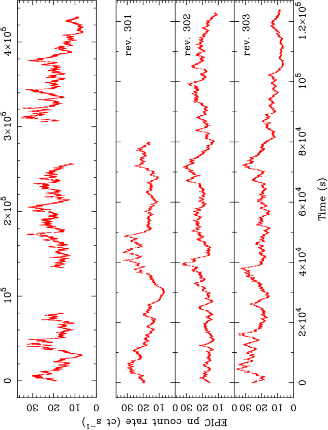
Figure 1: Full-band (0.2–10.0 keV) EPIC pn light curves in 100 s bins. The top panel shows all three consecutive light curves and the bottom panels show the individual light curves from each XMM-Newton revolution.

The featureless EXOSAT PSDs of Seyfert 1s provided no such timescales. Such breaks must exist, however, or the total power would diverge at low frequencies (for PSD slopes $\alpha\geq 1$). Indeed, in recent years dedicated X-ray monitoring programmes with RXTE have revealed deviations from the power-law PSD in a few Seyfert 1 galaxies; at low frequencies the PSD breaks to a flatter slope (Edelson & Nandra 1999; Uttley, M^cHardy & Papadakis 2002; Markowitz et al. 2002). The timescale of this break frequency is consistent with the idea that the PSD of AGN and GBHCs are essentially the same, with the characteristic timescales scaling linearly with the black hole mass. Such a linear scaling of timescales with black hole mass might be expected if the characteristic timescales are related to e.g. a light-crossing timescale or an orbital timescale. This linear scaling also means that a 100 ks light curve of a Seyfert galaxy (such as presented here) is comparable to a $\mathrel{\hbox{\hbox to0.0pt{\hbox{\lower 4.0pt\hbox{$\sim$}}\hss}\hbox{$<$}}}1$ s light curve of Cyg X-1. On these timescales a bright Seyfert 1 galaxy provides many more photons (by more than two orders of magnitude) than the GBHC, i.e. Seyferts have a higher count rate per characteristic timescale. This means that intensive monitoring of Seyferts can provide a view of the very high frequency variations in accreting black holes that is difficult to access even in bright GBHCs.

Not only do AGN and GBHCs show similar PSDs, but they display other striking similarities in their X-ray timing properties. Uttley & M^cHardy (2001) showed that both X-ray binary and AGN light curves show a tight, linear correlation between flux and rms variability amplitude (see also Edelson et al. 2002). The variability properties of GBHCs such as Cyg X-1 are a function of photon energy. The PSD shape above the high frequency break is energy-dependent, with the harder energy bands showing flatter PSD slopes (e.g. Nowak et al. 1999a; Lin et al. 2000). In addition the variations between different bands are highly coherent (well correlated at each Fourier frequency) and show time delays, with variations at softer energies leading those at harder energies (Miyamoto & Kitamoto 1989; Cui et al. 1997; Nowak et al. 1999a). The magnitude of the time delay is frequency dependent, with the delay increasing at lower frequencies. To date these properties have only been measured in one AGN, NGC 7469 (Nandra & Papadakis 2001; Papadakis, Nandra & Kazanas 2001), and in this object the energy-dependence of the PSD slope, the coherence and time delay properties appeared remarkably similar to those seen in Cyg X-1. These similarities re-enforce the idea that the X-ray emission mechanisms are the same in GBHCs and AGN.

This paper presents a detailed analysis of the X-ray continuum variability of the bright, variable Seyfert 1 galaxy MCG–6-30-15 ($z=0.007749$) using a long XMM-Newton observation. The large collecting area, wide band-pass and long orbit ($\sim 2$ day) of XMM-Newton make it ideal for examining the high frequency ($\mathrel{\hbox{\hbox to0.0pt{\hbox{\lower 4.0pt\hbox{$\sim$}}\hss}\hbox{$>$}}}10^{-5}$ Hz) timing properties of Seyfert galaxies. The analysis concentrates on frequency domain (i.e. Fourier) time series analysis techniques, as these are used extensively in the analysis of GBHC data. The rest of this paper is organised as follows. In Section 2 the data reduction procedures are outlined. In Section 3 the basic properties of the light curves are discussed, followed by an analysis of the PSD in Section 4. Spectral variability is then examined in detail by measuring the coherence and time lags between different energy bands, as discussed in Section 5. As these analyses are relatively new to AGN studies we discuss the methodology in some detail. Finally, the implications of these results are discussed in Section 6 and some concluding remarks are given in Section 7.

2 Data Reduction

XMM-Newton (Jansen et al. 2001) observed MCG–6-30-15 over the period 2001 July 31 – 2001 August 5 (revolutions 301, 302 and 303), during which all instruments were operating nominally. Fabian et al. (2002) discuss details of the observation and basic data reduction. For the present paper the data were reprocessed entirely with the latest software (SAS v5.3.3) but the procedure followed that discussed in the previous paper (except that the extraction region was a circle of radius 35 arcsec for both MOS and pn).

Light curves were extracted from the EPIC pn data in four different energy bands: 0.2–10.0 keV (full band), 0.2-0.7 keV (soft band), 0.7-2.0 keV (medium band) and 2.0-10.0 keV (hard band). These were corrected for telemetry drop outs (less than 1 per cent of the total time), background subtracted and binned to 100 s time resolution. The errors on the light curves were calculated by propagating the Poisson noise. The light curves were not corrected for the $\sim 71$ per cent “live time” of the pn camera (Strüder et al. 2001), which is only a scaling factor. The EPIC MOS light curves were also examined, but these are essentially identical to the pn light curves except with lower signal-to-noise. Therefore, in the rest of this paper the analysis concentrates on the pn data, but the MOS data are used to confirm the pn results of Section 5. The full band light curves are shown in Fig. 1. The revolutions provided three uninterrupted light curves of 80, 123 and 124 ks duration.

As discussed in Fabian et al. (2002), BeppoSAX observed MCG–6-30-15 simultaneously with XMM-Newton, but these data are not used in the present paper. The LECS and MECS data cover approximately the same bandpass as the EPIC (but with lower signal to noise) and the higher energy PDS data (with a count rate $\sim 0.7$ ct s^-1) do not have sufficient statistics to determine the high energy variability properties accurately. In addition, analysis of the BeppoSAX data is complicated by the poor sampling of the light curves (due to repeated Earth occulatations and SAA passages), indeed the amount of “good” exposure time obtained for the PDS was $40$ ksec spread over a $>400$ ksec observing period.

3 Basic temporal properties

The source shows a factor of five variation between minimum and maximum flux (both occurring during revolution 303), and significant variability can be seen on timescales as short as $\sim 100$ s.

As a first measure of the variability amplitude the root mean square (rms) amplitude, in excess of Poisson noise, was calculated as

$$\sigma_{\rm rms}=\sqrt{S^{2}-\overline{\sigma_{\rm{err}}^{2}}},$$ (1)

where $S^{2}$ is the total variance of the light curve $x(t_{i})$ of length $N$ data points

$$S^{2}=\frac{1}{N-1}\sum_{i=1}^{N}(x(t_{i})-\bar{x})^{2},$$ (2)

where $\bar{x}$ is the mean of $x(t_{i})$ and $\overline{\sigma_{\rm{err}}^{2}}$ is the contribution expected from measurement errors

$$\overline{\sigma_{\rm{err}}^{2}}=\frac{1}{N}\sum_{i=1}^{N}\left[\sigma_{{\rm err}}(t_{i})\right]^{2},$$ (3)

and $\sigma_{{\rm err}}(t_{i})$ is the error on $x(t_{i})$.

The fractional excess rms variability amplitude ($F_{\rm var}=\sigma_{\rm rms}/\bar{x}$; Edelson et al. 2002) and mean count rate ($\bar{x}$) were calculated for each of the three revolutions and are tabulated in Table 1. The errors on $F_{\rm var}$ were estimated using the prescription given by Edelson et al. (2002; but see their appendix A for caveats on the interpretation of these estimates). The medium band showed the highest variability amplitude. This can also been seen in Fig. 6 of Fabian et al. (2002), where the fractional rms spectrum peaked in the 0.7–2.0 keV band.

Table 1: Mean count rates ($\bar{x}$) and fractional excess rms variability amplitudes ($F_{\rm var}$) for the light curves from each revolution and in each energy band.

Revolution	band	$\bar{x}$ (ct s-1)	$F_{\rm var}$ (%)
301	Full	$18.51$	$28.7\pm 0.7$
	Soft	$8.63$	$27.8\pm 0.7$
	Medium	$6.68$	$32.3\pm 0.8$
	Hard	$3.27$	$26.0\pm 0.7$
302	Full	$19.94$	$19.3\pm 0.4$
	Soft	$8.85$	$18.4\pm 0.4$
	Medium	$7.53$	$21.4\pm 0.4$
	Hard	$3.61$	$19.3\pm 0.4$
303	Full	$18.41$	$34.9\pm 0.7$
	Soft	$8.56$	$31.8\pm 0.6$
	Medium	$6.69$	$40.1\pm 0.8$
	Hard	$3.22$	$33.7\pm 0.7$

3.1 Radiative efficiency

Fig. 2 shows a rapid “event” from the revolution 302 light curve. During this the source changed in 0.2–10 keV luminosity by $\Delta L\approx 1.5\times 10^{42}$ erg s^-1 in 100 s. This was used to estimate the radiative efficiency $\eta$ of the source, assuming photon diffusion through a spherical mass of accreting matter: $\Delta L/\Delta t\mathrel{\hbox{\hbox to0.0pt{\hbox{\lower 4.0pt\hbox{$\sim$}}\hss}\hbox{$<$}}}\eta\cdot 2.1\times 10^{42}$ erg s^-2 (Fabian 1979; Brandt et al. 1999). This gave a limit of $\eta\mathrel{\hbox{\hbox to0.0pt{\hbox{\lower 4.0pt\hbox{$\sim$}}\hss}\hbox{$>$}}}0.7$ per cent, below the expected maximum for accretion onto a black hole (6 and 30 per cent for non-rotating and maximally rotating black holes, respectively; Thorne 1974).

Figure 2: Section of the full-band (0.2–10.0 keV) EPIC pn light curve (from rev. 302) showing a rapid “flare” event.

3.2 rms-flux correlation

Using the 100 s resolution light curves the mean count rate and $\sigma_{\rm rms}$ were calculated in bins of 15 data points. The values of $\sigma_{\rm rms}$ from all three orbits were then binned as a function of count rate such that there were 20 measurements per bin, and an error was assigned based on the scatter within each bin (equation 4.14 of Bevington & Robinson 1992). Fig. 3 shows the resulting correlation between $\sigma_{\rm rms}$ and count rate in the four energy bands. The significance of the correlation was tested using the Spearman rank-order correlation coefficient, $r_{s}$, and the Kendall $\tau$ coefficient (Press et al. 1992). Both these indicate that the correlation is significant at $\mathrel{\hbox{\hbox to0.0pt{\hbox{\lower 4.0pt\hbox{$\sim$}}\hss}\hbox{$>$}}}99.5$ per cent confidence in all energy bands. The effect of the rms-flux correlation can be seen in the light curves (Fig. 1): the peaks of the light curves appear more variable (“jagged”) while the troughs appear much smoother.

Table 2 shows the results of fitting a linear model to these data; in all cases the linear model gives a good fit to the data, with a $y$-axis intercept consistent with zero. The gradient of this relation corresponds to the $F_{\rm var}$ measured only on these timescales (between 100 and 1500 s). The $1\sigma$ upper limit on any constant flux offset ($x$-intercept) is $1.2$ ct s^-1 for the full band, or $6.2$ per cent of the total count rate in that band. In the three energy sub-bands the upper limits on the constant flux offset are as follows: $1.04$ ct s^-1 ($12$ per cent), $0.09$ ct s^-1 ($1.3$ per cent) and $0.43$ ct s^-1 ($12.8$ per cent) for the soft, medium and hard bands respectively.

Table 2: Results of fitting a linear function to the rms-flux correlation. Errors on the model parameters correspond to a 90 per cent confidence level for one interesting parameter (i.e. a $\Delta\chi^{2}=2.7$ criterion).

Band	$y$-intercept	Gradient	$\chi^{2}/dof$
Full	$0.07\pm 0.22$	$0.052\pm 0.013$	$10.66/10$
Soft	$0.02\pm 0.12$	$0.049\pm 0.015$	$7.78/10$
Medium	$0.04\pm 0.07$	$0.057\pm 0.016$	$6.97/10$
Hard	$0.001\pm 0.049$	$0.065\pm 0.016$	$6.68/10$

4 Power spectral properties

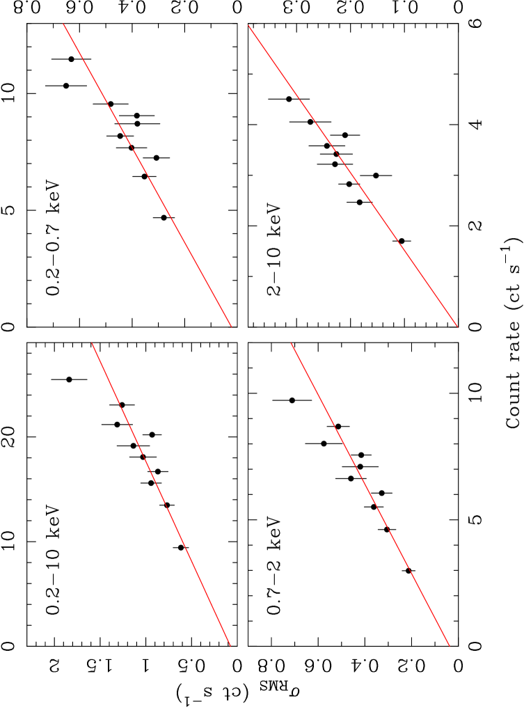
Figure 3: Correlation between rms variability amplitude and flux.

4.1 Estimating the power spectrum

The PSD (sometimes known as the auto spectrum) describes the amount of variability “power” as a function of Fourier frequency. The PSD and auto correlation function (ACF) are Fourier pairs, i.e. they are Fourier transforms of one another. For a general introduction to Fourier methods of time series analysis see e.g. Priestley (1981) and Bloomfield (2000), and for a review of Fourier techniques as applied to X-ray time series analysis see van der Klis (1989).

4.1.1 Measuring the periodogram

If the light curve $x(t_{i})$ is evenly sampled (with a sampling period $\Delta T$) then the PSD can be estimated by calculating the periodogram. This is the normalised, modulus-squared of the Discrete Fourier Transform (DFT) of the data. The DFT of the light curve, $X(f_{j})$, is calculated as (see Press et al. 1992):

$$X(f_{j})=\left(\frac{\Delta T}{N}\right)^{1/2}\sum_{i=1}^{N}x(t_{i})~{}\mathrm{e}^{2\mathrm{\pi}\mathrm{i}f_{j}t_{i}}=R_{X}(f_{j})+\mathrm{i}I_{X}(f_{j}),$$ (4)

where $R_{X}(f_{j})$ and $I_{X}(f_{j})$ are the real and imaginary parts of the DFT given by the discrete cosine and sine transforms, respectively:

$$R_{X}(f_{j})=\left(\frac{\Delta T}{N}\right)^{1/2}\sum_{i=1}^{N}x(t_{i})~{}\cos(2\mathrm{\pi}f_{j}t_{i})$$

$$I_{X}(f_{j})=\left(\frac{\Delta T}{N}\right)^{1/2}\sum_{i=1}^{N}x(t_{i})~{}\sin(2\mathrm{\pi}f_{j}t_{i}).$$ (5)

The transforms are normalised by $(\Delta T/N)^{1/2}$ so that the amplitudes are independent of the sampling and length of the light curve. The DFT is calculated at $N/2$ evenly spaced frequencies $f_{j}=j/N\Delta T$ (where $j=1,2,\ldots,N/2$). Thus the highest frequency accessible to the DFT is the Nyquist frequency, $f_{\rm Nyq}=f_{N/2}=1/2\Delta T$, and the lowest frequency is $f_{1}=1/N\Delta T$. Note that it is customary to subtract the mean flux from the light curve before calculating the DFT, this eliminates the zero-frequency power.

The complex valued DFT is then squared

$$|X(f_{j})|^{2}=X^{\ast}(f_{j})X(f_{j})=\{R_{X}(f_{j})\}^{2}+\{I_{X}(f_{j})\}^{2},$$ (6)

where ^∗ denotes the complex conjugate. The periodogram, $P(f_{j})$, is then calculated by choosing an appropriate normalisation:

$$P(f_{j})=\frac{2}{\bar{x}^{2}}|X(f_{j})|^{2}.$$ (7)

(Note that the Fourier transform has already been normalised in equations 4 and 4.1.1 to account for the data sampling.)

This normalisation (defined in van der Klis 1997, see also Miyamoto et al. 1991) is most commonly used in analysis of AGN and X-ray binaries because the integrated periodogram yields the fractional variance of the data (i.e. $F_{\rm var}^{2}$). This normalisation will be used throughout this paper. The factor of two is because this is a “one sided” normalisation; the periodogram is defined for both negative and positive frequencies, with this normalisation the integral over only positive frequencies yields the fractional variance. The integrated periodogram between two frequencies, say $f_{1}$ and $f_{2}$, yields the contribution to the fractional variance due to variations between the corresponding timescales $1/f_{2}$ and $1/f_{1}$ (this follows from Parseval’s theorem, see e.g. van der Klis 1989). The units for the periodogram ordinate are (rms/mean)² Hz^-1 (where rms/mean is the dimensionless quantity $F_{\rm var}$), or simply Hz^-1.

4.1.2 Poisson noise

If the time series is a continuous photon counting signal binned into intervals of $\Delta T$, as it is here, the effect of Poisson noise is to add an approximately constant amount of power to the periodogram at all frequencies. Thus, at high frequencies, where the red noise spectrum of the AGN is weak, the observed periodogram will be dominated by the flat (“white”) Poisson noise spectrum. With the above normalisation this constant Poisson noise level is $P_{N}=2/\bar{x}$. This formally assumes zero background flux, but for the present observation this is a reasonable approximation (even in the hard band the background count rate is $\sim 0.6$ per cent that of the source).

4.1.3 Scatter in the periodogram

A periodogram measured from a single light curve shows a great deal of scatter around the underlying PSD. This is a natural outcome of measuring the periodogram from a single realisation of a stochastic process. The result of this is that the periodogram at a given frequency, $P(f)$, is scattered around the underlying PSD, $\mathcal{P}(f)$, following a $\chi^{2}$ distribution with two degrees of freedom (see Section 6.2 of Priestley 1981):

$$P(f)=\mathcal{P}(f)\chi_{2}^{2}/2,$$ (8)

where $\chi_{2}^{2}$ is a random variable distributed as $\chi^{2}$ with two degrees of freedom, i.e. an exponential distribution with a mean and variance of two and four, respectively. The expectation value of the periodogram at a frequency $f$ is thus equal to the PSD but so is its standard deviation, as a result the periodogram shows a great deal of scatter. This fundamental property of the periodogram is discussed terms of X-ray time series analysis by e.g. Leahy et al. (1983), van der Klis (1989), Papadakis & Lawrence (1993), Timmer & König (1995) and Stella et al. (1997). In addition the periodogram is an inconsistent estimator of the PSD because this intrinsic scatter does not decrease as the number of data points in the light curve is increased. The periodogram can, however, be averaged (binned over separate light curves or adjacent frequencies) to reduce this scatter and produce a consistent estimate of the PSD (Jenkins & Watts 1968).

In GBHC analysis the light curves are typically broken into many separate segments and periodograms are calculated for each segment. At a given Fourier frequency the periodogram estimates from each light curve are identically and independently distributed (assuming the variability is stationary) and so their average will become Gaussian (following the central limit theorem). Therefore, averaging the periodograms from many independent light curve segments will produce a consistent estimate of the PSD with Gaussian errors (e.g. van der Klis 1997). However, dividing up the light curve limits the lowest frequency probed by the periodogram and so is not so suitable for AGN analysis where it is crucial to examine the widest frequency range possible.

An alternative technique is discussed by Papadakis & Lawrence (1993) and is in some sense “optimal” for red-noise light curves such as those from AGN. In this method a single periodogram is computed from the light curve, reaching down to the lowest accessible frequencies, and periodogram estimates at consecutive frequencies are averaged. For evenly sampled data the periodogram estimates at each Fourier frequency are independently distributed (according to equation 8) and so the averaged periodogram estimate in each frequency bin will tend to a Gaussian distribution. In the method of Papadakis & Lawrence (1993) it is the logarithm of the periodogram that is binned, such that each bin contains $N\geq 20$ periodogram estimates, and an error is assigned based on the scatter within each bin. Using the logarithm of the periodogram means the distribution of the binned periodogram converges on Gaussian with fewer data points per bin, and therefore allows for finer frequency binning. This binning method is used throughout this paper to produce binned periodogram estimates with errors. (See also van der Klis 1997 for more on binned periodogram estimates.)

4.1.4 Bias in the periodogram

A further point is that periodograms measured from finite data tend to be biased by windowing effects which further complicate their interpretation (van der Klis 1989; Papadakis & Lawrence 1993; Uttley et al. 2002). The observed light curve ($f(t)$) is the true, continuous light curve of the source ($l(t)$) multiplied by the sampling, “window,” function ($w(t)$):

$$f(t)=l(t)\cdot w(t),$$ (9)

where the window function takes the value unity when the light curve is sampled and zero elsewhere. From the convolution theorem of Fourier transforms, the Fourier transform of the observed light curve ($F(f)$) is the Fourier transform of the true light curve ($L(f)$) convolved with the Fourier transform of the window function ($W(f)$):

$$F(f)=L(f)\otimes W(f).$$ (10)

The periodogram (which is the square of the discrete Fourier transform of the observed light curve) is therefore the periodogram of the continuous light curve of the source multiplied by the periodogram of the window function. Thus the periodogram distorted away from the true PSD by the sampling, i.e. the convolution with the spectral window function.

This leads to two main effects. The first is due to the discrete sampling of the data. If the light curve is not contiguously sampled then power from frequencies above the Nyquist frequency can be folded back, or “aliased,” into the observed frequency range. For binned, continuous light curves such as those presented here, the aliasing will negligible (see van der Klis 1989). In any event, from continuous data the very high frequency spectrum will dominated by the Poisson noise level and not aliasing.

The second effect is “red noise leak” and arises as a result of the finite duration of the light curve. Power is transferred from low to high frequencies by the lobes of the spectral window function (see e.g. Deeter & Boynton 1982; van der Klis 1997). If there is significant power at frequencies below the lowest frequency probed by the periodogram (i.e. on timescales longer than the length of the observation), this can manifest itself as slow rising or falling trends across the light curve. These trends will contribute to the total variance of the light curve (and thus the total power) but, as the periodogram does not extend to such low frequencies, the power will be transfered into the observed frequency band-pass (i.e. it will “leak” to higher frequencies). Red noise leak tends to add a constant component to the observed periodogram in the form of a power-law of slope $\alpha=2$ (i.e. the PSD of a linear trend; see van der Klis 1997 for more details), the amplitude of this depends on the PSD of the source at low frequencies (see also section 3.3 of Papadakis & Lawrence 1995). The effect of red noise leak on the periodogram can be accounted for using the Monte Carlo simulation procedure outlined below.

4.2 PSD fitting procedure

The method employed in the present work is similar to the methods discussed by Done et al. (1992), Green, M^cHardy & Done (1999) and Uttley et al. (2002). A model PSD is assumed, multiple realisations (light curves) are simulated using this PSD and are resampled to match the original data (thereby including the distorting effects of the sampling). Periodograms are then calculated from the simulated light curves in the same manner as the real data, averaged over the realisations, and this “average distorted model” (ADM), which includes the effects of red noise leak, is compared to the original periodogram using a goodness-of-fit measure. This method therefore accounts for the biases in the periodogram introduced by the window function. It is important to bear in mind that, as with any model-fitting procedure, the results depend on the assumptions made, i.e. the choice of specific models to test.

The errors derived from the periodograms (see Section 4.1.3) are approximately Gaussian (Papadakis & Lawrence 1993) and therefore the $\chi^{2}$ statistic can be used to estimate the goodness of the fit. Once a reasonable fit is found, uncertainties on the model parameters can be estimated using the $\Delta\chi^{2}$ criterion (e.g. Lampton, Margon and Bowyer 1976), as in X-ray energy spectrum fitting.

The algorithm described by Timmer & König (1995) was used to generate the simulated light curves from the model PSD. This algorithm generates a random time series from an arbitrary broad-band PSD, correctly accounting for the intrinsic scatter in the powers (i.e. equation 8), and is computationally very efficient. The effects of red noise leak can be accounted for by extending the PSD model to much lower frequencies than required, generating light curves much longer than the observed light curve and using only a segment of the required length. Data simulated in such a fashion will include power on timescales much longer than those probed by each segment alone.

The fitting procedure is as follows.

1. A model PSD is chosen and 500 random light curves are generated using the algorithm of Timmer & König (1995). The simulated light curves were $\approx 26$ times longer duration than the orbital light curves in order that red noise leak is accounted for.

2. From each of the simulated light curves a section from the middle is resampled to match the data. Specifically, from each (long) simulated light curve three consecutive light curves were extracted, to match the three consecutive revolutions, using exactly the same sampling as the real data. The logarithmically binned periodogram is computed in exactly the same way as for the real data (Section 4.3).

3. The 500 binned periodograms are then averaged to produce the ADM - this represents the periodogram after being distorted by the light curve sampling (folded through the window function).

4. The constant Poisson noise level is added and the comparison between the ADM and the data is then made by calculating the $\chi^{2}$ of the fit.

5. The normalisation of the ADM is then adjusted to minimise the $\chi^{2}$ (keeping the Poisson noise level fixed).

6. The $\chi^{2}$ of the fit is then evaluated over a grid of PSD models and the minimum, corresponding to the best-fitting model, is found.

This method differs slightly from the method of Uttley et al. (2002). Firstly, because the XMM-Newton light curves are continuous the effects of aliasing are negligible, thus the simulated light curves were generated with the same time resolution as the data (100 s). The sparsely sampled RXTE data used by Uttley et al. (2002) meant that aliasing was a significant factor and needed to be accounted for in the simulations. The second major difference is that Uttley et al. (2002) calculated errors on the ADM (based on the scatter in the simulated periodograms), and these were used to estimate the goodness of fit. In the present analysis there are enough data points to apply the Papadakis & Lawrence (1993) binning (with $N=20$) and estimate the error on the observed periodogram directly from the data, for use with $\chi^{2}$-fitting.

The $\chi^{2}$ fitting employed in this method relies on the data being binned sufficiently. It would in principle be possible to make use of the maximum frequency resolution offered by the unbinned periodogram by choosing a different goodness-of-fit estimator (e.g. deriving the rejection probability directly from the Monte Carlo trials, as in Uttley et al. 2002). However, the results (the best-fitting parameters) are model-dependent in any case and so using a different method is unlikely to yield any further information.

4.3 The periodogram of MCG–6-30-15

The periodogram of the full-band data was computed by calculating the periodogram for each revolution of data (following equation 7). The light curves from each revolution, when taken separately, are perfectly evenly sampled and uninterrupted. This means that for each light curve the periodogram estimates are independent at each Fourier frequency, and they are also independent between the periodograms from the three light curves. The periodograms for the three light curves were therefore combined to produce a single, binned periodogram by sorting the periodogram points by frequency and then applying the logarithmic binning (Papadakis & Lawrence 1993).

Furthermore, no additional windowing was applied to the data (see Section 13.4 of Press et al. 1992 and section 7.5 of Priestley 1981). Windowing is often used to suppress the leak of power from one frequency to another, as it suppresses the side-lobes of the spectral window function $W(f)$ and therefore the amount of power displaced to distant frequency bins. However, in exchange for this the central lobe of the spectral window function is broadened, meaning more power is lost to neighbouring frequency bins. This transfer of power between consecutive frequency bins means they are no longer independently distributed, which is required by the binning method applied above.

In order to accurately estimate the Poisson noise level, the periodograms were first calculated using the full-band light curves with 10 s resolution. This allows the periodogram to extend up to high frequencies, at which the variability is dominated by Poisson noise. Fig. 4 shows the periodograms from each of the three orbits (binned by $N=50$) and the combined periodogram (binned by $N=100$ to improve the signal-to-noise). The red noise PSD of the source can be seen below $\sim 3\times 10^{-3}$ Hz, above which the (white) Poisson noise spectrum dominates. Also marked are the predicted noise levels assuming just Poisson noise in the data. These show that the predicted noise level is clearly an accurate estimate of the true noise level in the data. In the following analysis only the 100 s resolution light curves are used, since above the Nyquist frequency ($5\times 10^{-3}$ Hz) the periodogram is dominated by the Poisson noise and not the source variability, and the Poisson noise level is assumed to be at the expected value.

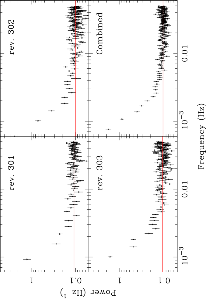
Figure 4: High frequency periodograms estimated using 10 s resolution, full-band light curves. At high frequencies the periodograms are dominated by the flat (white) Poisson noise spectrum. The solid lines show the expected Poisson noise levels.

Fig. 5 shows the raw periodograms (binned by $N=20$), calculated by combining the periodograms from each revolution. The red noise PSD of the source is clearly detected above the Poisson noise level at frequencies below $\sim$few $10^{-3}$ Hz in all bands. In the following sections these “dirty” periodograms were fitted using the Monte Carlo procedure in order to derive the properties of the PSD in a robust manner.

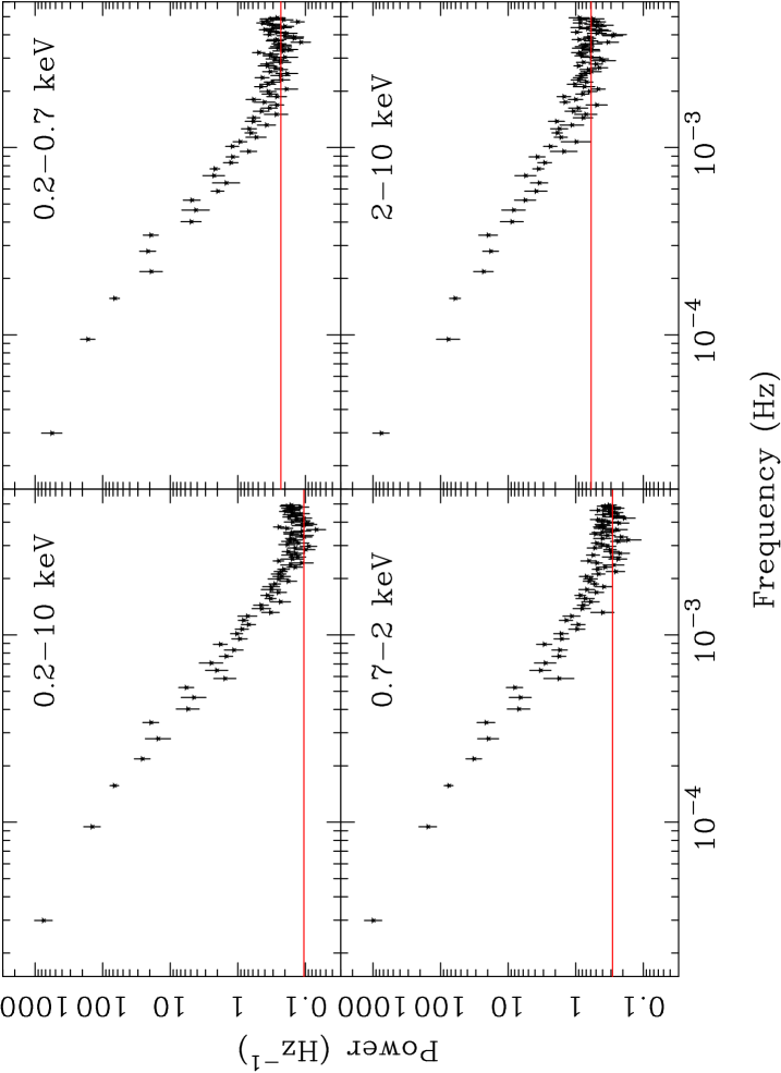
Figure 5: Periodograms for each energy band calculated using three revolutions of data. The solid lines show the expected Poisson noise levels.

4.4 Results

4.4.1 The full-band PSD of MCG–6-30-15

Table 3: Results of fitting the full-band periodogram with various trial models. The models are discussed in the text and shown in Fig. 6. Model 1 is a simple power-law, model 2 is a power-law breaking to a slope of $\alpha_{\rm low}=1$ at low frequencies, model 3 is a power-law with a break to $\alpha_{\rm low}=0$, model 4 is a power-law with a smooth transition to a slope of $\alpha_{\rm low}=1$ at low frequencies and model 5 is an exponentially cut-off power-law. Errors on the model parameters correspond to a 90 per cent confidence level for one interesting parameter (i.e. a $\Delta\chi^{2}=2.7$ criterion).

Model	Slope $\alpha$	Break freq. $f_{\rm br}$ ($10^{-5}$ Hz)	$\chi^{2}/dof$
1	2.10	—	$160.8/79$
2	$2.50\pm 0.15$	$10_{-4}^{+10}$	$87.2/78$
3	$2.45\pm 0.15$	$5_{-1}^{+3}$	$89.0/78$
4	$2.65\pm 0.20$	$13_{-6}^{+8}$	$84.1/78$
5	$1.8\pm 0.1$	$100\pm 30$	$83.4/78$

As expected, the periodograms shown in Fig. 5 show an approximately power-law spectrum for the intrinsic (source) variability. Various trial models were fitted to the data (the models are illustrated in Fig. 6), using the procedure outlined above to constrain the PSD. The first trial model was a power-law (model 1):

$$\mathcal{P}(f)=Nf^{-\alpha}.$$ (11)

This model has two free parameters, namely the slope ($\alpha$) and normalisation ($N$) of the power-law (the additional constant Poisson noise level, $P_{N}$, is kept fixed). As summarised in Table 3, this model provided an unacceptable fit to the data ($>99.99$ per cent rejection probability). Fig. 7 shows the variation in $\chi^{2}$ with $\alpha$ (for 79 degrees of freedom, $dof$). The $\chi^{2}$ of the fit changes little for PSD slopes steeper than $2$. This is an effect of the red noise leak. If the PSD continues to very low frequencies as a steep power-law ($\alpha>2$), a significant amount of power will leak into the observed periodogram in the form of an $\alpha=2$ power-law. This red noise leak contribution will cause the observed periodogram to have a slope of $\alpha\approx 2$ even when the true underlying PSD slope is much steeper. Thus, if the power-law PSD continues unbroken to low frequencies, it is difficult to distinguish slopes steeper than $2$ in the fitting.

Figure 6: Trial PSD models used to fit the full-band data.

Figure 7: Fit statistic against power-law index for a simple power-law PSD model (model 1, with $79~{}dof$).

Figure 8: The full-band data (points with errors) and best-fitting single power-law model (model 1; solid line). The residuals from the fit are shown in the lower panel.

Fig. 8 shows the best fitting power-law model, with a slope of $\alpha=2.1$. This steep slope implies that the PSD must break at low frequencies or the integrated power would diverge. Therefore PSD models including a flattening at low frequencies were explored in an attempt to constrain the frequency of the break. The residuals from the power-law fit show that the model is too flat above $2\times 10^{-4}$ Hz and too steep at lower frequencies, suggesting the PSD may break in the observed frequency range.

Indeed, based on long timescale RXTE monitoring, Uttley et al. (2002) found the best fitting PSD model for MCG–6-30-15, in the 2–10 keV band, was a broken power-law. When the slope below the break was fixed at $\alpha_{\rm low}=1$ the slope above the break was found to be $\alpha=2.0\pm 0.3$, with a break frequency in the range $1.3\times 10^{-5}$ to $1.0\times 10^{-4}$ Hz (90 per cent confidence limits). Therefore the next trial model fitted was a broken power-law (model 2)

$$\mathcal{P}(f)=\left\{\begin{array}[]{l@{\quad:\quad}l}N\left(\frac{f}{f_{\rm br}}\right)^{-\alpha_{\rm low}}&f\leq f_{\rm br}\\ N\left(\frac{f}{f_{\rm br}}\right)^{-\alpha}&f>f_{\rm br},\end{array}\right.$$ (12)

with a break from a slope of $\alpha_{\rm low}=1$ to $\alpha$. The free parameters were the high frequency slope ($\alpha$), the normalisation ($N$), and the frequency of the break ($f_{\rm br}$). The fit parameters are given in Table 3. The model provided an acceptable fit to the data (77 per cent rejection probability) and the improvement in the fit was $\Delta\chi^{2}=73.6$ for the addition of one free parameter (the break frequency), which, according to the $F$-test, is significant at $>99.99$ per cent confidence. Fig. 10 shows the confidence contours for the model parameters and the fit residuals using this model are shown in Fig. 9.

Figure 9: The full-band data and (folded) broken power-law model (model 2).

Although there are only two periodogram points at frequencies below the break, the detection of the break is nevertheless highly significant. This is because the high frequency PSD slope is observed to be steeper than $2$, implying that the effect of red noise leak is not strong. The steep PSD observed at high frequencies cannot continue below the lowest observed frequencies; if the PSD remained steep to low frequencies the contribution from red noise leak would cause the periodogram to resemble a $\alpha=2$ power-law over the whole observed frequency range. The steep PSD at high frequencies must therefore break to a flatter slope close to the lowest frequencies probed in order that the high frequency periodogram have a steep slope.

Figure 10: Contour plot showing the parameters of model 2. The contours represent 68.3, 90 and 99 per cent confidence levels.

The slope of the PSD below the break is not well-constrained from the XMM-Newton data however. Fitting the data with a PSD model that breaks from a slope of $\alpha_{\rm low}=0$ (model 3) gives a similarly acceptable fit but with a slightly lower break frequency (Table 3, Fig. 11). As these two models both give good fits it is not possible to distinguish between them based on these data alone. However, it is interesting to note that the break frequency found from the RXTE data is consistent with the break frequency found from the XMM-Newton data when the PSD is assumed to break to $\alpha_{\rm low}=1$. The break frequencies found from fitting the model assuming a break to $\alpha_{\rm low}=0$ are inconsistent between RXTE ($f_{\rm br}=5.1_{-2.6}^{+5.1}\times 10^{-6}$ Hz) and XMM-Newton ($f_{\rm br}=5_{-1}^{+3}\times 10^{-5}$ Hz).

Figure 11: As Fig. 10 except for model 3.

The exact shape of the break is not well defined from these data. As an alternative to a sharply broken power-law, a model representing a power-law with a smooth break from a slope of $\alpha_{\rm low}=1$ to $\alpha$ was tested (model 4):

$$\mathcal{P}(f)=Nf^{-1}\left\{1+\left(\frac{f}{f_{\rm br}}\right)^{2}\right\}^{-(\alpha-1)/2}.$$ (13)

This has three free parameters, $N$, $\alpha$ and $f_{\rm br}$, and provided an acceptable fit (Table 3, Fig. 12), comparable to the models including a sharp break, and the break frequency was consistent with that found for model 2.

Figure 12: As Fig. 10 except for model 4

The final model tested was an exponentially cut-off power-law (model 5):

$$\mathcal{P}(f)=Nf^{-\alpha}\mathrm{e}^{-(f/f_{\rm br})^{2}}$$ (14)

Again this model has three free parameters, $N$, $\alpha$ and $f_{\rm br}$, and provided a reasonable fit to the data (Table 3, Fig. 13). The best-fitting slope for this model is much flatter than for the previous models, and the cut-off frequency is much higher than the break frequencies in the broken power-law models. That this model provides a good fit to the data is perhaps suggesting that the PSD of MCG–6-30-15 steepens further at high frequencies.

Figure 13: As Fig. 10 except for model 5

4.4.2 Energy dependence of the PSD

On the basis of the XMM-Newton data alone, PSD models 2 through 5 all provide reasonable fits to the full-band data. In the following analysis, model 2 is fitted to the data from the soft, medium and hard energy bands. in order to provide a uniform parameterisation of the PSD at different energies. The residuals are shown in Fig. 14 and the results from these fits are shown in Fig. 15 and Table 4.

The fits to the soft and hard band data using model 2 are somewhat worse than the fit to the full band data. However, as can been seen from Fig. 14, there are no obvious, strong, systematic residuals. Refitting these data with model 4 provided very similar fits and refitting using model 5 gave a slightly better fit to the hard band data but slightly worse fits to the soft and medium bands. The possibility remains that there is some marginally significant structure in the PSDs at high frequencies (around $\sim 4\times 10^{-3}$ Hz in Fig. 14), not accounted for in these simple continuum models, as was also suggested for the high frequency PSD of NGC 7469 by Nandra & Papadakis (2001). These points notwithstanding, model 2 was used to parameterise, in a simple and uniform fashion, the PSD as a function of energy.

The break frequencies as determined in each energy band are consistent with one another. However, the slope of the PSD above the break shows significant changes between the energy bands, with the hardest band showing the flattest slope. Table 4 also gives the total variability powers, in $F_{\rm var}$ form, derived from each band (cf. Table 1). For each band the total power was estimated by integrating binned periodogram (after subtracting off the constant Poisson noise level) to give $F_{\rm var,1}$, and also by integrating the PSD model (excluding the Poisson noise component) over the frequency range $10^{-5}$ to $5\times 10^{-3}$ Hz to give $F_{\rm var,2}$. As was noted in Section 3, the medium band contains the highest total variability power.

Figure 14: Residuals from fits to the soft, medium and hard band data using the broken power-law model (model 2).

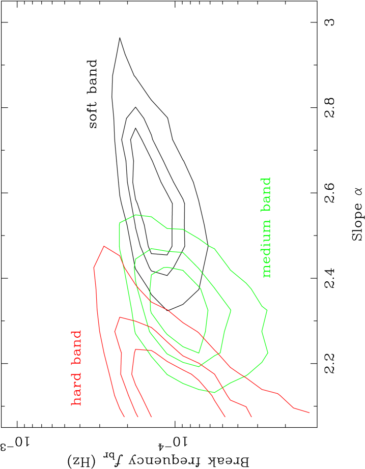
Figure 15: Contour plot showing the parameters of the broken power-law model (assuming a slope of $\alpha_{\rm low}=1$ below the break) for the three energy sub-bands. The contours represent 68.3, 90 and 99 per cent confidence levels.

Table 4: Results of fitting the periodograms derived from the four energy bands with the broken power-law model (breaking from a slope of $\alpha$ to slope of $\alpha_{\rm low}=1$ at low frequencies). Errors on the model parameters correspond to a 90 per cent confidence level for one interesting parameter (i.e. a $\Delta\chi^{2}=2.7$ criterion). Also given are the total powers calculated by integrating the binned periodogram ($F_{\rm var,1}$) and by integrating the best-fitting PSD model ($F_{\rm var,2}$).

	Slope	$f_{\rm br}$		$F_{\rm var,1}$	$F_{\rm var,2}$
Band	$\alpha$	($10^{-4}$ Hz)	$\chi^{2}/dof$	(%)	(%)
full	$2.50\pm 0.15$	$10_{-4}^{+10}$	$87.2/78$	26.0	26.3
soft	$2.55\pm 0.20$	$13_{-5}^{+7}$	$108.4/78$	23.8	23.8
medium	$2.30\pm 0.15$	$8_{-3}^{+8}$	$89.2/78$	29.3	29.1
hard	$2.10\pm 0.15$	$10_{-6}^{+10}$	$103.5/78$	25.4	24.0

4.4.3 Low frequency PSD

The binned periodograms used above reached down to $3\times 10^{-5}$ Hz in the lowest frequency bin. It would in principle be possible to treat the three consecutive light curves as a single, longer light curve (top panel of Fig. 1) and use this to reach even lower frequencies in the power spectrum. However, this three revolution light curve is no longer uninterrupted, due to the gaps between revolutions. This means that the standard DFT (as discussed in Section 4.1.1) is no longer suitable. There do exist periodogram estimators designed to deal with data containing gaps, such as the Lomb-Scargle periodogram (Lomb 1976; Scargle 1982) but there are drawbacks to using such techniques. Firstly, the gaps in the sampling mean the periodogram estimates at each frequency are no longer independent of one another (Scargle 1982), so the binning and error estimation used above is not strictly valid. Secondly, the more complicated window function introduces much greater distortion on the low frequency periodogram, which would severely limit the amount of information that could be recovered from the lowest frequencies. For these reasons the results presented in this paper are based entirely on the more robust, standard DFT method, but for completeness the Lomb-Scargle periodogram (computed using the algorithm of Press & Rybicki 1989) of the full-band light curve is shown in Fig. 16. Down to low frequencies this appears broadly consistent with the results presented above.

Figure 16: Unbinned Lomb-Scargle periodogram of the full-band light curve. The large scatter in the periodogram is expected (see Section 4.1.3). The dashed line illustrates the broken power-law model used in Section 4.4. Note that the model has not been fitted to the data and that the Lomb-Scargle periodogram is normalised differently from the periodogram discussed in Section 4.1.1.

4.4.4 Stationarity

The fundamental assumption underpinning the above analysis is that the variability process is stationary. A stationary process is one whose statistical properties do not depend on time (see section 1.3 of Bendat & Piersol 1986 for more on stationarity in random data). Specifically, the assumption made here is that the PSD is stationary, i.e. that the light curves are all realisations of the same process. The rms-flux correlation found in Section 3.2 shows that the variability of MCG–6-30-15 is in some sense non-stationary (the variance does change), but in a “well-behaved” fashion. Indeed, the linear correlation between $\sigma_{\rm rms}$ and $\bar{x}$ means that the average $F_{\rm var}$ is constant. In other words, the variations, when normalised by the local flux, appear stationary.

The method outlined in Appendix A of Papadakis & Lawrence (1995) was used as a simple check of the validity of this assumption. If the PSD $\mathcal{P}(f)$ is constant then the (unbinned) periodograms obtained from each revolution should be identical except for the scatter dictated by equation 8. Papadakis & Lawrence (1995) define the statistic $S$ from the logarithm of the ratio of two periodograms, summed over a range of frequencies.

$$S=\frac{1}{\sqrt{N}}\sum_{i=1}^{N}\frac{\log[P_{1}(f_{i})]-\log[P_{2}(f_{i})]}{\sqrt{{\rm var}\{\log[P_{1}(f_{i})]\}+{\rm var}\{\log[P_{2}(f_{i})]\}}},$$ (15)

where $P_{1}(f_{i})$ and $P_{2}(f_{i})$ are the two periodograms, and ${\rm var}\{\log[P_{1,2}(f_{i})]\}=0.31$ (Papadakis & Lawrence 1993).

If the underlying PSD is the same in the two periodograms then $S$ should be normally distributed with a mean of zero and a variance of unity.

A normalised periodogram was computed for the first 80 ksec of each of the three revolutions (the light curves were clipped to equal duration so that their periodograms had identical Fourier frequencies) and $S$ was measured for frequencies below $10^{-3}$ Hz, where the source variability dominates over the Poisson noise. Comparing rev. 301 and 302 gave $S=1.18$, comparing rev. 301 and 303 gave $S=-0.26$ and comparing rev. 302 and 303 gave $S=-1.44$. These three estimates are all within $2\sigma$ of the expected value assuming stationarity in the data. Therefore, to first-order at least, the assumption of stationarity in these data seems a reasonable one.

5 Cross spectral properties

5.1 The cross spectrum

The PSD is often called the auto spectrum because it is the Fourier transform of the light curve, multiplied by itself (equation 6). The cross spectrum is a related tool used for comparing the properties of two simultaneous light curves, such as from different energy bands, say $x(t)$ and $y(t)$. The product of the Fourier transforms of the two light curves gives the cross spectrum (compare with equation 6):

$$C(f)=X^{\ast}(f)Y(f).$$ (16)

In the same way that the PSD (auto spectrum) and the ACF are Fourier pairs, the cross spectrum and cross correlation function (CCF) are also Fourier pairs. Thus, mathematically speaking, the cross spectrum contains the same information as the CCF.

The cross spectrum is complex valued and can be represented in the complex plane by an amplitude and a phase. The complex Fourier transforms of the two light curves can be written as $X(f)=|X(f)|\mathrm{e}^{\mathrm{i}\phi_{x}(f)}$ and $Y(f)=|Y(f)|\mathrm{e}^{\mathrm{i}\phi_{y}(f)}$ and the cross spectrum can be written as:

$$C(f)=|X(f)||Y(f)|\mathrm{e}^{\mathrm{i}(\phi_{y}(f)-\phi_{x}(f))}.$$ (17)

The phase component of the cross spectrum represents the phase difference between the two light curves (which corresponds to a time delay at that frequency) and is discussed more fully in Section 5.3. The squared magnitude of the cross spectrum is used to define the “coherence” of the two light curves.

5.2 Coherence

5.2.1 The meaning of coherence

The coherence, $\gamma^{2}(f)$, is a real-valued function and is essentially the squared cross spectrum normalised by the auto spectra (PSDs) of the two light curves.

$$\gamma^{2}(f)=\frac{|\langle C(f)\rangle|^{2}}{\langle|X(f)|^{2}\rangle\langle|Y(f)|^{2}\rangle}.$$ (18)

Here the angled brackets represent an averaging over an ensemble of realisations of the processes. Coherence differs from the periodogram and time lags in the sense that it is only meaningful to talk of the coherence from an ensemble of independent measurements (either from separate light curve segments or consecutive frequencies). Equation 18 defines the linear correlation coefficient of $X(f)$ and $Y(f)$ (see Section 9.1 of Priestley 1981). The coherence can thus be thought of as a measure of the degree of linear correlation between the two light curves as a function of Fourier frequency, and is related to the amplitude of the CCF.

In order to illustrate coherence, consider two light curves that are related by a transfer function $\psi(\tau)$, e.g.

$$y(t)=\int_{-\infty}^{+\infty}\psi(t-\tau)x(\tau)d\tau=\psi(t)\otimes x(t).$$ (19)

Then from the convolution theorem

$$Y(f)=\Psi(f)X(f),$$ (20)

where $\Psi(f)$ is the Fourier transform of $\psi(t)$. Therefore:

$$|Y(f)|^{2}=Y^{\ast}(f)Y(f)=|\Psi(f)|^{2}|X(f)|^{2},$$ (21)

and

$$C(f)=X^{\ast}(f)Y(f)=X^{\ast}(f)\Psi(f)X(f)=\Psi(f)|X(f)|^{2}.$$ (22)

The squared magnitude of the cross spectrum then becomes:

$$|C(f)|^{2}=|X(f)|^{4}|\Psi(f)|^{2}.$$ (23)

And so

$$\frac{|C(f)|^{2}}{|X(f)|^{2}|Y(f)|^{2}}=\frac{|X(f)|^{4}|\Psi(f)|^{2}}{|X(f)|^{2}|\Psi(f)|^{2}|X(f)|^{2}}=1.$$ (24)

Therefore the coherence is $\gamma^{2}(f)=1$.

This means that if the two light curves are related by a single, linear transfer function (e.g. a delay or a smoothing) then they will have unity coherence. In other words, if knowledge of one light curve can in principle be used to predict the other, the two are said to be perfectly coherent. If, on the other hand, the light curves contain contributions from completely independent processes then the coherence will be less than unity.

Another way of thinking about coherence is in terms of equation 17. If the light curves are related by some simple transform then, at a frequency $f$, there will be a fixed delay between the light curves, i.e. the lag will be the same in each realisation of the process. If the phase difference is constant then the value of the numerator of equation 18 (the squared mean of equation 17) is equal to the denominator and hence the the coherence is unity. The interpretation of coherence is illustrated more fully in Vaughan & Nowak (1997) and Nowak et al. (1999a).

5.2.2 Estimating the coherence

In an analogous manner to the PSD, the cross spectrum is estimated using the cross periodogram. If the two discretely sampled light curves, $x(t_{i})$ and $y(t_{i})$, have DFTs $X(f_{j})$ and $Y(f_{j})$ then the cross periodogram is given by the discrete form of equation 16, namely:

$$C(f_{j})=X^{\ast}(f_{j})Y(f_{j})=R_{C}(f_{j})+\mathrm{i}I_{C}(f_{j}),$$ (25)

where $R_{C}(f_{j})$ and $I_{C}(f_{j})$ are the real and imaginary components of the complex cross spectrum:

$$R_{C}(f_{j})=R_{X}(f_{j})R_{Y}(f_{j})+I_{X}(f_{j})I_{Y}(f_{j})$$

$$I_{C}(f_{j})=R_{X}(f_{j})I_{Y}(f_{j})-I_{X}(f_{j})R_{Y}(f_{j}),$$ (26)

and $R_{X}(f_{j})$ and $I_{X}(f_{j})$ are the real and imaginary components of the DFT of the light curve $x(t_{i})$ as defined by equation 4.1.1. The coherence is estimated using the discrete form of equation 18:

$$\gamma^{2}(f_{j})=\frac{\langle R_{C}(f_{j})\rangle^{2}+\langle I_{C}(f_{j})\rangle^{2}}{\langle|X(f_{j})|^{2}\rangle\langle|Y(f_{j})|^{2}\rangle}.$$ (27)

The angled brackets here represent an averaging over light curve segments and/or consecutive frequencies. In practice however, the coherence will be compromised by photon noise, which is independent between the two light curves and so will lead to an apparently reduced coherence. As the Poisson noise power is known, this effect can be removed using the recipe outlined in Vaughan & Nowak (1997). In the following analysis the noise-corrected coherence and its uncertainty were estimated using equation 8 of Vaughan & Nowak (1997). The coherence was calculated only for frequencies below $10^{-3}$ Hz, above this frequency the Poisson noise power becomes comparable to the intrinsic source variability and equation 8 of Vaughan & Nowak (1997) becomes increasingly inaccurate.

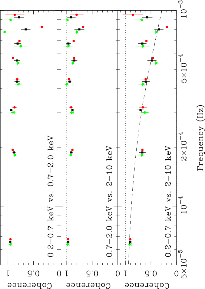
Figure 17: Coherence functions between light curves in the three energy bands. The different symbols mark the results derived using light curves from the three EPIC detectors (squares mark pn, circles mark MOS1 and stars mark MOS2 data). The dotted line shows the function $\gamma^{2}(f)=\exp(-f/8\times 10^{-4}~{}\rm{Hz})$ discussed in the text.

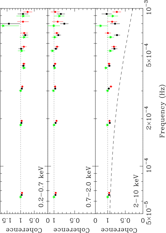
Figure 18: Coherence functions between light curves from different detectors in the same energy bands (squares mark pn vs. MOS1, circles mark pn vs. MOS2 and stars mark MOS1 vs. MOS2). As these were calculated between light curves from different detectors but identical energy ranges the intrinsic coherence is unity and deviations from unity are a result of Poisson noise. The dotted line shows the function plotted in Fig. 17 representing the loss of coherence observed between the energy bands. Clearly this function shows a much more pronounced loss of coherence than that resulting from Poisson noise.

As mentioned above, the coherence needs to be averaged in some fashion. For the present analysis the cross and auto spectra were calculated separately for each revolution. The data from the three revolutions were then combined by sorting in order of frequency and then averaged in bins of $N=40$ frequency points.

5.2.3 Coherence properties of MCG–6-30-15

The coherence function was calculated for the three possible combinations of the three energy bands (soft/medium, soft/hard and medium/hard). This was repeated using data from MOS1 and MOS2 as well as the pn and the results were consistent between the detectors. (The coherence was also estimated individually for each revolution of data and the results were consistent between the three revolutions.) The resulting coherence functions are shown in Fig. 17. At low frequencies the coherence is close to unity for all energy bands. At higher frequencies the coherence becomes much lower, particularly between the soft and hard bands. For comparison, Fig. 17 shows the function $\gamma^{2}(f)=\exp(-f/8\times 10^{-4}~{}\rm{Hz})$ compared to the coherence between soft and hard bands.

This apparent loss of coherence at high frequencies could be an effect of Poisson noise in the data, since at high frequencies the intrinsic source power is weaker compared to the noise power. In order to test this possibility the coherence was evaluated by comparing light curves in identical energy ranges from the three different detectors. The light curves extracted from the three detectors should be identical, in a given energy band, except for Poisson noise. Therefore the coherence should be unity and any deviation from unity will be a result of Poisson noise. As can been seen from Fig. 18, the coherence is close to unity until the highest frequencies, and the deviation from unity coherence at high frequencies is much smaller than the observed loss of coherence between the different energy bands. This, and the fact that the loss of coherence is repeated in all three detectors suggests that Poisson noise is not seriously biasing these results, and that the error bars are reasonable estimates of the true uncertainties.

5.2.4 Simulations

Simulated data were used as an additional test of the accuracy of the coherence estimation. Two simulated light curves were constructed, representing light curves in two different bands, and the coherence was calculated for them exactly as for the real data. These simulations were used as a further test of the effect of Poisson noise and to measure the effect of different PSD slopes on the coherence function.

The effect of Poisson noise was tested by simulating coherent data in two bands using the same PSD. The PSD model used was taken from the fit to the soft band data using model 2 (Table 4). Two long light curves were generated using this PSD and an identical random number sequence. The two light curves, having identical PSDs as well as Fourier phases and amplitudes, were thus identical and therefore have unity coherence at all frequencies.

The simulated light curves for the two bands were resampled to match the window function of the real data, i.e. three consecutive light curves were extracted from each to band match the three revolutions of data. The light curves for the first band were rescaled to match the average count rate of the soft band light curve and the light curves from the second band were rescaled to match the count rate of the hard band data. (The simulated light curves were produced using the absolute PSD normalisations found from fitting the data. Thus the absolute variability amplitude of the rescaled simulated data is as expected based on the real data.) Poisson noise was then added independently to the simulated light curves (i.e. the number of counts in each time bin was randomised according to the Poisson distribution). These two sets of simulated data represent soft and hard band light curves in terms of their Poisson noise, but intrinsically are perfectly coherent and have the same PSD.

One hundred sets of simulated data were produced and for each set the coherence and its error were calculated as discussed in Section 5.2.2 (i.e. using the recipe of Vaughan & Nowak 1997). The average and standard deviation of the coherence estimates from the 100 sets of simulated data are shown in the top panel of Fig. 19. Also shown are the average error bars. The coherence is clearly very close to unity over the frequency range examined, and the standard deviation of the estimates is close to the mean error bar, indicating that the Vaughan & Nowak (1997) method did accurately recover the intrinsic coherence from the effect of the Poisson noise. (Note that these error bars are slightly smaller than those derived from the real data because the uncertainty is itself a function of the intrinsic coherence, which is lower in the real data.)

Figure 19: Average coherence function measured from (perfectly coherent) simulated data. The top panel shows results using light curves with identical PSDs, the bottom panel shows results when different PSDs are assumed for the two light curves. The error bars on the data points represent the standard deviation of the coherence estimates, and the lines without data points represent the average of the estimated error bars. Clearly the coherence is close to unity and the error estimates are close to the expected scatter.

The tests above used intrinsically coherent data with identical PSD shapes. The PSDs fits of Section 4.4.2 show that the PSD shape is energy dependent. In order to confirm that the coherence is not biased because of the PSD shape being different in different energy bands, the experiment was repeated using PSDs appropriate for the two bands. Specifically, the best-fitting PSD models for the soft and hard bands (listed in Table 4) were used to generate simulated soft and hard bands light curves, but again the two sets of data used an identical random number sequence. Thus the simulated soft and hard band light curves again have unity intrinsic coherence but different PSDs. As before, 100 sets of simulated data were used and the average coherence and error were calculated. The results are shown in the bottom panel of Fig. 19. The average coherence is again very close to unity, indicating the different PSD slopes in the different bands did not bias the results.

The loss of coherence observed in MCG–6-30-15 is thus not an artifact of Poisson noise in the data, nor the change in PSD slope with energy, and is repeated in each of the three EPIC cameras. As such, in the discussion below, it is assumed that this loss of coherence is intrinsic to the continuum variations of the source.

5.3 Time lags

5.3.1 Estimating the time lags

As mentioned in Section 5.1, the cross spectrum also contains information about the phase differences between the two light curves (equation 17). This information is similar to the delays measured by the CCF, except measures the delay as a function of Fourier frequency. The phase lag is measured from the phase of the averaged cross periodogram:

$$\phi(f_{j})=\arg\left\{\langle C(f_{j})\rangle\right\}=\tan^{-1}\left\{\frac{\langle I_{C}(f_{j})\rangle}{\langle R_{C}(f_{j})\rangle}\right\},$$ (28)

where $C(f_{j})$ is calculated using equation 25 and the angled brackets denote an averaging over consecutive frequency points and/or light curves. This phase difference can then be converted into a time delay at Fourier frequency $f$:

$$\tau(f_{j})=\phi(f_{j})/2\pi f_{j}.$$ (29)

Only if the coherence is high at a given frequency is the time lag meaningful. If the two light curves are not coherent then the individual phase estimates from the two light curves are poorly correlated and so the phase difference of the average cross spectrum has no useful interpretation.

For the present analysis, the time lag was calculated using equations 28 and 29, with the averaging of the cross spectrum performed in bins of $N=40$ frequency points. The error on the time lag estimate was computed using equation 16 of Nowak et al. (1999a). See section 9.1.3 of Bendat & Piersol (1986) for a derivation of this equation.

5.3.2 Poisson noise effects

The effect of Poisson noise is to add an independent, random component to the phases of the two light curves and hence randomise the phase difference. This means that small time lags are difficult to detect due to photon noise. The recipe outlined in Nowak et al. (1999a) (see their Section 4.2) was used to estimate the effective noise limit, below which it is difficult to detect reliable lags. The estimated error on the phase lag is computed using their equation 14:

$$\Delta\phi(f)\approx\sqrt{\frac{P_{N}}{N\gamma^{2}(f)}}\frac{1}{\sqrt{\mathcal{P}(f)}}.$$ (30)

This uncertainty was calculated using values appropriate for the hard band (PSD normalisation, slope and noise level $P_{N}$ from Section 4.4, and coherence estimated using the function given in Section 5.2.3). This estimated uncertainty, which should be considered merely a lower limit on uncertainty introduced by Poisson noise, was compared to the function used in Section 5.3.3 to illustrate the observed time lags and the results are shown in Fig. 20. This indicates that above $\sim 6\times 10^{-4}$ Hz the lags are too small to be detected, i.e. they fall below the sensitivity limit defined by the Poisson noise. A further point is that the coherence is significantly below unity at higher frequencies ($\mathrel{\hbox{\hbox to0.0pt{\hbox{\lower 4.0pt\hbox{$\sim$}}\hss}\hbox{$>$}}}$few $10^{-4}$ Hz), in which case any measured time lag is no longer meaningful. Therefore, from these data, significant time lags will only be detectable below $\sim$few $10^{-4}$ Hz.

Figure 20: Estimate of the sensitivity level of time lag measurements. The dotted line shows the uncertainty in the time lag due to Poisson noise and the solid line represents the approximate time lags measured, as described by the function given in Section 5.3.3. For frequencies above $\approx 6\times 10^{-4}$ Hz the time lags will not be recoverable from the Poisson noise.

5.3.3 Time lags in MCG–6-30-15

The time lags were computed (for each EPIC detector) for the three combinations of energy bands. The results are shown in Fig. 21. In each test (three combinations of energy bands and three different detectors) there was a significant lag at the lowest frequencies, with the softer band leading the harder band. At higher frequencies the lag becomes consistent with zero. The lag is small, only about $\sim 1$ per cent between soft and hard bands (e.g. on a timescale of 20,000 s the lag is only $\sim 200$ s). This is illustrated in Fig. 21, which shows the function $\tau(f)=0.013f^{-1}$ compared to the measured time lags between the soft and hard bands.

The time lags were calculated using light curves for the three different detectors in identical energy ranges, to test the possible influence of Poisson noise (see Section 5.2.3). These are shown in Fig. 22. In these tests the lag was consistent with zero over most of the useful frequency range. This, combined with analysis of Section 5.3.2 and the fact that the lags were recovered independently from each EPIC camera, suggests that the lags observed between different energy bands are not an artifact of Poisson noise (which in any event would destroy any time lag signal).

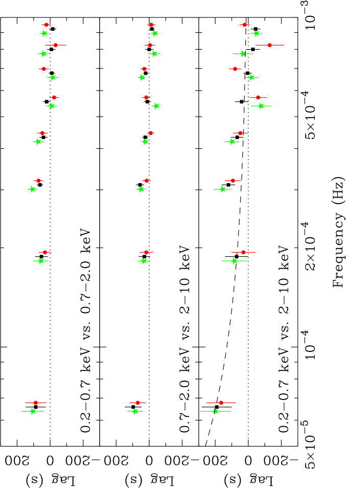
Figure 21: Time lags between light curves in the three energy bands. The symbols are as in Fig. 17. A positive lag indicates the first band leads the second. The dotted line shows the function $\tau(f)=0.013f^{-1}$ discussed in the text.

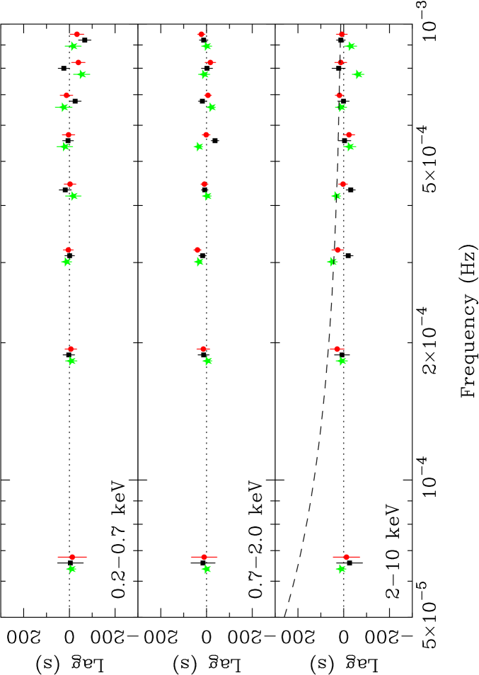
Figure 22: Time lags between light curves from different detectors in the same energy bands. Squares mark pn vs. MOS1, circles mark pn vs. MOS2 and stars mark MOS1 vs. MOS2. As the light curves being compared cover identical energy ranges they should differ only as a result of Poisson noise as so result in zero lag, any lags observed will be a result of Poisson noise. The dotted line shows the function plotted in Fig. 21. As can be seen, the observed lags between bands (Fig. 21) are much larger than those resulting from Poisson noise.

5.3.4 Simulations

The simulated data used in Section 5.2.4 to assess the accuracy of the coherence function were also used to assess the accuracy of the time delay spectrum.

In the first set of simulations the data in the two bands were generated using the same PSD and the same random number sequence. In addition to having unity coherence, the pairs of simulated data also have identical Fourier phases and therefore zero intrinsic phase lag between them. The top panel of Fig. 23 shows the average of the time delay estimates, their standard deviation and the average error estimate from the 100 pairs of simulated data (including Poisson noise as described in Section 5.2.4). This average spectrum is close to the zero-delay expectation meaning that the Poisson noise did not bias the time delay measurements, and the average estimated error is close to the standard deviation of the estimates.

Figure 23: Average time delay measured from simulated data (with zero intrinsic delay). The top panel shows results using light curves with identical PSDs, the bottom panel shows results when different PSDs are assumed for the two light curves. The error bars on the data points represent the standard deviation of the time delay estimates and the lines without data points represent the average of the estimated error bars. The phase is close to zero and the error estimates are close to the expected scatter.

In the second set of simulations the pairs of simulated data were generated using different PSDs for the two bands. The bottom panel of Fig. 23 shows the average time delay spectrum, which again is as expected if the delay estimate is unbiased. It therefore seems reasonable to assume that the time delays observed in MCG–6-30-15 at low frequencies are intrinsic to the source.

6 Discussion

6.1 Summary of results

This paper presents an analysis of the X-ray continuum variability of MCG–6-30-15. A strong, linear correlation is found between the rms variability amplitude and the source flux (Section 3.2). The PSD was examined by fitting model power spectra to the data after allowing for the distorting effects of sampling using a Monte Carlo procedure (Section 4). However, the excellent sampling of the XMM-Newton light curves means that these biases are in any case minimised and so there was a minimum of information lost from the PSD. The PSD is well represented by a power-law of slope $\alpha_{\rm low}=1$ at low frequencies, breaking to a slope of $\alpha\approx 2.5$ at a frequency $f_{\rm br}\approx 10^{-4}$ Hz. However, it should be re-iterated that these PSD results are model-dependent, and that parameterising the PSD using a different model yields slightly different results.

The PSD is energy dependent, with the variations in the higher energy band showing a flatter PSD slope (above the break frequency) than variations in the softer bands. There is no evidence for any energy dependence of the break frequency. Fig. 24 illustrates the PSD shape and energy dependence. Fitting the PSD as a function of energy revealed tentative hints of energy-dependent, high-frequency structure in the PSD (Section 4.4.2). This could be due to subtle instrument effects or may represent low-amplitude structure intrinsic to the source PSD (see also Nandra & Papadakis 2001). These timescales ($\mathrel{\hbox{\hbox to0.0pt{\hbox{\lower 4.0pt\hbox{$\sim$}}\hss}\hbox{$>$}}}10^{-3}$ Hz) are comparable to the dynamical timescale at innermost stable orbit around the black hole. However, further progress on the very high frequency variability of relatively faint sources such as Seyfert galaxies must await future high-throughput missions such as Constellation-X and XEUS.

The variations observed in different energy sub-bands are highly coherent at low frequencies (long timescales) but the coherence falls significantly below unity above $\sim$few $10^{-4}$ Hz, close to the break in the PSD (Section 5.2). The high coherence between soft and hard bands at low frequencies means that the two bands are linked by a single, linear transfer function. The direction and magnitude of the time lag shows that the hard photons lag the soft photons, on average, by $\sim 200$ s at a frequency $f\approx 6\times 10^{-5}$ Hz (Section 5.3). It is not possible to reliably constrain the frequency dependence of the time lags, but the data seem consistent with an approximately $\tau\propto f^{-1}$ dependence of the lag (i.e. constant phase difference $\phi(f)$) similar to that seen in the Seyfert galaxy NGC 7469 (Papadakis et al. 2001) and in GBHCs (Nowak et al. 1999a; Pottschmidt et al. 2000). On shorter timescales the coherence falls well below unity implying there is no simple transfer function relating soft and hard bands.

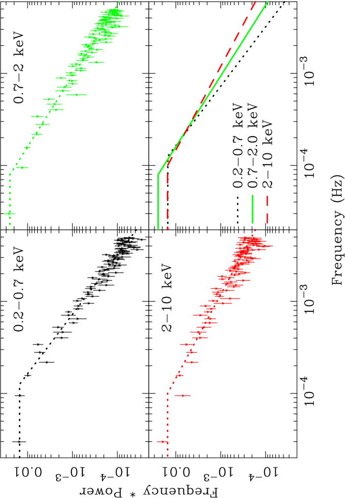
Figure 24: Power spectral data from the three energy bands shown in $fP(f)$ units (dimensionless). The data have be “unfolded” using model 2 to better illustrate the shape of the underlying power spectra. The PSD models are shown with dotted lines, and the error bars show the data/model residuals multiplied by the unfolded PSD model. The bottom right panel shows the three model PSDs overlayed.

6.2 Comparison with previous analyses

Uttley et al. (2002) presented an analysis of long timescale monitoring of MCG–6-30-15 using RXTE. The PSD was found to be best described by a broken power-law with slope of $\alpha_{\rm low}=1$ at low frequencies, breaking to $\alpha=2.0\pm 0.3$ at a frequency $f_{\rm br}=0.13-1.02\times 10^{-4}$ Hz. Using the same PSD model, the break frequency found from the high-frequency XMM-Newton data is $f_{\rm br}=0.6-2.0\times 10^{-4}$ Hz, consistent with the RXTE result. The slope of the PSD above the break is different, but this is most likely an effect of the energy dependence of the PSD. Indeed, using the 2–10 keV XMM-Newton data (i.e. the same energy range used by Uttley et al. 2002) the slope of the high frequency PSD is $\alpha\approx 2.10\pm 0.15$, which is consistent with the RXTE result.

The break frequency presented here (and in Uttley et al. 2002) is model dependent. This is because a model PSD had to be assumed and fitted to the data to derive the appropriate parameters. However, the broken power-law model (with a break to $\alpha_{\rm low}=1$ at low frequencies) provides consistent results when applied to the long timescale RXTE monitoring and the short timescale XMM-Newton observation. This, and the similarity of the observed PSD to those of GBHCs (see Section 6.3) suggests that the chosen model (and therefore the derived break frequency) is reasonable.

Nowak & Chiang (2000) used RXTE and ASCA data to measure the PSD of MCG–6-30-15. They found the PSD to break from $\alpha\approx 0$ to $\alpha\approx 1$ at a frequency $\sim 10^{-5}$ Hz and then break again to $\alpha\approx 2$ in the range $10^{-4}-10^{-3}$ Hz, The position of the high frequency break, as well as the PSD slopes, are roughly consistent with those found from the XMM-Newton data. However, as noted by Uttley et al. (2002), the method employed by Nowak & Chiang (2000) did not account for distorting effects of sampling (see Section 4.1.4) and underestimated the errors at low frequencies. Once these effects are included the low-frequency flattening found by is no longer significant (section 6.2 of Uttley et al. 2002). Nowak & Chiang (2000) also place a limit on any time delay between soft (0.5–2.0 keV) and hard (8–15 keV) bands of $\tau<2000$ s, consistent with the time lag results presented here.

Hayashida et al. (1998) also estimated the PSD of MCG–6-30-15, this time using Ginga data. They found a broken power-law to be a good fit to the data. However, these authors also did not account for the biases in the periodogram, which will be significant due to the patchy sampling of the Ginga light curves. The unusually flat low-frequency slope ($\alpha=-0.5$) found by these authors is most likely a result of bias in the low-frequency periodogram, and therefore the position of their claimed break frequency should be considered with some caution.

The only other AGN for which detailed cross spectral analysis has been performed is NGC 7469 (Nandra & Papadakis 2001; Papadakis et al. 2001). In this object the PSD does not show any significant breaks, but does show the same energy dependence as found in MCG–6-30-15. The present analysis shows that the energy dependence of the PSD is due to the slope of the PSD becoming flatter at higher energies, rather than a change in the break frequency. In addition, NGC 7469 shows time lags between energy bands in the same direction (soft leading hard) and with the similar relative magnitude ($\sim 1$ per cent) as in MCG–6-30-15. Papadakis & Lawrence (1995) showed that in NGC 4051 the harder band showed a flatter PSD than the softer band. Recently, M^cHardy et al. (in prep.) used XMM-Newton data of NGC 4051 and also found this energy dependence of the PDS.

6.3 Comparison with Cygnus X-1

Since EXOSAT first showed the medium timescale PSDs of Seyfert galaxies to have a power-law form, their timing properties have been compared to those of GBHCs. Now, with long timescale monitoring available from RXTE (Edelson & Nandra 1999; Nandra & Papadakis 2001; Uttley et al. 2002) and short timescale observations possible with XMM-Newton (this paper) it is possible to re-assess this comparison.

The best studied GBHC, Cyg X-1, when in its low/hard state shows a PSD with an approximately broken power-law form. The PSD breaks from a low frequency slope of $\alpha\approx 0$ to $\alpha\approx 1$ and then to $\alpha\approx 2$ at high frequencies. The position of the high frequency break is typically $f_{\rm br}\approx 3$ Hz (Belloni & Hasinger 1990; Nowak et al. 1999a). The comparable break in the PSD of MCG–6-30-15 occurs at $f_{\rm br}\approx 10^{-4}$ Hz. This suggests the characteristic timescales in these two systems differ by a factor $\sim 3\times 10^{4}$. Under the assumption that the timescales scale linearly with mass of the central black hole, and assuming Cyg X-1 to contain a $10$ $\rm\thinspace M_{\odot}$ black hole (Herrero et al. 1995), then suggests the mass of the black hole in MCG–6-30-15 is $\sim 3\times 10^{5}$ $\rm\thinspace M_{\odot}$ (in the range 1.5–5.0 $\times 10^{5}$ $\rm\thinspace M_{\odot}$ using the 90 per cent limits on the break frequency in MCG–6-30-15). Assuming a bolometric luminosity of $4\times 10^{43}$ erg s^-1 for MCG–6-30-15 (Reynolds et al. 1997; converting to $H_{0}=75$ km s^-1 Mpc^-1) then implies that MCG–6-30-15 is radiating at the Eddington luminosity. However, since independent mass estimates (such as from reverberation mapping) are not available for MCG–6-30-15 it remains possible that this mass estimate is inaccurate if the relevant timescales do not scale linearly with black hole mass (as assumed above).

If the frequency of the PSD break is related to the orbital frequency of matter close to where the peak emissivity of the accretion disc occurs, $r_{\rm peak}$, then it will depend on $r_{\rm peak}/r_{\rm in}$, where $r_{\rm in}$ is the inner radius of the disc. For a standard disc, $r_{\rm peak}/r_{\rm in}\sim 2$. This will also introduce a dependence on $r_{\rm in}/r_{\rm g}$ (where $r_{\rm g}=GM/c^{2}$ is the gravitational radius of the black hole) and thus the spin parameter of the black hole $a/M$. If the black hole in MCG–6-30-15 has a higher spin parameter than that in Cyg X-1 then the mass deduced from the above scaling could be increased.

The other temporal characteristics seen in MCG–6-30-15 are remarkably similar to those observed in Cyg X-1, implying there is indeed a strong connection between these two types of source. The PSD (above the break frequency) is flatter in harder energy bands in both MCG–6-30-15 and Cyg X-1 (Nowak et al. 1999a; Lin et al. 2000). The strong rms-flux correlation first seen in X-ray binaries (Uttley & M^cHardy 2001) is exhibited by MCG–6-30-15 (see Section 3.2). MCG–6-30-15 also displays a loss of coherence between hard and soft bands at high temporal frequencies (i.e. above the break in the PSD) very similar to that seen in Cyg X-1 (Nowak et al. 1999a) and time lags between these bands that appear similar (in direction and relative magnitude) to those observed in Cyg X-1. In particular, the time lags measured in MCG–6-30-15 between soft and hard bands is $\sim 200$ s in the lowest frequency bin, where the coherence is near unity. In Cyg X-1 the shortest time lags observed are $\sim 2\times 10^{-3}$ s (Nowak et al. 1999a; Pottschmidt et al. 2000) at frequencies just below where the coherence falls significantly below unity. The ratio of these two time lags is $\sim 10^{5}$, similar to the ratio between the PSD break timescales.

It should also be noted that it is not yet clear whether Seyfert galaxies more closely resemble the low/hard or high/soft states of GBHCs (see also the discussion in Uttley et al. 2002). In the high/soft state the PSD of Cyg X-1 is steep at high frequencies ($\alpha\mathrel{\hbox{\hbox to0.0pt{\hbox{\lower 4.0pt\hbox{$\sim$}}\hss}\hbox{$>$}}}2$) and flattens to $\alpha\approx 1$ at $f_{\rm br}\approx 10$ Hz, with no further flattening evident at lower frequencies (Cui et al. 1997; Churazov & Gilfanov & Revnivtsev 2001; Reig, Papadakis & Kylafis 2002). This ratio of characteristic timescales in this case is $\sim 10^{5}$ and the corresponding mass estimate for MCG–6-30-15 is $\sim 10^{6}$ $\rm\thinspace M_{\odot}$, implying a luminosity $\sim 30$ per cent of the Eddington limit. This high (but nevertheless sub-Eddington) accretion rate might be expected if MCG–6-30-15 is indeed in a state similar to the high/soft state seen in Cyg X-1.

It is interesting to note that the best-fitting linear model to the rms-flux correlation observed in MCG–6-30-15 is consistent with passing through the zero-flux origin (Section 3.2). The simplest explanation of this is if there is no significant constant component to the light curve. A strong constant component ($\sim 25$ per cent of the source flux) is observed from the rms-flux correlation in Cyg X-1 (Uttley & M^cHardy 2001), but only when the source is in the low/hard state (Gleissner et al. 2002). This is perhaps also indicating that the variability properties of MCG–6-30-15 are more similar to the high/soft state than the low/hard state of Cyg X-1. (The time delay properties of Cyg X-1 when in its high/soft state are rather similar to those seen in its low/hard state, see e.g. Pottschmidt et al. 2000).

6.4 Physical implications

The X-ray emission mechanism operating in Seyfert galaxies is usually thought to be inverse-Compton scattering of soft photons in a hot corona (e.g. Sunyaev & Titarchuk 1980; Haardt & Maraschi 1991). In the simplest models the harder photons are expected to lag behind the softer photons due to the larger number of scatterings required to produce harder photons, and the delay should be of order the light-crossing time of the corona. The longest observed time delay in MCG–6-30-15 between soft and hard bands is $\sim 200$ s. Assuming a black hole mass of $10^{6}$ $\rm\thinspace M_{\odot}$, this lag corresponds to a light-crossing distance of $\sim 40r_{\rm g}$ ($r_{\rm g}=GM/c^{2}$). Thus the direction and magnitude of the observed lag in MCG–6-30-15 are consistent with an origin in a Comptonising corona. However, if the lags are frequency dependent (as expected by analogy with Cyg X-1 and also seen in NGC 7469; Papadakis et al. 2001) the lags at lower temporal frequencies would become much longer than expected for a compact corona (see discussion in Nowak et al. 1999b). Indeed, the simplest such models predict the time delay between soft and hard photons to be independent of Fourier frequency (Miyamoto et al. 1988), contrary to what is observed. In addition, some models of Compton scattering coronae predict the high frequency PSD should be steeper for higher energy photons, due to the high-frequency fluctuations being washed out by multiple scatterings (Hua & Titarchuk 1996; Nowak & Vaughan 1996), again contrary to the observations.

Alternatively, the time delay between soft and hard bands could be due to the spectral evolution of individual X-ray events. If the spectrum of the event becomes harder as the event unfolds this can lead to an average lag between soft and hard bands. Such models have been discussed by Böttcher & Liang (1998) and Poutanen & Fabian (1999).

Another alternative is that the delay between soft and hard bands could be due to a propagation effect, i.e. a “trigger” signal reaching the soft emission region before the hard emission region. In this scenario the magnitude of the lag is related to the propagation speed and the distance between soft and hard emission regions. The following section describes a model based on this kind of signal propagation.

At higher temporal frequencies the coherence falls well below unity, meaning there is no longer a simple transfer function between the soft and hard band emission. As a static corona should maintain a transfer function (whatever the physical mechanism), on timescales longer than the break in the PSD ($\mathrel{\hbox{\hbox to0.0pt{\hbox{\lower 4.0pt\hbox{$\sim$}}\hss}\hbox{$>$}}}10^{4}$ s), where the coherence is high, the corona may be effectively static (i.e. it maintains its average properties on these timescales). On shorter timescales the corona may be dynamic and so the steep PSD above the break and the loss of coherence may be due to changes in the corona itself.

The timescale of the break in the PSD from $f^{-1}$ to a steeper slope is $10^{4}$ s, which corresponds to a light-crossing distance of $\sim 2\times 10^{4}r_{\rm g}$. The orbital timescale at $40r_{\rm g}$ around a $10^{6}$ $\rm\thinspace M_{\odot}$ black hole is $t_{\rm orb}\sim 10^{3}$ s, while the thermal timescale for a standard, thin accretion disc is $t_{\rm th}\sim 10^{4}$ s (assuming a viscosity parameter $\alpha=0.1$), which is of the same order as the timescale of the break in the PSD. The viscous timescale in such a disc is many orders of magnitude larger than these other timescales (see the discussion of accretion disc timescales in section 5.8 of Frank, King & Raine 1985). However, if that part of the accretion flow responsible for modulating the X-ray emission is geometrically thick, the break in the PSD could correspond to a viscous timescale (which depends on the ratio of disc height $H$ to radius $R$ as $\sim(H/R)^{2}$).

6.5 A phenomenological model

Various models have been considered to explain the variability of GBHCs and Seyfert galaxies. These include: various examples of “shot noise” (e.g. Terrell 1972; Lehto 1989; Merloni & Fabian 2001); rotating “hot spots” on the surface of an accretion disc (Abramowicz et al. 1991; Abramowicz 1992; Bao & Østgaard 1995); occultation by moving clouds (Abrassart & Czerny 2000); self-organised criticality in an accretion disc (Mineshige, Ouchi & Nishimori 1994); fluctuations in the accretion rate propagating through the disc (Lyubarskii 1997; Churazov et al. 2001; Kotov, Churazov & Gilfanov 2001) and magnetohydrodynamic instabilities in the inner accretion disc (Hawley & Krolik 2001).

Most of these models were developed to explain only one aspect of the variations (e.g. its red noise nature). Now, however, it is possible to compare the predictions of these models with the well-determined timing properties of MCG–6-30-15. A viable physical model has to be able to reproduce not only the correct PSD shape and timescales but also the other temporal characteristics such as the rms-flux correlation, the energy dependence of the PSD, the time lags and the coherence. It is not clear whether any of the above mechanism can explain all the observations, and indeed some models (e.g. the obscuration model of Abrassart & Czerny 2000) seem to offer little hope of explaining properties such as the coherence and time lags.

A simple phenomenological model has been developed by Lyubarskii (1997), Churazov et al. (2001), and Kotov et al. (2001) that seems to explain (qualitatively, at least) the temporal properties of Cyg X-1. As the timing properties of MCG–6-30-15 discussed above are very similar to those of Cyg X-1, it is worth discussing this model as a possible explanation for the behaviour of Seyfert galaxies.

In its high/soft state, Cyg X-1 shows a $f^{-1}$ PSD over several decades in frequency (Cui et al. 1997; Churazov et al. 2001; Reig et al. 2002), down to timescales far longer than would normally be associated with the X-ray emitting region itself (which is assumed to be compact). The model put forward by Lyubarskii (1997) to explain this very broad range in timescale has variations in accretion rate occurring over a large range of radii from the central black hole and propagating in towards the X-ray emitting region (assumed to extend over only a few tens of gravitational radii).

If the viscosity parameter of the accretion flow is varying randomly and with the same amplitude at all radii, variations in mass accretion rate at much smaller radii will have an $f^{-1}$ PSD. The accretion rate at the X-ray emitting region (assumed to be concentrated at small radii) is thus being modulated by variations produced over a large range in radius. If the X-ray emission emerging from this region is proportional to the local accretion rate then the X-ray variations will also have an $f^{-1}$ PSD extending down to low frequencies. Each radius produces variations at a characteristic timescale comparable to the timescale for inward propagation, hence long-timescale fluctuations are produced at large radii and shorter-timescale fluctuations are produced closer in. This works because any variations on timescales shorter than the propagation timescale are damped as they move through the disc (see Lyubarskii 1997, and Churazov et al. 2001). This naturally explains both the $f^{-1}$ part of the PSD (i.e. below the high frequency break; Churazov et al. 2001) and the rms-flux correlation (Uttley & M^cHardy 2001).

Once these variations reach the inner regions, where accretion energy is released as X-ray emission, variations on shorter timescales are further suppressed, leading to a steepening of the PSD. Thus the high frequency break in the PSD from $f^{-1}$ to a steeper slope (as seen in MCG–6-30-15) is due to suppression of fluctuations within the X-ray emitting region, and the timescale of the break in the PSD corresponds to the characteristic timescale at the outer radius of the X-ray emitting region (Churazov et al. 2001). The emissivity as a function of radius defines a Green’s function for the incoming $f^{-1}$ fluctuations. In frequency terms, the radial extent of the X-ray producing region makes it act as a “low-pass filter” for the incident $f^{-1}$ fluctuations, resulting in a break in the PSD, to a steeper slope, at high frequencies.

The specific model described by Churazov et al. (2001) has a relatively stable, optically thick, geometrically thin accretion disc sandwiched by an optically thin, geometrically thick corona. The disc produces relatively slowly varying thermal emission (which would emerge presumably in the optical/ultraviolet for a Seyfert galaxy) while it is the variations within the corona that propagate inwards to produce the X-ray variability. The timescale of the high frequency break thus corresponds to the accretion timescale ($\sim$the viscous timescale) of the geometrically thick corona at the outer edge of the X-ray emitting region.

Kotov et al. (2001) extended this model by adding the simple condition that the spectrum of the X-ray emitting region is a function of radius, with the outer regions producing a softer spectrum than the inner regions. This model can then reproduce the observed time lags between soft and hard emission. Accretion rate variations propagating inwards reach the softer emitting region (larger radii) before the harder emitting region (smaller radii), explaining why the soft emission leads the hard. This can explain the energy dependence of the time lags (as delay increases with the separation between energy bands) as well as the frequency dependence (since different radii correspond to different characteristic frequencies as well as different energy spectra). In addition, this model explains the energy dependence of the PSD above the high frequency break. The harder emission is produced from smaller radii, which can be modulated by high frequency fluctuations, hence the harder emission will have more high frequency power than the softer emission (i.e. the hard band PSD will be flatter), as observed (see Fig. 24). Also, as the variations on short timescales are occurring within the X-ray emitting region, i.e. are a result of the dynamic corona, the coherence between bands will fall off at high frequencies, as mentioned in Section 6.4 (see also the discussion in Nandra & Papadakis 2001).

Such phenomenological models require that variations occurring at large radii can be fed into much smaller radii and so influence the PSD. The observed iron line profile of MCG–6-30-15 from this observation (Fabian et al. 2002) indicates that the disc extends down to less than $2r_{\rm g}$, and, from the steep inferred emissivity profile, that much of the X-ray power is generated very close to the black hole. This presents a challenge for all such models, given that the dynamical timescale of this innermost region is $10$–$100$ s, whereas the timescales measured (e.g. the PSD break timescale) are orders of magnitude longer. If the $f^{-1}$ PSD of MCG–6-30-15 is similar to that in the high/soft state of Cyg X-1 (Reig et al. 2002) then the variability timescales will extend to many orders of magnitude longer still. Indeed, the total power in $f^{-1}$ spectra diverges so slowly that the PSD could in principle continue as $f^{-1}$ until very low frequencies without the total power becoming large. (For example, model 2 from Section 4.4 could continue down to the unphysically low frequency $\sim 10^{-28}$ Hz without the integrated power exceeding $F_{\rm var}=1$!)

7 Conclusions

This paper presents a detailed time series analysis of the continuum variability of MCG–6-30-15. The PSD shows a break from $f^{-1}$ to $f^{-2.5}$ at a frequency $f_{\rm br}\sim 10^{-4}$ Hz. Comparing the break timescale with the analogous timescale seen in Cyg X-1, and assuming that these scale linearly with black hole mass, gives a black hole mass of $\sim 10^{6}$ $\rm\thinspace M_{\odot}$ for MCG–6-30-15 and suggests it is accreting at a significant fraction of the Eddington limit. The slope of the PSD above the break is energy dependent, with the harder band showing more high frequency power than the softer band. The variations in different energy bands also become incoherent above the break in the PSD. This leads us to speculate that on timescales shorter than the break timescale, the X-ray emitting corona is dynamic, and that harder photons are produced at smaller radii than softer photons. At the lowest Fourier frequencies the soft and hard bands are highly coherent and the soft band is found to lead the hard band by $\sim 200$ s. The direction and magnitude of this lag is consistent with simple Comptonisation models. A phenomenological model, originally developed to explain the $f^{-1}$ PSD of GBHCs such as Cyg X-1, is discussed and found to be able to reproduce (qualitatively) the observed temporal characteristics of MCG–6-30-15. Although this model is rather simple and phenomenological it can explain the observed temporal characteristics of the X-ray continuum in MCG–6-30-15.

References

- [1] Abramowicz M. A., Bao G., Lanza A., Zhang X.-H., 1991, A&A, 245, 454
- [2] Abramowicz M. A., 1992, in S. Holt, S. G. Neff, C. M. Urry eds. Testing the AGN paradigm, p69
- [3] Abrassart A., Czerny B., 2000, A&A, 356, 475
- [4] Belloni T., Hasinger G., 1990, A&A, 227, L33
- [5] Belloni T., Psaltis D., van der Klis M., 2002, ApJ, 572, 392
- [6] Bendat J. S., Piersol A. G., 1986, Random Data: Analysis and Measurement Procedures, Wiley (New York)
- [7] Bevington P. R., Robinson D. K., 1992, Data Reduction and Error Analysis for the Physical Sciences, McGraw-Hill (New York)
- [8] Bloomfield P., 2000, Fourier Analysis of Time Series, Wiley (New York)
- [9] Bao G., Østgaard E., 1995, ApJ, 443, 54
- [10] Böttcher M., Liang E. P., 1998, ApJ, 506, 281
- [11] Brandt W. N., Boller Th., Fabian A. C., Ruszkowski M., 1999, MNRAS, 303, L58
- [12] Churazov E., Gilfanov M., Revnivtsev M., 2001, A&A, 321, 759
- [13] Cui W., Zhang S. N., Focke W., Swank J. H., ApJ, 484, 383
- [14] Deeter J. E., Boynton P. E., 1982, ApJ, 261, 337
- [15] Done C., Madejski G. M., Mushotzky R. F., Turner T. J., Koyama K., Kunieda H., 1992, ApJ, 400, 138
- [16] Edelson R., Nandra K., 1999, ApJ, 514, 682
- [17] Edelson R., Turner T. J., Pounds K. A., Vaughan S., Markowitz A., Marshall H., Dobbie P., Warwick R. S., 2002, ApJ, 568, 610
- [18] Fabian A. C., 1979, Proc. R. Soc. London, Ser. A, 366, 449
- [19] Fabian A. C. et al. 2002, MNRAS, 335, L1
- [20] Frank J., King A., Raine D., 1985, Accretion Power in Astrophysics, Cambridge Univ. Press (Cambridge)
- [21] Gleissner T., Wilms J., Pottschmidt K., Uttley P., Nowak M. A., Staubert R., 2002, in Ph. Durouchoux, Y. Fuchs and J. Rodriguez eds. Proceedings of the 4th Microquasar Workshop, in press (astro-ph/0207610)
- [22] Green A. R., McHardy I. M., Lehto H. J., 1993, MNRAS, 265, 664
- [23] Green A. R., McHardy I. M., Done C., 1999, MNRAS, 305, 309
- [24] Haardt F., Maraschi L., 1991, ApJ, 380, L51
- [25] Hawley J. F., Krolik J. H., 2001, ApJ, 548, 348
- [26] Herrero A., Kudritzki R. P., Gabler R., Vilchez J. M., Gabler A., 1995, A&A, 297, 556
- [27] Hayashida K., Miyamoto S., Kitamoto S., Negoro H., Inoue H., 1998, ApJ, 500, 642
- [28] Jansen F. et al. 2001, A&A, 365, L1
- [29] Jenkins G. M., Watts, D. G., 1968, Spectral Analysis and its Applications, Holden-Day (San Fancisco)
- [30] Kotov O., Churazov E., Gilfanov M., 2001, MNRAS, 327, 799
- [31] Lampton M., Margon B., Bowyer S., 1976, ApJ, 208, 177
- [32] Lawrence A., Papadakis I., 1993, ApJ, 414, L85
- [33] Leahy D. A., Darbro W., Elsner R. F., Weisskopf M. C., Kahn S., Sutherland P. G., Grindlay J. E., 1983, ApJ, 266, 160
- [34] Lehto H. J., 1989, in J. Hunt, B. Battrick, eds, Two Topics in X Ray Astronomy, (ESA SP-296; Noordwijk: ESA), p499
- [35] Lin D., Smith I. A., Böttcher M., Liang E. P., 2000, ApJ, 531, 963
- [36] Lomb N. R., 1976, Ap&SS, 39, 447
- [37] Lyubarskii Y. E. 1997, MNRAS, 292, 679
- [38] Markowitz A. et al. 2002, ApJ, submitted
- [39] McHardy I. M., 1989, in J. Hunt, B. Battrick, eds, Two Topics in X Ray Astronomy, (ESA SP-296; Noordwijk: ESA), p1111
- [40] Merloni A., Fabian A. C., 2001, MNRAS, 328, 958
- [41] Mineshige S., Ouchi N. B., Nishimori H., 1994, PASJ, 46, 97
- [42] Miyamoto S., Kitamoto S., Mitsua K., Dotani T., 1998, Nature, 336, 450
- [43] Miyamoto S., Kitamoto S., 1989, Nature, 342, 773
- [44] Miyamoto S., Kimura K., Kitamoto S., Dotani T., Ebisawa K., 1991, ApJ, 383, 784
- [45] Mushotzky R. F., Done C., Pounds K. A., 1993, ARA&A, 31, 717
- [46] Nandra K., Papadakis I. E., 2001, ApJ, 554, 710
- [47] Nowak M. A., Vaughan B. A., 1996, MNRAS, 280, 227
- [48] Nowak M. A., Vaughan B. A., Wilms J., Dove J. B., Begelman M. C., 1999a, ApJ, 510, 874
- [49] Nowak M. A., Wilms J., Vaughan B. A., Dove J. B., Begelman M. C., 1999b, ApJ, 515, 726
- [50] Nowak M. A., Chiang J., 2000, ApJ, 531, L13
- [51] Nowak M. A., Wilms J., Dove J. B., 2002, MNRAS, 332, 856
- [52] Papadakis I. E., Lawrence A., 1993, MNRAS, 261, 612
- [53] Papadakis I. E., Lawrence A., 1995, MNRAS, 272, 161
- [54] Papadakis I. E., Nandra K., Kazanas D., 2001, ApJ, 554, L133
- [55] Poutanen J., Fabian A. C., 1999, MNRAS, 306, L31
- [56] Pottschmidt K., Wilms J., Nowak M. A., Heindl W. A., Smith D. M., Staubert R., 2000, A&A, 357, L17
- [57] Press W. H. 1978, Comments on Astrophysics, 7, 103
- [58] Press W. H., Rybicki G. B., 1989, ApJ, 338, 277
- [59] Press W. H., Teukolsky S. A., Vetterling W. T., Flannery B. P., 1992, Numerical Recipes, Cambridge Univ. Press. (Cambridge)
- [60] Priestley M. B., 1981, Spectral Analysis and Time Series, Academic Press (London)
- [61] Rees M. J., 1984, ARA&A, 22, 471
- [62] Reig P., Papadakis I., Kylafis N. D., 2002, A&A, 383, 292
- [63] Reynolds C. S., Ward M. J., Fabian A. C., Celotti A., 1997, MNRAS, 291, 403
- [64] Scargle J. D., 1982, ApJ, 263, 835
- [65] Stella L., Arlandi E., Tagliaferri G., Israel G. L., 1997, in T. Subba Rao, M. B. Priestley, O. Lessi eds., Applications of Time Series Analysis in Astronomy and Meteorology, Chapman & Hall (London) (astro-ph/9411050)
- [66] Strüder L. et al. 2001, A&A, 365, L18
- [67] Sunyaev R. A., Titarchuk L. G., 1980, A&A, 86, 121
- [68] Terrell N. J., 1972, ApJ, 174, L35
- [69] Thorne K. S., 1974, ApJ, 191, 507
- [70] Timmer J., König M., 1995, A&A, 300, 707
- [71] Uttley P., McHardy I. M., 2001, MNRAS, 323, 26
- [72] Uttley P., McHardy I. M., Papadakis I., 2002, MNRAS, 332, 231
- [73] van der Klis M., 1989, in H. Ogelman, E. P. J. van den Heuvel eds., Timing Neutron Stars, Kluwer (Dordrecht), NATO ASI Series C 262, p27
- [74] van der Klis M., 1995, in W. H. G. Lewin, J. van Paradijs, E. P. J. van den Heuvel eds., X-ray Binaries, Cambridge Univ. Press (Cambridge), p252
- [75] van der Klis M., 1997, in G.J. Babu, E. D. Feigelson eds., Statistical Challenges in Modern Astronomy II, Springer-Verlag (New York), p321
- [76] Vaughan B. A., Nowak M. A., 1997, ApJ, 474, L43