QUANTUM EFFECTS AND CLUSTER FORMATION

Abstract

The causal interpretation of quantum mechanics is applied to the universe as a whole and the problem of cluster formation is studied in this framework. It is shown that the quantum effects may be the source of the cluster formation.

I CAUSAL QUANTUM MECHANICS AND GRAVITY

Since the early years of 20th century, there is a causal theory of quantum phenomena called de-Broglie–Bohm theory[1, 2, 3, 4, 5]. It is well proved that the causal theory reproduces all the results of the orthodox quantum theory[4, 5], as well as predicting some new results (such as time of tunneling through a barrier[6]) which in principle lets the experiment to choose between the orthodox and the causal quantum theories. Perhaps the most important point about the causal theory is that it presents a causal deterministic description of the reality. But an important by product of this theory is that enables one to put a step towards constructing a successful quantum gravity theory[7, 8, 9, 10, 11, 12].

The causal quantum theory is based on two postulates[3, 4, 5]:

  First Law:

The physical reality is described by $\{\vec{r}(t);\Psi(\vec{x},t)\}$ where $\vec{r}(t)$ is the position vector of the particle and $\Psi(\vec{x},t)$ is a self–field. Both have a causal evolution. $\Psi(\vec{x},t)$ satisfies an appropriate wave equation (like the Schrödinger equation for a non-relativistic particle) while $\vec{r}(t)$ satisfies Newton’s equation of motion in which there is an additional force called quantum force resulted from $\Psi(\vec{x},t)$. This force can be derived from some quantum potential given by ${\cal Q}=-\frac{\hbar^{2}}{2m}\frac{\nabla^{2}|\Psi|}{|\Psi|}$ for a non relativistic particle.

  Second Law:

The statistical features of the theory is such that the ensemble density is given by $\rho=|\Psi|^{2}$.

So the complete description of the physical reality is given by the following two equations for non–relativistic particles:

$$i\hbar\frac{\partial\Psi}{\partial t}=-\frac{\hbar^{2}}{2m}\nabla^{2}\Psi+V\Psi$$ (1)

$$m\frac{d^{2}\vec{r}}{dt^{2}}=-\left.\vec{\nabla}\left(V+{\cal Q}\right)\right|_{\vec{x}=\vec{r}(t)};\ \ \ \ \ \ {\cal Q}=-\frac{\hbar^{2}}{2m}\frac{\nabla^{2}|\Psi|}{|\Psi|}$$ (2)

The relativistic extension is easy[4, 5]. If one works in the flat Minkowski space–time one should replace the Schrödinger equation with some relativistic wave equation (such as the Klein–Gordon equation for spin zero particles). The quantum potential would be generalized to:

$${\cal M}^{2}=m^{2}(1+{\cal Q})=m^{2}+\alpha\frac{\Box|\Psi|}{|\Psi|};\ \ \ \ \alpha=\frac{\hbar^{2}}{m^{2}c^{2}}$$ (3)

and the equation of motion is given by:

$${\cal M}\frac{dx^{\mu}}{d\tau^{2}}=\left(\eta^{\mu\nu}-\frac{dx^{\mu}}{d\tau}\frac{dx^{\nu}}{d\tau}\right)\partial_{\nu}{\cal M}$$ (4)

It is important to note that ${\cal M}$ plays the role of the (quantum) mass field of the particle[5, 7, 8, 9, 11, 12].

The extension to the curved space–time is trivial[5, 7, 8, 9, 11, 12]:

$${\cal M}^{2}=m^{2}+\alpha\frac{\Box|\Psi|}{|\Psi|};\ \ \ \ \alpha=\frac{\hbar^{2}}{m^{2}c^{2}}$$ (5)

$${\cal M}\frac{dx^{\mu}}{d\tau^{2}}=\left(g^{\mu\nu}-\frac{dx^{\mu}}{d\tau}\frac{dx^{\nu}}{d\tau}\right)\nabla_{\nu}{\cal M}$$ (6)

An important result of all these things is that the quantum effects of matter are in fact geometrical in nature[7]. One can easily transforms the above equation of motion to the ordinary geodesic equation via a conformal transformation of the form[7, 8, 9, 11]:

$$g_{\mu\nu}\rightarrow\widetilde{g}_{\mu\nu}=\frac{{\cal M}^{2}}{m^{2}}g_{\mu\nu}$$ (7)

So that the matter quantum effects are included in the conformal degree of freedom of the space–time metric[7, 11]. A corollary of this result is that one can always work in a gauge (classic gauge) in which no quantum effect be present or in a gauge (quantum gauge) in which the conformal degree of freedom of the space–time metric is identified with the quantum effects of matter[11].

An important question is that if this quantum gravity theory leads to some new results. This theory is investigated for the BigBang and black holes in reference [7, 11]. But here we are interested in investigating whether this theory has anything to do with the cluster formation or clustering of the initial uniform distribution of matter in the universe. The problem of cluster formation is an important problem of cosmology and there are several ways to tackle with it[13]. Here we don’t want to discuss those theories, and our claim is not that the present work is a good one. Here we only state that the cluster formation can also be understood in this way. It is a further task to decide if this work is in complete agreement with experiment or not.

II CLUSTER FORMATION AND THE QUANTUM EFFECTS

In order to investigate if the cluster formation can be viewed as a quantum effect produced by the quantum potential, we consider the universe as a fluid. The hydrodynamics equation is given by:

$${\cal M}\left(\frac{\partial p}{\partial x^{\nu}}g^{\mu\nu}+\frac{1}{\sqrt{-g}}\left(\sqrt{-g}(p+\rho)U^{\mu}U^{\nu}\right)+\Gamma^{\mu}_{\nu\lambda}(p+\rho)U^{\mu}U^{\nu}\right)=\rho\left(g^{\mu\nu}-U^{\mu}U^{\nu}\right)\frac{\partial{\cal M}}{\partial x^{\nu}}$$ (8)

where we have introduced the quantum force in the right hand side just as it is introduced in the equation of motion of a single particle (see equation (6)). It must be noted that the metric itself must be calculated from the corrected Einstein’s equations including the back–reaction terms[7, 11]. In fact one must solve the above equation and the metric equation simultaneously to obtain the metric and the density. We shall not do in this way because solving those equations (equations of references [7, 11]) is difficult. We shall do in a similar way. It is an iterative way and is based on the fundamental assumption of this theory, that is equation (7). As the first order of iteration, we consider the space–time metric as given by the classical Einstein’s equations (Robertson–Walker metric) and solve the above equation for the density, then using the result obtained, calculate the quantum metric using equation (7). Then the new metric can be used to obtain the density at the second order and so on.

In the comoving frame and with the assumption that the universe is in the dust mode ($p=0$) with the flat Robertson–Walker metric, we have from the equation (8):

$$\frac{d\rho^{(1)}}{dt}+3H\rho^{(1)}=0$$ (9)

$$\frac{\partial{\cal Q}^{(1)}}{\partial x^{i}}=0$$ (10)

where ⁽¹⁾ denotes the first order of iteration and $H=\dot{a}/a$ is the Hubble’s parameter. The solution of the above two equations is:

$$\rho^{(1)}=\frac{{\cal X}^{(1)2}}{t^{2}};\ \ \ \ \ \ \ \ \ \ {\cal Q}^{(1)}=\text{constant}$$ (11)

where ${\cal X}^{(1)}$ should yet be determined. The constancy of the quantum potential leads to:

$${\cal Q}^{(1)}=\frac{\alpha}{2}\frac{\Box\sqrt{\rho^{(1)}}}{\sqrt{\rho^{(1)}}}=-\frac{\alpha}{2a^{2}}\frac{\nabla^{2}{\cal X}^{(1)}}{{\cal X}^{(1)}}$$ (12)

so that:

$$\nabla^{2}{\cal X}^{(1)}+\beta{\cal X}^{(1)}=0$$ (13)

where:

$$\beta=\frac{2{\cal Q}^{(1)}a^{2}}{\alpha}$$ (14)

This equation for ${\cal X}^{(1)}$ can simply be solved either in the Cartesian coordinates or in the spherical ones. The solution is:

$${\cal X}^{(1)}=\sin\left(\sqrt{\frac{\beta}{3}}x\right)\sin\left(\sqrt{\frac{\beta}{3}}y\right)\sin\left(\sqrt{\frac{\beta}{3}}z\right)$$ (15)

or:

$${\cal X}^{(1)}=\sum_{l,m}\left(a_{lm}j_{l}(\sqrt{\beta}r)+b_{lm}n_{l}(\sqrt{\beta}r)\right)Y_{lm}(\theta,\phi)$$ (16)

This is the first order approximation. At the second order, one must use the equation (7) to change the scale factor $a^{2}$ to $a^{2}(1+{\cal Q})$, and then from the relation (9) we have:

$$a^{2}(1+{\cal Q})=t^{2/3}{\cal X}^{(1)-4/3}$$ (17)

So that:

$${\cal Q}^{(2)}=-1+{\cal X}^{(1)-4/3}$$ (18)

and then using this form of the quantum potential in the relation (13) or (15) leads to the following approximation for the density:

$$\rho^{(2)}=\frac{1}{t^{2}}\sin^{2}\left(\sqrt{\frac{\gamma}{3}}x\right)\sin^{2}\left(\sqrt{\frac{\gamma}{3}}y\right)\sin^{2}\left(\sqrt{\frac{\gamma}{3}}z\right)$$ (19)

where:

$$\gamma=\frac{2a^{2}}{\alpha}\left(-1+{\cal X}^{(1)-4/3}\right)$$ (20)

and ${\cal X}^{(1)}$ is given by the relation (15). This procedure can be done order by order.

III RESULTS

In the figures (1), (2), (3), (4) and (5) the density at four times are shown and the clustering can be seen easily. These figures are plotted using the solution in the Cartesian coordinates.

In figures (6), (7), (8), (9) and (10) the $(l,m)=(00)$ mode of equation (16) is shown at five time steps.

In figures (11), (12), (13), (14) and (15) the $(11)\oplus(1-1)$ mode is shown at five time steps.

The second order solution (19) is shown in figure 16, where both large scale and small scale structures are shown.

It is important to note that the clustering can be seen in any of these figures. In the last figure, however, one observes that at the large scale the universe is homogeneous and isotropic, while at the small scale these symmetries are broken.

At the end, in order to see whether or results are in agreement with the observed clustering, the correlation function ($\xi(r)$) is obtained from the third order of iteration and is compared with the cases $\xi=(r/r_{0})^{-\gamma}$ with $\gamma=1.8$ and $\gamma=3$ and with the standard result of a typical $P^{3}M$ code[13]. As it can be seen in figure (17) our results are in good agreement with the $P^{3}M$ code and with observation.

As we stated previously, our claim here is not that this theory is a good one for the cluster formation problem. But it is only claimed that in the framework of causal quantum theory, the quantum force may be a cause for the cluster formation.

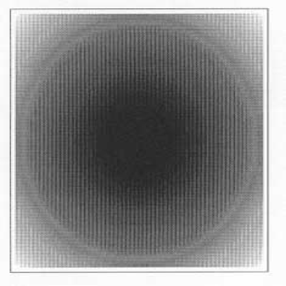
FIG. 1.: Cartesian mode after expansion by the factor 1.1

$\rightarrow$

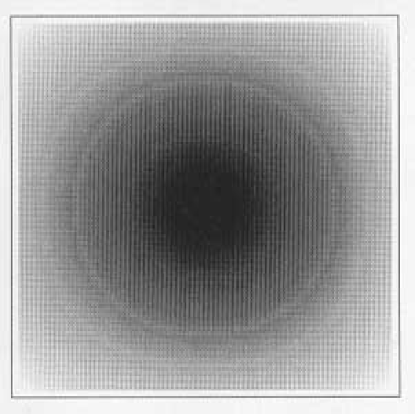
FIG. 2.: Cartesian mode after expansion by the factor 1.2

$\rightarrow$

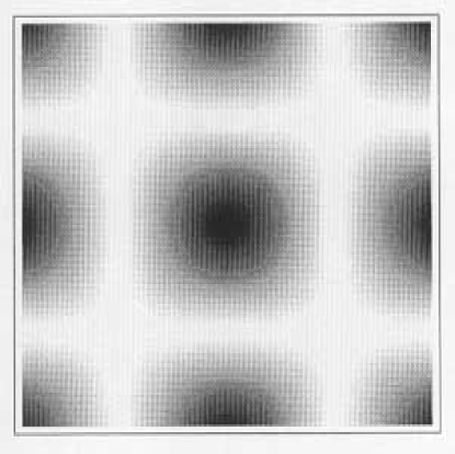
FIG. 3.: Cartesian mode after expansion by the factor 3

$\rightarrow$

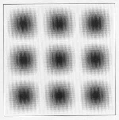
FIG. 4.: Cartesian mode after expansion by the factor 5

$\rightarrow$

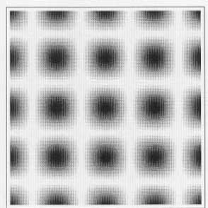
FIG. 5.: Cartesian mode after expansion by the factor 6

$\rightarrow$

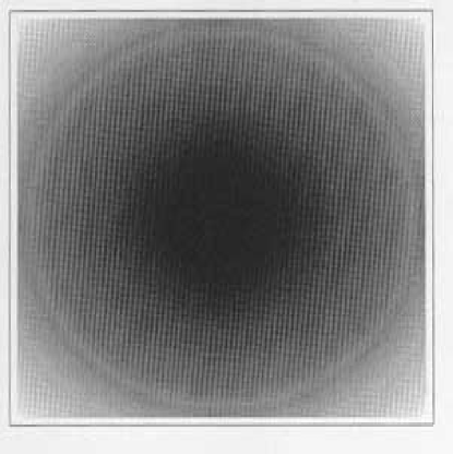
FIG. 6.: $(00)$ mode after expansion by the factor 1.1

$\rightarrow$

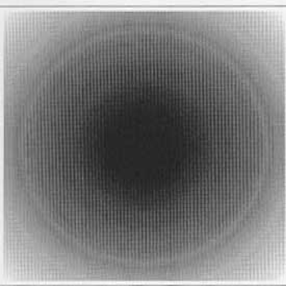
FIG. 7.: $(00)$ mode after expansion by the factor 1.2

$\rightarrow$

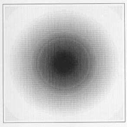
FIG. 8.: $(00)$ mode after expansion by the factor 3

$\rightarrow$

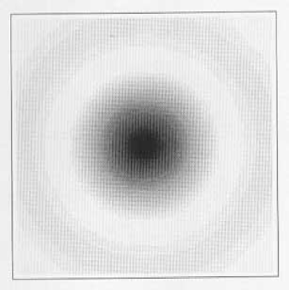
FIG. 9.: $(00)$ mode after expansion by the factor 5

$\rightarrow$

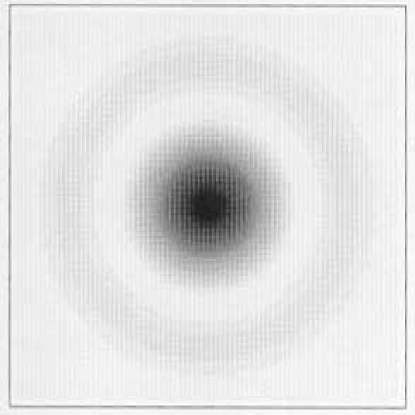
FIG. 10.: $(00)$ mode after expansion by the factor 6

$\rightarrow$

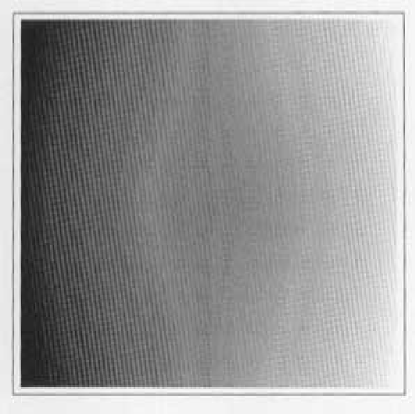
FIG. 11.: $(11)\oplus(1-1)$ mode after expansion by the factor 1.2

$\rightarrow$

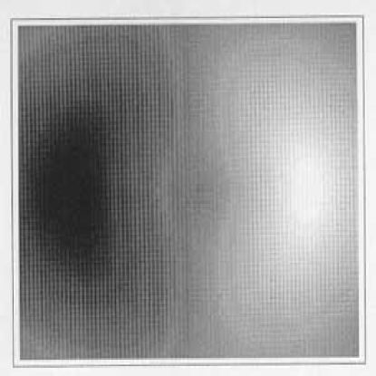
FIG. 12.: $(11)\oplus(1-1)$ mode after expansion by the factor 3

$\rightarrow$

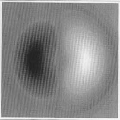
FIG. 13.: $(11)\oplus(1-1)$ mode after expansion by the factor 5

$\rightarrow$

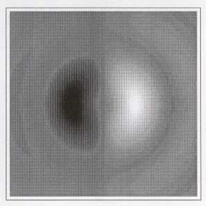
FIG. 14.: $(11)\oplus(1-1)$ mode after expansion by the factor 6

$\rightarrow$

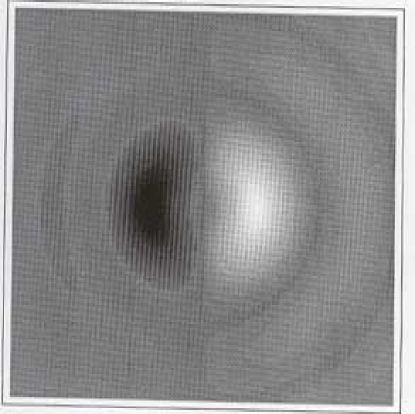
FIG. 15.: $(11)\oplus(1-1)$ mode after expansion by the factor 8

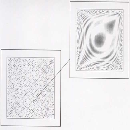
FIG. 16.: Second order solution after expansion by the factor 8

$\rightarrow$

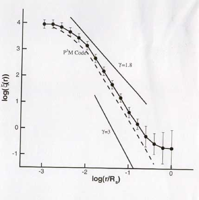
FIG. 17.: Correlation function after expansion by the factor 8

REFERENCES

- [1] L. de-Broglie, Journ. de Phys., 5, 225, (1927).
- [2] L. de-Broglie, Annales de la Fondation Louis de Broglie, Vol. 12, No. 4, (1987).
- [3] D. Bohm, Phys. Rev. 85, 166 (1952); D. Bohm, Phys. Rev. 85, 180 (1952).
- [4] D. Bohm and J. Hiley, The Undivided Universe (Routledge, 1993).
- [5] P.R. Holland, The Quantum Theory of Motion (Cambride University Press, 1993).
- [6] Bohmian Mechanics and Quantum Theory: An Appraisal (Boston Studies in the philosophy of science, Vol. 184), Ed. J.T. Cushing, A. Fine, and S. Goldstein, (Kluwer Academic Publishers, 1996).
- [7] F. Shojai and M. Golshani, Int. J. Mod. Phys. A, Vol. 13, No. 4, 677, (1998).
- [8] F. Shojai, A. Shojai and M. Golshani, Mod. Phys. Lett. A, Vol. 13, No. 34, 2725, (1998).
- [9] F. Shojai, A. Shojai and M. Golshani, Mod. Phys. Lett. A, Vol. 13, No. 36, 2915, (1998).
- [10] A. Shojai, F. Shojai and M. Golshani, Mod. Phys. Lett. A, Vol. 13, No. 37, 2965, (1998).
- [11] A. Shojai, Int. J. Mod. Phys. A, Vol. 15, No. 12, 1757, (2000).
- [12] F. Shojai and A. Shojai, Int. J. Mod. Phys. A, Vol. 15, No. 13, 1859, (2000).
- [13] See for example: G. Börner, The Early Universe, third edition, (Springer-Verlag, Berlin Heidelberg 1993), and references therin.