Synchrotron Radiation at Radio Frequencies

from Cosmic Ray Air Showers 

Denis A. Suprun$\,{}^{a}$ , Peter W. Gorham$\,{}^{b}$  and Jonathan L. Rosner$\,{}^{a}$ 

^a Enrico Fermi Institute and Department of Physics

University of Chicago, 5640 S. Ellis Avenue, Chicago, IL 60637

^b Department of Physics and Astronomy, University of Hawaii at Manoa

2505 Correa Rd., Honolulu, HI 96822

ABSTRACT

We review some of the properties of extensive cosmic ray air showers and describe a simple model of the radio-frequency radiation generated by shower electrons and positrons as they bend in the Earth’s magnetic field. We perform simulations by calculating the trajectory and radiation of a few thousand charged shower particles. The results are then transformed to predict the strength and polarization of the electromagnetic radiation emitted by the whole shower.

PACS numbers: 96.40.Pq; 95.30.Gv; 41.60.Ap; 41.60.-m

I Introduction

In the next few years the giant Pierre Auger air shower array will start operating in the Southern Hemisphere, to be followed by a Northern Hemisphere companion. The area covered by these arrays will be large enough to allow detection of showers with energies higher than $10^{20}$ eV. The radiation properties of such energetic showers differ from those with energies up to $10^{17}$ eV that were routinely studied by smaller arrays. Particular attention should be paid to the fact that very energetic air showers develop to their maximum not far from the Earth’s surface. While the typical altitude of the maximum of a $10^{17}$ eV shower is located at 625 g/cm² [1], i.e. at 4 km elevation, a $10^{20}$ eV shower maximum approaches $1$ km above sea level. This is about the same elevation as that of many ground detectors. The maxima of the most energetic showers will not be observed overhead but rather from the side. The differences in the position and the distance to the shower maxima affect the intensity and polarization of the radiation emitted by these showers.

Many studies are concentrated on understanding the coherent Cherenkov radio emission from the excess charge in high energy showers developing in dense media [2, 3, 4, 5]. In air showers, however, another radiation mechanism dominates the Cherenkov radiation. It is associated with the acceleration that charged particles of the shower experience in the Earth’s magnetic field [6, 7]. This mechanism would occur even if there were no excess charge in air showers. Electrons and positrons bend in the opposite directions in a magnetic field. However, the opposite signs of their accelerations are cancelled by the opposite signs of the electric charges. As a result, the electromagnetic radiation from both particles of an electron-positron pair is coherent, becoming the main source of the air shower radio emission [8]. In this paper we develop a simple radiation model which can be applied to most geometries relevant to extensive air showers.

In Section II we consider the electric field produced by a single accelerated charged particle. Previous experimental studies of the shower radiation strength are discussed in Section III. Section IV reviews shower pancake structure and restrictions it imposes on the choice of the radiation model. Coherence of shower particle radiation is considered in Section V, while Sections VI and VII give details and results of the Monte Carlo simulations. We summarize in Section VIII. Details of the radiation calculations and symmetries of the radiation patterns are given in an Appendix.

II Radiation from accelerated charges

Numerous experiments have confirmed acceleration of charged particles in the Earth’s magnetic field as the main source of the electromagnetic radiation from an extensive air shower (see in particular [9] and several other articles in [10]). For a $10^{17}$ eV shower with a maximum high above the Earth the radiation of each gyrating particle can be understood as familiar synchrotron radiation [11]. Even in this case the significant lateral and longitudinal spread of the shower particles hinders simple analytical calculation of the total electromagnetic radiation. For a $10^{20}$ eV shower the distance between the maximum and an antenna detecting the radio-frequency radiation could be comparable to the radiation length of an electron (36.7 g/cm², or 330 m at an altitude of $1$ km). This means that the displacement of a radiating particle is significant and the direction from it towards the antenna appreciably changes during the motion. As a result, the usual synchrotron formulae are not easily applicable even for a single electron. Instead, we start from the underlying formula for a radiating particle [12, 13]:

$${\bf E}({\bf x},t_{a})=\frac{e\mu}{4\pi\epsilon_{0}}\,\left[\frac{{\bf n}-n\boldsymbol{\beta}}{\gamma^{2}|1-n\boldsymbol{\beta}\cdot{\bf n}|^{3}\,l^{2}}\right]_{\rm ret}+\frac{e\mu}{4\pi\epsilon_{0}c}\,\left[\frac{{\bf n}\times\left[({\bf n}-n\boldsymbol{\beta})\times\dot{\boldsymbol{\beta}}\right]}{|1-n\boldsymbol{\beta}\cdot{\bf n}|^{3}\,l}\right]_{\rm ret}$$ (1)

which is correct regardless of the distance to the antenna. In this formula $\boldsymbol{\beta}$ is the velocity vector in units of $c$, $\dot{\boldsymbol{\beta}}=d\boldsymbol{\beta}/dt$ is the acceleration vector, divided by $c$, ${\bf n}$ is a unit vector from the radiating particle to the antenna, and $l$ is the distance to the particle. $\mu\approx 1$ denotes the relative magnetic permeability of air, $n$ the index of refraction. The square brackets with subscript “ret” indicate that the quantities in the brackets are evaluated at the retarded time, not at the time $t_{a}$ when the signal arrives at the antenna.

The first term decreases with distance as $1/l^{2}$ and represents a boosted Coulomb field. It does not produce any radiation. The magnitudes of the two terms in Eq. (1) are related as $1/(\gamma^{2}l)$ and $|\dot{\boldsymbol{\beta}}|/c$. The characteristic acceleration of a 30 MeV electron ($\gamma\approx 60$) of an air shower in the Earth’s magnetic field ($B\approx 0.5$ Gauss) is $|{\bf a}|=ecB/(\gamma m)\approx 4.4\cdot 10^{13}$ m/s². Even when an electron is as close to the antenna as 100 m, the first term is two orders of magnitude smaller than the second and can be neglected. The second term falls as $1/l$ and is associated with a radiation field. It describes the electric field of a single radiating particle for most geometries relevant to extensive air showers. It can be shown [14] to be proportional to the apparent angular acceleration of the charge up to some non-radiative terms that are proportional to $1/l^{2}$. This relation is referred to in the literature as “Feynman’s formula.” Sometimes it is used for the purposes of Monte Carlo simulation [15]. For us, however, the explicit expression for the electric field in terms of velocity and acceleration in Eq. (1) turns out to be more convenient.

III Experimental observations

The collaboration of H. R. Allan at Haverah Park in England [8] studied the dependence of radiation strength on primary energy $E_{p}$, perpendicular distance $R$ of closest approach of the shower core, zenith angle $\theta$, and angle $\alpha$ between the shower axis and the magnetic field vector. Their results indicate that the electric field strength per unit of frequency, ${\cal E}_{\nu}$, could be expressed as

$${\cal E}_{\nu}=s_{r}\,\frac{E_{p}}{10^{17}\,{\rm~{}eV}}\,\sin\alpha\,\cos\theta\,\exp\left(-\frac{R}{R_{0}(\nu,\theta)}\right)~{}~{}~{}\mu{\rm V}/{\rm m}/{\rm MHz}~{}~{}~{},$$ (2)

where $R_{0}$ is an increasing function of $\theta$, equal (for example) to $(110\pm 10)$ m for $\nu=55$ MHz and $\theta<35^{\circ}$. The equation is valid for $E_{p}$ between $10^{17}$ and $10^{18}$ eV and for $R$ less than 300 m. Originally, the value of the calibration factor was determined to be $s_{r}=20$. It was subsequently updated in [16] to yield field strengths approximately 12 times weaker, corresponding to $s_{r}=1.6$, while observations in the U.S.S.R. gave field strengths approximately 2.2 times weaker ($s_{r}=9.2$). The latter two values of $s_{r}$ were obtained with approximately 10 times higher statistics and are a better indication of the shower radiation strength. Still, some question persists about the magnitude of the effect, serving as an impetus to further measurements.

We will describe a simple model of air shower radiation and then test if it gives radiation strength corresponding to values of $s_{r}$ in the range from 1 to 10. We will take into account some characteristics of the Haverah Park site, namely, its elevation (220 m), the Earth’s magnetic field strength ($B=0.49$ Gauss) and inclination ($\gamma_{d}=68^{\circ}$).

IV Radiation model and pancake structure

We begin by making a simplifying assumption that radiation only comes from the shower maximum and lasts as long as particles travel through one radiation length ($\sim$1 $\mu$s). The total number $N_{e}$ of charged particles at the shower maximum is approximately 2/3 per GeV of primary energy [17]. We will also assume equal numbers of 30 MeV positrons and electrons among charged particles, neglecting an admixture of muons, an excess of electrons and variations of energies between the particles. Such a simple model serves as a precursor to a future full scale shower development and radiation simulation similar to a study of the properties of electromagnetic showers in dense media performed in [13]. Now we review lateral and longitudinal particle distributions in the shower pancake.

Lateral particle density $\rho_{e}$ is parameterized by the age parameter $s$ of the shower ($s=1$ for the shower maximum) and the Molière radius $r_{m}$ [18, 19, 20]:

$$\rho_{e}=K_{N}\,\left(\frac{r}{s_{m}r_{m}}\right)^{s-2}\,\left(1+\frac{r}{s_{m}r_{m}}\right)^{s-4.5},$$ (3)

where

$$K_{N}=\frac{N}{2\pi s_{m}^{2}r_{m}^{2}}\,\frac{\Gamma(4.5-s)}{\Gamma(s)\Gamma(4.5-2s)},$$ (4)

$\Gamma$ is the gamma function, $r$ the distance from the shower axis, $N$ the total number of charged particles, and $s_{m}=0.78-0.21s$. The Molière radius for air is approximately given by $r_{m}=74\,(\rho_{0}/\rho)$ m, with $\rho_{0}$ and $\rho$ being the air densities at sea level and the altitude under consideration, respectively.

As a shower travels towards the Earth and enters denser layers of the atmosphere, the age parameter increases while the Molière radius drops. Both processes affect the spread of the lateral distribution. The influence of the age parameter appears to be more significant. As it grows, the average distance of the shower particles from its axis increases. This effect overcomes the influence of a smaller Molière radius which tends to make the lateral distribution more concentrated towards the axis. For a fixed age parameter $s$, however, the Molière radius is the only quantity that determines the spread of the lateral distribution. At shower maximum ($s=1$) the average distance from the axis can be calculated to be $(2/3)s_{m}r_{m}=0.38\,r_{m}$.

The thickness of the shower pancake was also taken into account. It is directly related to the average dispersion in arrival times of air shower particles. At a distance $r$ from the axis it is described in [21] by:

$$\sigma_{t}=\sigma_{t_{0}}\,\left(1+\frac{r}{r_{t}}\right)^{b},$$ (5)

where $\sigma_{t_{0}}=1.6$ ns, $r_{t}=30$ m and $b=(2.08\pm 0.08)-(0.40\pm 0.06)\sec\theta+(0\pm 0.06)\log(E_{p}/10^{17}~{}{\rm eV})$, for $r<2$ km, $10^{17}<E_{p}<10^{20}$ eV and $\theta<60^{\circ}$. This empirical formula reflects an increase of the pancake thickness at greater distances from the shower axis. It was derived from measurements performed at an altitude of 1800 m in New Mexico. For vertical showers it gives $b=1.68$.

For those showers that reach their maximum at 1800 m above sea level, one can use the lateral distribution (3) to calculate the average $\sigma$ of the shower pancake thickness at this altitude: $\sigma_{0}=8.4$ ns. For simplicity, we will assume that the longitudinal distribution is independent of distance from the axis and has a constant dispersion $\sigma_{0}$.

The shape of the longitudinal distribution is defined by multiple scattering of electrons in the atmosphere. One can expect a sharp increase of particle number at the bottom of the pancake where virtually unscattered high energy particles are concentrated, followed by a slow decay at the top of the pancake as slower electrons increasingly lag behind. This presumption was confirmed in [22] with the shape function being measured to be proportional to $t^{2}\exp(-t/\tau)$.

Unfortunately, the thickness of the pancake was not measured at various altitudes above sea level. We would like to know the longitudinal distribution at shower maximum, but the pancake thickness is known only at 1800 m. To circumvent this problem, we choose a shower of such energy that it develops to its maximum at about 1800 m altitude. Locations of the maxima of $10^{17}$ to $10^{18.3}$ eV showers were measured by the HiRes/MIA hybrid detector to lie higher in the atmosphere [1]. They also obtained evidence of change from a heavy to a light composition in this energy region. If the elongation rate remains constant for even higher energies that would indicate that the primaries become exclusively protons at about $10^{19}$ eV. Simulations using the SIBYLL high energy hadronic interaction model show [1, 23] that $10^{19}$ eV protons produce showers with maxima at 820 g/cm². This corresponds to 1800 m altitude above sea level for vertical showers. For these showers Eq. (5) gives a longitudinal distribution of charged particles exactly at shower maximum. Only for these showers do we know both lateral and longitudinal distributions at their maxima.

Thus, in the model we will use a vertical $10^{19}$ eV shower which develops to its maximum of approximately $0.33\cdot 10^{10}$ electrons and $0.33\cdot 10^{10}$ positrons at 1800 m above sea level. The lateral distribution of the pancake is described by Eq. (3) while the longitudinal distribution follows a $t^{2}\exp(-t/\tau)$ shape. The time constant $\tau$ was chosen to be equal to $\sigma_{0}/\sqrt{3}$. This ensures that the dispersion of the longitudinal distribution is $\sigma_{0}=8.4$ ns, or $2.5$ m. The pancake profile described in this Section is shown in Fig. 1.

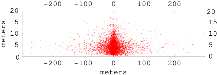
Figure 1: Top and side view of a shower pancake of a vertical $10^{19}$ eV shower at its maximum. The distributions of 10000 pancake particles are shown. The average radial spread is 33 m. The average delay of pancake particles is 4.4 m behind the central pair at the bottom of the pancake.

V Coherence of pancake radiation

The question remains if Eq. (2) correctly describes the radiation from a $10^{19}$ eV shower. One does expect a linear growth of the pulse amplitude as the number of radiating particles increases with shower energy. The coherence of the emitting particles is an underlying assumption. It is valid for radiation at RF wavelengths of several meters coming from the main bulk of the particle swarm concentrated around the shower axis. This simple argument is modified by two competing effects.

A greater penetration of the atmosphere by a more energetic shower means that the shower develops to its maximum at a lower altitude with a higher air density. The Molière radius $r_{m}$ is smaller at this altitude and Eq. (3) predicts a more concentrated lateral distribution of the shower particles. As a result, the RF radiation of the shower should become more coherent and stronger. Thus, the pulse amplitude should increase more rapidly than linearly with primary energy.

However, this effect is offset by the fact that charged accelerating particles radiate mostly in the direction of their velocities. For a fixed distance $R$ from antenna to the axis of a vertical shower, the angle $\delta$ between the vectors ${\bf n}$ and $\boldsymbol{\beta}$ becomes larger (see Fig. 2) and the electric field smaller as the altitude decreases. This can be seen directly from Eq. (1). Considering small angles $\delta$ and taking the index of refraction of air $n=1$ for simplicity, one can write its denominator as $(1-\cos\delta)^{3}l\propto\delta^{6}(R/\delta)\propto\delta^{5}$. The magnitude of the numerator can be shown to be proportional to $R^{2}/h^{2}$ [24], i.e., to $\delta^{2}$. As a result, the electric field $E\propto\delta^{-3}$ and decreases at lower altitudes. This should lead to a smaller pulse amplitude than expected from a linear growth with shower energy.

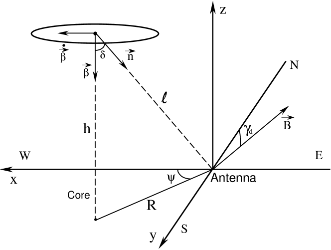
Figure 2: Geometry of a vertical shower. Axes relative to antenna are $x$ (magnetic West), $y$ (magnetic South) and $z$ (up). Vector B lies in the $yOz$ plane. The ellipse shows the plane of a “slice”: an infinitely thin horizontal layer of the shower pancake.

The combination of different factors fortuitously leads to an overall linear dependence of pulse amplitude on primary energy in the range between $10^{17}$ and $10^{18}$ eV, as shown in Eq. (2). As the primary energy approaches $10^{19}$ eV, there is some evidence that the radiation strength increases less rapidly than $E_{p}$ [8]. Thus, we expect that for a $10^{19}$ eV shower the calibrating factor $s_{r}$ in Eq. (2) shifts down to the lower end of the 1 to 10 range.

VI Monte Carlo details

Calculation of the signal from $10^{10}$ particles is impossible with a limited computing time. Instead, we start with a calculation of radiation from an infinitely thin horizontal pancake slice located at 1800 m elevation. $10^{4}$ electron-positron pairs were chosen randomly from this slice according to the expected lateral distribution (see Fig. 1, top panel). The geomagnetic distortion of the axial symmetry of the pancake was not taken into account. The initial velocity of particles was assumed to be vertical. Then, the trajectory, velocity and acceleration in the Earth’s magnetic field of each gyrating particle were calculated according to Eqs. (7-13) (see Appendix). After taking into account the delay associated with the propagation of the electromagnetic wave, we compute the electric field perceived by the ground based antenna located at 220 m above sea level. The East-West electric field components from different pairs are summed up to simulate the electromagnetic pulse detected by the EW-oriented antenna.

Figure 3: The EW component $E_{EW}$ of the electromagnetic pulse of $10^{4}$ radiating electron-positron pairs distributed over a horizontal slice at 1800 m above sea level. The axis of the slice is located 200 m South of the antenna. The time axis was chosen in such a way that the pulse of a pair located at the axis of the slice starts at time 0. The earliest possible arrival time is $-42$ ns and comes from pairs located right above the antenna. Those pairs are too far from the axis (200 m being much larger than the average spread of $0.38\,r_{m}=33$ m) and the statistics for them is not sufficient.

In the process of motion charged particles become closer to the antenna. As a result, the observed pulse duration is much shorter than the real radiation time of the order of 1 $\mu$s. The radiation from different pairs does not arrive at the same time but the short individual pulses overlap to form a “slice” pulse. The statistics is high enough for the particles around the shower axis and the pulse amplitude becomes asymptotically proportional to the number of radiating particles. That allows us to determine the electromagnetic pulse from an arbitrary high number of particles in the slice by simple scaling. The pulses from pairs that are further from the center overlap only slightly. As a result, the net pulse from the distant particles is not smooth and displays statistical jitter. It is not proportional to the number of particles involved. With a limited computing time one cannot avoid this problem. We do not amplify random fluctuations by scaling them to a higher statistics. Instead, we try to determine the region of “sufficient statistics”. To do that we take the ratio of the pulse produced by 10000 pairs and the pulse produced by 5000 pairs. The time interval where this ratio is within 25% from 2 is assumed to be the region of sufficient statistics and eligible for scaling to a higher number of pairs. Fig. 3 shows the shape of the slice pulse $E(t_{a})$ in the region of sufficient statistics. The fraction of particles that produce radiation in this time interval is 96.7%. It is a representative fraction of the total radiation. We will neglect the radiation outside of this time interval.

Figure 4: The EW component $E_{EW}$ of electromagnetic pulse of $0.33\cdot 10^{10}$ radiating electron-positron pairs distributed over the thickness of the shower pancake at 1800 m above sea level. The axis of the pancake is located 200 m South of the antenna. The time axis was chosen in such a way that the pulse produced by a pair located in the axis at the bottom of the pancake starts at time 0.

Figure 5: The Fourier transform of the electromagnetic pulse shown in Fig. 4. The spectrum is very flat below 2 MHz. The limited statistics of the model results in some jitter at 200$-$500 MHz. The spectrum above 500 MHz is not shown because the statistics is not sufficient to make reliable predictions of the Fourier components at these high frequencies.

Now that the slice pulse is determined, we take into account that slices are longitudinally distributed according to the $t^{2}\exp(-t/\tau)$ formula, $\tau=\sigma_{0}/\sqrt{3}$. The dispersion of their distribution $\sigma_{0}=8.4$ ns corresponds to the distance of 2.5 m. It is very small compared to the distance between the shower pancake and the antenna. Therefore, each horizontal slice produces the same signal as the one shown in Fig. 3, only shifted in time. As a result, the problem of calculating the pancake pulse reduces to the integration of appropriately weighted and shifted slice pulses. The result is scaled up for $0.33\cdot 10^{10}$ pairs and shown in Fig. 4. Fig. 5 gives the Fourier transform $E_{\nu}$ of the pancake pulse. The nonzero thickness of the pancake translates into a longer pancake pulse in comparison with the slice pulse, thereby limiting the main part of the radiation spectrum to the frequencies below 100 MHz.

VII Results and discussion

Figure 6: The East-West component of the field strength $|{\cal E}_{\nu EW}|$ at 55 MHz as a function of distance from the shower axis. The dashed line is the best fit of formula (2) to the Monte Carlo results. The calibrating parameter for the fit is $s_{r}=1.27$. The solid line is the best exponential fit with characteristic distance $R_{0}=43.7$ m. The statistical uncertainties from repeated Monte Carlo simulations are smaller than sizes of the dots. Nevertheless, they were taken into account during fitting procedures.

Radio pulse spectrum.

The spectrum (Fig. 5) shows a clear power law falloff between 40–500 MHz, approximately $\sim 1/\nu^{4.5}$. This observation can be compared to the measurements [25] of the radiation spectrum that observed that the field strength $|{\cal E}_{\nu}|$ goes as $1/\nu$ between 1–500 MHz. However, these measurements were admittedly inconclusive [8] because they effectively averaged the spectral distribution over different distances between antenna and shower core. At large distances $R$ from the axis the radio pulse becomes longer. In our model the main part of the signal is concentrated in the first 50 ns for $R=100$ m but increases to about 150 ns for $R=300$ m. This leads to a loss of high frequency components and the spectrum is expected to be steeper at larger core distances. The expectation that the spectrum shape may be different at different distances led to a conclusion that the measured $1/\nu$ spectrum is not of any fundamental significance but simply reflects the characteristics of the detecting array. One can only expect that for a fixed $R$ the spectrum decreases with frequency. There is a general agreement between the predicted spectrum for $R=200$ m (Fig. 5) and this expectation.

It is worth noting that particles of different energies are present in a real shower pancake. Those with lower energies increasingly lag behind. The lower the energy of a particle, the later its radiation arrives to the antenna. This radiation is also stronger for low energy particles experience higher accelerations. As a result, the pulse of the real pancake differs from the one in Fig. 4 in that its peak occurs at a later time and, more importantly, its width is larger. The preponderance of low frequency components in the spectrum of the real pancake should be even more prominent than that of Fig. 5.

Variation of field strength with distance to the antenna.

We calculated electromagnetic pulses for the pancakes whose axes are located at various distances $R$ South of the antenna. To compare with the Haverah Park measurements [8] we show the variation of the East-West component of the field strength $|{\cal E}_{\nu EW}|$ at 55 MHz with distance $R$ (Fig. 6).

A power law fitting these results would rise too fast at distances smaller than 100 m. It makes more sense to use an exponential fit. We can fit formula (2) to the results of the Monte Carlo simulation. For $10^{19}$ eV vertical showers at the Haverah Park site, this formula becomes ${\cal E}_{\nu}=100s_{r}\cos\gamma_{d}\exp(-R/R_{0})=37.5s_{r}\exp(-R/110)$. The best fit is provided by the calibrating factor $s_{r}=1.27$. This value is indeed in the lower end of 1 to 10 range, as expected for the $10^{19}$ eV shower. One can tell that even this simple model is successful in predicting the order of magnitude of the electromagnetic pulse emitted by the extensive air showers.

The best exponential fit, however, is provided not by Eq. (2) with $R_{0}=110$ m, but by an exponential with characteristic decay distance $R_{0}=43.7$ m. This may be a consequence of either the limited nature and simplicity of this model or the great experimental difficulties besetting the detection and calibrating radio pulses from the extensive air showers. A future full scale shower development simulation and a possible equipment of the Auger experiment with RF detecting antennas will clarify this issue.

Variation of field strength with angle $\psi$.

Consider the frame centered at the antenna, with axis $Ox$ going to the magnetic West, $Oy$ to the South and $Oz$ directly up. The initial velocity of all charged particles is assumed to be vertical: $\boldsymbol{\beta}=(0,0,-1)$, while the initial acceleration $\dot{\boldsymbol{\beta}}$ is parallel to $Ox$, or, in other words, to the $(1,0,0)$ vector (see Fig. 2). Electrons bend towards the magnetic West and positrons towards the East. The electric fields from both particles of an electron-positron pair are coherent; the opposite signs of their accelerations are cancelled by the opposite signs of the electric charges.

Let $\psi$ be the angle between $Ox$ and the direction to the shower core, $R$ the distance to the core, and $h$ the altitude of the radiating particle above the antenna. The denominator of the second term of Eq. (1) is independent of $\psi$. The numerator determines that, to leading (second) order in $R/h$, the initial electric field vector ${\bf E}$ received at the antenna lies in the horizontal plane and is parallel to $(\cos 2\psi,\sin 2\psi,0)$ [24]:

$${\bf E}\ \|\ (\cos 2\psi,\sin 2\psi,0)$$ (6)

The magnitude of the numerator is independent of the angle $\psi$ up to terms of order $R^{4}/h^{4}$. This result shows that although particles are accelerated by the Earth’s magnetic field in the EW direction regardless of angle $\psi$, the radiation received at the antenna does not show preference for the EW polarization. Instead, it is directly related to the angle $\psi$. As the particle trajectory bends in the Earth’s magnetic field and the velocity deflects from the vertical direction, the relation (6) between the direction of the electric field vector and angle $\psi$ does not hold. Nonetheless, it will be useful for understanding the angular dependence of the electric field.

We computed electromagnetic pulses for the pancakes with axes located at the same distance $R=200$ m from the antenna but at various angles $\psi$ from the $Ox$ direction. Fig. 7 shows the radio signal strengths that would be received by EW and NS-oriented antennas. Note that Eq. (6) predicts that components of the radiation coming from the start of the particle trajectory vanish at some angles $\psi$: $E_{EW}=0$ at $\psi=\pm\pi/4,\,\pm 3\pi/4$, while $E_{NS}=0$ at $\psi=0,\,\pm\pi/2,\,\pi$. This fact explains why ${\cal E}_{\nu EW}$ is relatively small at $\psi=\pm\pi/4,\,\pm 3\pi/4$ and ${\cal E}_{\nu NS}$ is small at $\psi=0,\,\pi$ (Fig. 7). Another mechanism is responsible for ${\cal E}_{\nu NS}$ being virtually $0$ at $\psi=\pm\pi/2$. At these angles the trajectories of two charged particles of an electron-positron pair are symmetric with respect to the $yOz$ plane. As we show in the Appendix the NS component of radiation emitted by this pair vanishes not only at the start but throughout its flight.

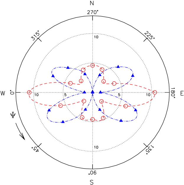
Figure 7: The East-West and North-South components of the field strength $|{\cal E}_{\nu EW}|$ and $|{\cal E}_{\nu NS}|$ (circles and triangles, respectively) at 55 MHz as functions of angle $\psi$ between the magnetic West and direction to the shower core. The distance between the origin and a circle or a triangle represents the field strength in the units of $\mu$V/m/MHz. The angular spacing between circles or triangles is $\pi/8$. At $\psi=\pm\pi/2$ $|{\cal E}_{\nu NS}|$ do not exceed 0.1 $\mu$V/m/MHz and two triangles overlap. All points were calculated for the vertical shower at a 200 m distance from the antenna.

The unusually high value of ${\cal E}_{\nu EW}$ at $\psi=0$ and $\pi$ can be explained when one takes a closer look at how the denominator of the second term of Eq. (1) changes as charged particles travel towards the Earth. As a positron starting from $(R,\psi=0,h)$ in cylindrical coordinates bends to the East, its velocity vector $\boldsymbol{\beta}$ becomes increasingly closer to the vector ${\bf n}$ towards the antenna. As a result, $1-n\boldsymbol{\beta}\cdot{\bf n}$ becomes smaller, the antenna gets closer to the Cherenkov cone defined as $1-n\boldsymbol{\beta}\cdot{\bf n}=0$ and the amplitude of the radio signal increases.

The same mechanism accounts for the fact that the signal at $\psi=\pi/8$ is larger than at $\psi=-\pi/8$. While bending around the Earth’s magnetic field ${\bf B}$, the originally vertical velocities of the charged particles do not just acquire an $x$-component. As a result of a nonzero dip angle $\gamma_{d}$ of the ${\bf B}$ field, both electron and positron velocities also get a small $y$-component towards the magnetic North as can be seen from Eqs. (8) and (12) below. This brings the velocity vector $\boldsymbol{\beta}$ of the positron starting at $\psi=\pi/8$ closer to the vector ${\bf n}$ towards the antenna. For the positron at $\psi=-\pi/8$ the situation is reversed. The North component of its velocity makes the angle between the velocity and direction to the antenna larger than it could have been without it. The third power in the denominator of the Eq. (1) amplifies the effect and the difference between signal amplitudes for these two angles becomes noticeable.

The symmetry of the plots with respect to the $Oy$ axis is remarkably good; the deviations between the corresponding values do not exceed 5%. Also, the field strengths ${\cal E}_{\nu NS}$ at $\psi=\pm\pi/2$ are very small compared to those at other angles. These results tend to improve with a higher statistics. The deviations between the symmetric dots become smaller and the NS components of the field strengths at $\psi=\pm\pi/2$ decrease even further. So, the deviations must be primarily statistical. Both features are in full accord with theoretical predictions (see Appendix).

VIII Conclusions

In this paper we presented a simple model of the cosmic ray air shower radio emission based on calculation of the trajectories and radiation of the charged particles of the shower maximum. Despite the limited nature of the model, it correctly predicts the order of magnitude of the radiation strength. We conclude that full scale shower development simulations can be appended with calculations of radiation from individual shower particles to give reliable predictions of the radiation properties. If the Auger arrays are equipped with antennas to detect the shower RF pulses, one would be able to check the model predictions for the showers with energies higher than $10^{20}$ eV.

As one can see from Fig. 7, the EW and NS components of the radio pulse are of the same order of magnitude and, hence, two perpendicularly oriented antennas should be deployed at future detector sites to get a full picture of shower radiation. The prominent superiority of the EW component over the NS one at $\psi=0,\,\pm\pi/2,\,\pi$ is quite sensitive to the value of the angle $\psi$. A future detector should accumulate a large sample of (almost) vertical showers before one would get radiation data from a few showers with cores directly to the North, South, East or West of the antenna. Then one should be able to confirm the conspicuous dominance of the EW component of their radiation over the NS one.

The polarization of the electromagnetic radiation is perpendicular to the direction of its propagation. For $10^{17}$ eV or weaker vertical showers with maximum mostly overhead, this means that the vertical component of the radiation is expected to be small. The relative strength of the vertical component is not small for inclined showers. Just like vertical showers, they radiate mostly in the direction of their development and a perpendicular to this direction may have an appreciable vertical component. However, inclined $10^{17}$ eV showers travel through a greater atmospheric thickness before they reach the ground and develop higher above the Earth. The overall strength of their radiation should be small. A greater penetration of very energetic ($\sim 10^{20}$ eV) inclined showers may compensate for this. In this case the shower radiation becomes stronger and the vertical component may become detectable. An additional vertically polarized antenna would facilitate the full measurement of the radiation from these most intense air showers.

Fig. 5 shows a strong dependence of pulse amplitude on the frequency. The optimal observation frequency band should be chosen with its lower limit at the lowest possible frequency consistent with a relatively small RF background (both natural and man-made), at around 20 or 30 MHz.

Appendix: Theory of electric field dependence on angle $\psi$

In the frame of Fig. 2 the Earth’s magnetic field vector ${\bf B}$ is parallel to the vector $(0,-\cos\gamma_{d},-\sin\gamma_{d})$, where $\gamma_{d}$ is the dip angle. The velocity vectors of electrons and positrons bend around it in opposite directions. A straightforward calculation gives the following expressions for position, velocity and acceleration of an electron:

$${\bf r}^{e}(t)=\left[R\cos\psi+\frac{\beta c\cos\gamma_{d}}{\omega}\,(1-\cos\omega t),\,R\sin\psi-\frac{\beta c\sin\gamma_{d}\cos\gamma_{d}}{\omega}\,\left(\omega t-\sin\omega t\right)\right.,$$

$$\left.h-\beta ct+\frac{\beta c\cos^{2}\gamma_{d}}{\omega}\,\left(\omega t-\sin\omega t\right)\right]\ ,$$ (7)

$${\bf v}^{e}(t)=\beta c\ \left[\cos\gamma_{d}\sin\omega t,\,-\sin\gamma_{d}\cos\gamma_{d}\,(1-\cos\omega t),\,-1+\cos^{2}\gamma_{d}\,(1-\cos\omega t)\right]\ ,$$ (8)

$${\bf a}^{e}(t)=\omega\beta c\cos\gamma_{d}\ (\cos\omega t,\,-\sin\gamma_{d}\sin\omega t,\,\cos\gamma_{d}\sin\omega t)\ ,$$ (9)

where

$$\omega=\frac{eB}{\gamma m}$$ (10)

is the gyration frequency and $t$ is the time in the observer’s frame. $t=0$ corresponds to the start of the particle motion. If the index of refraction $n$ were constant through the atmosphere depth, the relationship between the retarded time $t$ and the time $t_{a}$ when the signal arrives at the antenna would be $t_{a}=t+n\,|{\bf r}^{e}(t)|/c$. Time delays were corrected to take into account variations of the index of refraction with the altitude.

Similarly for a positron,

$${\bf r}^{p}(t)=\left[R\cos\psi-\frac{\beta c\cos\gamma_{d}}{\omega}\,(1-\cos\omega t),\,R\sin\psi-\frac{\beta c\sin\gamma_{d}\cos\gamma_{d}}{\omega}\,\left(\omega t-\sin\omega t\right)\right.,$$

$$\left.h-\beta ct+\frac{\beta c\cos^{2}\gamma_{d}}{\omega}\,\left(\omega t-\sin\omega t\right)\right]\ ,$$ (11)

$${\bf v}^{p}(t)=\beta c\ \left[-\cos\gamma_{d}\sin\omega t,\,-\sin\gamma_{d}\cos\gamma_{d}\,(1-\cos\omega t),\,-1+\cos^{2}\gamma_{d}\,(1-\cos\omega t)\right]\ ,$$ (12)

$${\bf a}^{p}(t)=\omega\beta c\cos\gamma_{d}\ (-\cos\omega t,\,-\sin\gamma_{d}\sin\omega t,\,\cos\gamma_{d}\sin\omega t).$$ (13)

The $|{\bf E}|$ independence of $\psi$ at $t=0$ [24] does not hold as electron-positron pairs travel towards the Earth. However, the symmetry does not break down completely. We will show below that the symmetry with respect to the $yOz$ plane remains, i.e., a pair starting from a point $(R,\psi,h)$ in cylindrical coordinates produces an electric field of the same magnitude as a symmetric pair from $(R,\pi-\psi,h)$.

First, note that a particle’s velocity and acceleration are obviously independent of $\psi$. For any time $t$ Eqs. (8), (9), (12), (13) give

$$\beta^{e}_{x}=-\beta^{p}_{x},\ \ \ \ \ \ \ \ \ \ \ \dot{\beta}^{e}_{x}=-\dot{\beta}^{p}_{x},$$ (14)

$$\beta^{e}_{y}=\beta^{p}_{y},\ \ \ \ \ \ \ \ \ \ \ \dot{\beta}^{e}_{y}=\dot{\beta}^{p}_{y},$$ (15)

$$\beta^{e}_{z}=\beta^{p}_{z},\ \ \ \ \ \ \ \ \ \ \ \dot{\beta}^{e}_{z}=\dot{\beta}^{p}_{z}.$$ (16)

Now, taking into account that ${\bf n}=-{\bf r}/r$, one can deduce from Eqs. (7) and (11) that for any time $t$

$$(n_{x})^{e}_{\psi}=-(n_{x})^{p}_{\pi-\psi},$$ (17)

$$(n_{y})^{e}_{\psi}=(n_{y})^{p}_{\pi-\psi},$$ (18)

$$(n_{z})^{e}_{\psi}=(n_{z})^{p}_{\pi-\psi}.$$ (19)

The above equations result in $(\boldsymbol{\beta}\cdot{\bf n})^{e}_{\psi}=(\boldsymbol{\beta}\cdot{\bf n})^{p}_{\pi-\psi}$, and the denominator of the second term in Eq. (1) is “CP symmetric”. As for the numerator, we rewrite the double vector product as ${\bf n}\,(\dot{\boldsymbol{\beta}}\cdot{\bf n})-n\boldsymbol{\beta}\,(\dot{\boldsymbol{\beta}}\cdot{\bf n})-\dot{\boldsymbol{\beta}}\,(1-n\boldsymbol{\beta}\cdot{\bf n})$. The expressions in parentheses are “CP symmetric”. As for vectors ${\bf n}$, $\boldsymbol{\beta}$ and $\dot{\boldsymbol{\beta}}$, the Eqs. (14-19) tell that their $y$ and $z$-components are “CP symmetric”, while the $x$-components are antisymmetric. Finally, take into account the opposite charge signs of positrons and electrons and obtain the following relations between the components of the electric field vectors:

$$(E_{x})^{e}_{\psi}=(E_{x})^{p}_{\pi-\psi},$$ (20)

$$(E_{y})^{e}_{\psi}=-(E_{y})^{p}_{\pi-\psi},$$ (21)

$$(E_{z})^{e}_{\psi}=-(E_{z})^{p}_{\pi-\psi}.$$ (22)

These relations can be directly translated to the case of two pancakes. Pancakes with centers at $(R,\psi,h)$ and $(R,\pi-\psi,h)$ contain symmetrically located electron-positron pairs. The $x$-components of the electric fields radiated by the pancakes and received at the antenna are the same and the $y$ and $z$-components only differ in sign. Thus, one expects a symmetry of the magnitude of any electric field component with respect to the $yOz$ plane.

One special case is a pancake at $\psi=\pi/2$ or $-\pi/2$. Each electron inside this pancake has a counterpart – a symmetrically located positron. This implies that $y$ and $z$-components of the pancake’s electric field vanish.

References

- [1] T. Abu-Zayyad et al., Astrophys. J. 557, 686 (2001).
- [2] J. Alvarez-Muniz and E. Zas, in Radio Detection of High Energy Particles (Proceedings of the First International Workshop RADHEP 2000), edited by D. Saltzberg and P. Gorham (AIP Conference Proceedings No. 579, AIP, New York, 2001), p. 117, astro-ph/0103369.
- [3] R. V. Buniy and J. P. Ralston, Phys. Rev. D 65, 016003 (2002).
- [4] P. Gorham et al., Phys. Rev. E 62, 8590 (2000).
- [5] D. Saltzberg et al., Phys. Rev. Lett. 86, 2802 (2001).
- [6] F. D. Kahn and I. Lerche, Proc. Roy. Soc. A 289, 206 (1966).
- [7] S. A. Colgate, J. Geophys. Res. 72, 4869 (1972).
- [8] H. R. Allan, in Progress in Elementary Particles and Cosmic Ray Physics, v. 10, edited by J. G. Wilson and S. G. Wouthuysen (North-Holland, Amsterdam, 1971), p. 171.
- [9] J. L. Rosner and D. A. Suprun, in Radio Detection of High Energy Particles [2], p. 81, astro-ph/0101089.
- [10] Radio Detection of High Energy Particles [2].
- [11] H. Falcke and P. Gorham, Astropart. Phys. 19, 477 (2003).
- [12] J. D. Jackson, Classical Electrodynamics, 3rd edition (Wiley, 1999), p. 664.
- [13] E. Zas, F. Halzen and T. Stanev, Phys. Rev. D 45, 362 (1992).
- [14] J. A. Wheeler and R. P. Feynman, Rev. Mod. Phys. 21, 425 (1949).
- [15] J. H. Hough, J. Phys. A 6, 892 (1973).
- [16] V. B. Atrashkevich et al., Yad. Fiz. 28, 712 (1978) [Sov. J. Nucl. Phys. 28, 366 (1978)].
- [17] T. K. Gaisser and T. Stanev, mini-review in Particle Data Group, K. Hagiwara et al., Phys. Rev. D 66, 010001 (2002), pp. 182–188.
- [18] M. F. Bourdeau, J. N. Capdevielle and J. Procureur, J. Phys. G 6, 901 (1980).
- [19] K. Greisen, Prog. Cosmic Ray Physics., Suppl. 3 (1956).
- [20] K. Kamata and J. Nishimura, Prog. Theor. Phys. Suppl. 6, 93 (1958).
- [21] J. Linsley, J. Phys. G 12, 51 (1986).
- [22] V. B. Atrashkevich et al., J. Phys. G 23, 237 (1997).
- [23] C. L. Pryke, Astropart. Phys. 14, 319 (2001).
- [24] K. Green, J. L. Rosner, D. A. Suprun and J. F. Wilkerson, Nucl. Instr. Meth. A 498, 256 (2003).
- [25] H. R. Allan, Proc. ICRC-11, Budapest, 1969, Invited Papers and Rapporteur Talks, p. 553; W. N. Charman, Nuovo Cimento Lett. 3, 845 (1970).