The optical light curves of XTE J2123–058: the mass of the binary components and the structure of the quiescent accretion disk

Abstract

We present optical photometry of XTE J2123–058 during its quiescent state taken in 1999 and 2000. The dominant feature of our R-band light curve is the ellipsoidal modulation of the secondary star, however, in order to fit this satisfactorily we require additional components which comprise an X-ray heated Roche-lobe filling secondary star, and an accretion disk bulge, i.e. where the gas stream impacts the accretion disk. The observed dip near phase 0.8 is interpreted as the eclipse of inner parts of the accretion disk by the bulge. This scenario is highly plausible given the high binary inclination. Our fits allow us to constrain the size of the quiescent accretion disk to lie in the range 0.26–0.56 $R_{\rm L1}$ (68 percent confidence). Using the distance of 9.6 kpc and the X-ray flux inferred from the heated hemisphere of the companion, we obtain an unabsorbed X-ray luminosity of 1.2$\times 10^{33}$ erg s^-1 for XTE J2123–058 in quiescence. From the observed quiescent optical/IR colors we find that the power-law index (-1.4) for the spectral distribution of the accretion disk compares well with other quiescent X-ray transients.

We also re-analyse the optical light curves of the soft X-ray transient XTE J2123–058 taken during its outburst and decay in 1998. We use a robust method to fit the data using a refined X-ray binary model. The model computes the light arising from a Roche-lobe filling star and flared accretion disk irradiated by X-rays, and calculates the effects of shadowing and mutual star/disk eclipses. We obtain relatively accurate values for the binary inclination and mass ratio, which when combined with spectroscopic results obtained in paper II gives a neutron star mass in the range 1.04–1.56 $M_{\odot}$ (68% confidence).

1 Introduction

Soft X-ray transients (SXTs), or X-ray novae in quiescence provide outstanding opportunities to study the mass donor and/or quiescent accretion disk in these low-mass X-ray binaries (LMXBs) because of the absence of the enormous glare that results from X-ray heated material during outburst. The majority of these systems appear to contain black-hole compact objects (see e.g. Charles 2001 and references therein), but four of them have been identified with neutron stars as a result of the typei X-ray bursts seen during X-ray active phases. The rarity of neutron star transients has been explained by King, Kolb Burderi (1996) as due to the effects of X-ray irradiation which can stabilize the accretion disk.

Furthermore, detailed studies of many transients are hampered by galactic extinction, as most lie in or close to the galactic plane. And, as yet, no transient has been seen to produce X-ray eclipses which would provide incontrovertible constraints on its orbital inclination. For these reasons, the recent SXT XTE J2123-058 is a system of considerable importance in this field. It is at high galactic latitude ($b_{\textsc{ii}}\sim$-36.2^∘), and during outburst (Zurita et al., 2000; hereafter paper I) displayed a dramatic optical modulation (the largest in this class of objects) which indicated that, even though not eclipsing, the inclination must be very high. Observations of typei bursts at optical (Tomsick, 1998b) and X-ray wavelengths (Takeshima & Strohmayer, 1998) indicated that the compact object is a neutron star, making it one of only four neutron star X-ray transients.

This paper is a companion to Casares et al., (2001; hereafter paper II) which presents the first spectroscopic detection of the companion in quiescence. Low resolution spectroscopy of XTE J2123-058 during its quiescent state revealed a K7v star with a radial velocity semi-amplitude of 287$\pm$12 km s^-1. Combined with the orbital period this implies a binary mass function of $f(M)$=0.61$\pm$0.08 M_⊙ (paper II). From these, estimates of the component masses were made, but it is clear that these are limited by the accuracy of the $q$ and $i$ values.

We present the optical light curve of XTE J2123–058 taken when the source was in quiescence. We model the multi-component optical light curves in terms of the light arising from an X-ray heated Roche-lobe filling secondary star, the accretion disk and the self eclipse of the inner part of the disk by the stream/disk impact region. We also take the opportunity to re-analyse the outburst and decay optical light curves of XTE J2123–058. The model we used previously suffered from computational biases, in particular when calculating eclipses. Also, as is the case in most fitting procedures, the best fit solution depends somewhat on the starting parameters. Here, we use a genetic-type algorithm which is more robust than conventional techniques, which allows us to determine accurate masses for the binary components.

2 Observations and data reduction

Cousin R-band CCD images of XTE J2123–058 in quiescence were obtained with the NTT 3.5m telescope on La Silla, the Bok 2.3-m telescope at the Steward Observatory, Arizona and with the WHT 4.2m telescope on La Palma between 1999 and 2000 (see Table 1 for details). Johnson UBV and Cousin RI observations were also obtained with the 4.2m WHT and INT 2.5m telescopes. In addition infrared (JHK) observations were obtained during September 1999 as part of the UKIRT Service Programme.

All the optical images were corrected for bias and flat-fielded in the standard way. The infrared images were dark-current subtracted and then flat-fielded using a median stack of the images. We applied profile-fitting photometry to our object and several nearby comparison stars within the field of view, using iraf. All the images were flux calibrated except for the J-band, because of the non-photometric conditions during the J-band standard star observations.

3 The colors of the accretion disk

We use the dereddened optical and infrared colors of XTE J2123–058 to recover the broad-band spectrum of the accretion disk by subtracting the companion star. We use a $\tt PHOENIX$ model atmosphere (Hauschildt, Allard & Baron, 1999) with $T_{\rm eff}$=4250 K and $\log g$=4.5 to represent the K7v secondary star, which is consistent with the spectral type classifaction by Tomisck et al., (2001). The observed mean colors and dates are given in Table 2. We first convolved the model atmosphere spectrum with the optical and infrared filter responses and then fixed the secondary star to contribute 77 percent of the observed flux at $\sim$6300Å (as determined in paper II). By subtracting the resulting colors from the observed dereddened colors of XTE J2123–058 based on $E_{\rm B-V}=0.12$ (Hynes et al.,, 2001) we obtain the colors of the accretion disk (see Figure 1). We find that the spectrum of the accretion disk can be represented by a power-law of the form $F_{\lambda}\propto\lambda^{n}$ with index -1.4.

If we use $T_{\rm eff}$=4500 K to represent a K5 secondary star, we obtain an exponent of -1.1. Changing the secondary star’s contribution to 70 percent increases the exponent by 0.3. Therefore we estimate a systematic uncertainty of $\pm$0.3. Since the optical and infrared observations were taken at different times we have to assume that the mean brightness of the source does not vary with time. Ideally we would like to determine the phase averaged magnitudes. Although most of our measurements do not cover a complete orbital cycle we believe that the large uncertainties in the measurement for each band are such that we allow for this systematic effect in our error estimate. The power-law index for the spectral distribution of the accretion disk compares well with that derived in other quiescent SXTs. In A0620–00 and Cen X–4 the power-law index is -2.5$\pm$1.0 (McClintock & Remillard, 1986) and -1.6$\pm$0.30 (Shahbaz, Naylor & Charles, 1998) respectively.

4 A re-analysis of the outburst/decay data

In this section we re-fit the optical light curves of XTE J2123–58 presented in paper I. The model that was originally used (paper I) suffered from many computational biases, the result of many transfers of the code to different operating systems which resulted in the miss-calculation of eclipses. The errors in the code were noticed when we tried to produce simple images of the binary system. Also, the code was not general and could only be used for systems with relatvely hot secondary stars as is the case in high-mass X-ray binaries (Tjemkes, Zuiderwijk & van Paradijs et al.,, 1986) and so it used Kurucz model atmospheres with temperatures hotter than 5500 K. Therefore we took the opportunity to write and fully test a new code that models the light from an X-ray irradiated Roche-lobe filling star and accretion disk orbiting a compact object. The model includes a flared accretion disk, and new model atmosphere fluxes and limb-darkening coefficients for cool stars. Also, we now use a robust genetic-type algorithm (Storn & Price, 1995) to fit the light curves. Unlike the algorithm used in paper I and most other studies, Genetic codes have been used before in fitting light curves, as in Metcalfe (1999), Gelino, Harrison & Orosz (2001) and Orosz et al., (2002), the best fit solution does not depend on the starting parameters. Hence we are able to improve on the accuracy of the mass determination for the binary components of XTE J2123–058.

4.1 The X-ray binary model

To interpret the optical light curves, we used a model that includes a Roche-lobe filling secondary star, the effects of X-ray heating on the secondary, a concave accretion disk, shadowing of the secondary star by the disk, and mutual eclipses of the disk and secondary star . For details of the model see Tjemkes, Zuiderwijk & van Paradijs et al., (1986) and Orosz & Bailyn (1997). The geometry of the binary system is given by the orbital inclination $i$, the mass ratio ($q=M_{2}/M_{1}$, where $M_{1}$ and $M_{2}$ are the masses of the compact object and secondary star respectively) and the Roche-lobe filling factor $f$ of the secondary star. The light from the secondary star is given by its mean effective temperature $\bar{T_{\rm eff}}$, the gravity darkening exponent $\beta$ and the X-ray albedo $W$. The temperature across the star is scaled such that it weighted mean matches the observed temperature. The light from the accretion disk is given by its radius $R_{\rm disk}$, defined as a fraction of the distance to the inner Lagrangian point ($R_{\rm L1}$), its flaring angle, $\alpha$, the temperature at the outer edge of the disk $T_{\rm out}$ and the exponent on the power-law radial temperature distribution $\xi$. Finally, the additional light due to X-ray heating is given by the unabsorbed X-ray flux $F_{X,0}$, the distance to the source $d_{\rm kpc}$ and the orbital separation (determined from the optical mass function $f(M)$, $P_{\rm orb}$ the $q$ and $i$.). The X-ray heating of the secondary star is computed in the same way as described by Tjemkes, Zuiderwijk & van Paradijs et al., (1986). We assume that the secondary is in synchronous rotation and completely fills its Roche lobe. Since the late-type secondary star has a convective envelope, we fix the gravity darkening exponent to 0.08 (Lucy, 1967). The albedo of the companion star ($W$) is fixed at 0.40 (de Jong, van Paradijs & Augusteijn, 1996). For ease, the key variables are listed in Table 3.

4.1.1 The accretion disk

The model assumes a flared, concave accretion disk of the form $h\propto r^{9/7}$ with $h$ and $r$ the disk height and radius respectively (Vrtilek et al.,, 1990). The radial distribution of the temperature across the disk is given by $T(r)=T_{\rm out}r^{\xi}$. For a steady-state, optically thick, viscous accretion disk, the exponent of the power-law is -3/4 (Pringle, 1981). For a disk heated by a central source the exponent is -3/7 (Vrtilek et al.,, 1990). The temperature of the accretion disk’s rim is fixed at $T_{\rm out}$. We assume that the disk radiates as a blackbody. For a given local temperature in the accretion disk, we calculate the blackbody intensity over the wavelength range of the filter and then convolve it with the response of the filter.

4.1.2 The intensity distribution

The intensity distribution on the secondary star is calculated using $\tt PHOENIX$ model atmospheres colors that are publically available on the World Wide Web. $\tt PHOENIX$ is a multi-purpose state-of-the-art stellar atmosphere code that can calculate atmospheres and spectra of stars all across the Hertzsprung-Russell diagram (Hauschildt, Allard & Baron, 1999). The colors that are available cover a range of temperatures (1700 K–30000 K) and gravity ($\log g$=3.5–5.0) and wavelength, and have been already convolved with standard filter responses. For this code to be of general use, it is important that one can calculate model atmospheres for cool stars. In order to accurately calculate the intensity at each grid point on the star, which depends on the local temperature and gravity, we use a 2–D bicubic spine interpolation method (Press et al.,, 1992) using the 2–D color grid.

We use a quadratic limb-darkening law to correct the intensity from the star and accretion disk. The coefficients are taken from Claret (1998) which were computed using $\tt PHOENIX$ model atmospheres. These calculations extend the range of effective temperatures 2000 K–50000 K and gravity $\log g$ = 3.5–5.0. Again we use a 2–D bicubic spline interpolation method to calculate the coefficients for a given temperature and gravity.

4.2 The fitting algorithm

The minimization of a function is a difficult one, especially if the function is complicated and has many parameters that are correlated and even more so if there are many isolated local minima or more complicated topologies. Methods such as Powell (a maximum-gradient technique), downhill simplex (polyhedral search technique) are only good if the global minimum lies near the initial guess values; this is not normally the case for complicated functions. When the objective function is nonlinear, direct search methods using algorithms such as by Nelder & Mead (1965) or genetic algorithms are the best approaches (Press et al.,, 1992).

The basic strategy at the core of every direct search method is to generate variations of the parameter vectors and make a decision whether or not to accept the newly derived parameters. A new parameter vector is accepted if and only if it reduces the value of the objective function. Although this process converges fairly fast, it runs the risk of becoming trapped by a local minimum. Inherently parallel search techniques like genetic and evolutionary algorithms have some built-in safeguards to ensure convergence. By running several vectors simultaneously, strong parameter configurations can help other vectors escape local minima.

Ideally an optimization technique should find the true global minimum, regardless of the initial system parameter values and should be fast. Storn & Price (1995) have developed a genetic-type technique called “Differential Evolution” , which is robust and simple. Differential Evolution generates new parameter vectors by adding the weighted difference vector between two population members to a third member. If the resulting vector yields a lower objective function value than a predetermined population member, the newly generated vector replaces the vector with which it was compared, in the next generation. The best parameter vector is also evaluated for every generation in order to keep track of the progress that is made during the minimization process. There are four main parameters in the differential evolution code; $\tt NP$, the number of population members (usually taken as 10$\times$ the number of fitting parameters); $\tt F$ the mutation scaling factor which controls the amplification of the difference vector; $\tt CR$ the crossover probability constant and $\tt itermax$, the maximum number of generations. For our problem of minimizing the $\chi^{2}$ function we use $\tt CR$=0.9, $\tt FX$=0.9 and $\tt itermax$=2000, which corresponds to $\sim$100,000 calculations of the function.

4.3 Fitting the outburst/decay data

We use the differential evolution algorithm described in section 4.2 to fit the same phase-binned outburst and decay light curves of XTE J2123–058 which were presented in paper I. We fix $d_{\rm kpc}$=9.6, $P_{\rm orb}$=0.2482 d and $\bar{T_{\rm eff}}$=4250 K corresponding to a K7 star (paper II). The observed X-ray flux (ASM 2–12 keV energy range) during the time of the outburst and decay data sets was 1.7$\times~{}10^{-9}$ erg cm^-2 s^-1 and 1.7$\times~{}10^{-10}$ erg cm^-2 s^-1 respectively. The R-band reddening is fixed to be 0.27 mags based on $E_{\rm B-V}=0.12$ (Hynes et al.,, 2001). The model parameters that we fit are $q$, $i$, $R_{\rm disk}$, $\alpha$, $T_{\rm out}$ and $\xi$.

For the outburst light curve with 29 data points we find a minimum reduced $\chi^{2}$, $\chi^{2}_{\nu}$ of 0.9 at $q=0.36$, $i$=72.5^∘, $R_{\rm disk}=0.69\,~{}R_{\rm L1}$, $\alpha$=5.9^∘, $\xi=-1.26$ and T${}_{\rm out}=2.5\times 10^{4}$  K. In order to determine the uncertainty in the parameters of interest we perform a 1–D grid search and plot the 68 percent and 90 percent confidence levels (see Table 4 and Figure 2). If we use a distance of $d_{\rm kpc}$=11 the minimum $\chi^{2}$ is not significantly different (at the 90 percent level). The inclination is the same, however, $\alpha$ increases by 3.5^∘. This is becasue the model needs to increase $\alpha$ in order to shield the secondary star from the strong X-ray heating (L_X=2.5$\times 10^{33}$ erg s^-1 for $d_{\rm kpc}$=11.0 compared with L_X=1.9$\times 10^{33}$ erg s^-1 for $d_{\rm kpc}$=9.6).

Since the quality of the outburst light curve is much better than the decay light curve, the eclipse features at orbital phases 0.0 and 0.5 are more evident. Hence, the parameters derived from modelling the outburst light curve will be more accurate compared to those derived from the decay light curve. Therefore for the decay light curve with 20 data points we fix $i$ and $q$ derived from the outburst light curve, and determine $R_{\rm disk}$ and $\alpha$ of the accretion disk. We find a minimum $\chi^{2}_{\nu}$ of 1.5 at $R_{\rm disk}=0.56\,~{}R_{\rm L1}$, $\alpha$=5.2^∘, $\xi=-1.19$ and T_out=7505  K (see Table 4). The best model fits to the outburst and decay light curves are shown in Figures 3 and  4 respectively. We also show the different components of light in the model, i.e. the accretion disk, the rim of the disk and the X-ray heated secondary star. It should be noted that changing $\bar{T_{\rm eff}}$ does not have a significant effect on the light curves; its effect is only significant at the 0.4 percent level. This is because of the dominant effect of X-ray heating. Changing the albedo of the companion star to 0.30 and 0.5 (de Jong, van Paradijs & Augusteijn 1996; Milgrom & Salpeter 1975) gives a worse $\chi^{2}$, but it is only significantly different at the 95 percent level. The derived parameters are the same within the uncertainties.

We can compare the results we obtained from fitting the outburst and decay light curves with our new model and fitting procedure with the those obtained in paper I. The outburst values obtained for $i$ and $\alpha$ in paper I were significantly overestimated (99% confidence level) compared to those we obtain here. Also, the value we obtain for $q$ in paper I was significantly underestimated ($>$99% level) compared to the value given here. The results obtained through fitting the decay light curve agree well with those obtained in paper I. The difference in the results compared to paper I is due mostly to the errors in the code and also in the fitting method used to find the global minimum solution (see section 4). The most likely reason why the results from the decay light curve are comparable is the relatively large error bars of the decay light curve. This would naturally give larger uncertainties in the derived parameters and so it is not surprising that the results obtained using the model in paper I and our new model agree.

Vrtilek et al., (1990) showed that the temperature profile of a flared accretion disk totally dominated by irradiation (i.e. isothermal) takes the form $T(r)\propto r^{-3/7}$ rather than $T(r)\propto r^{-3/4}$ for a steady-state non-irradiated disk. The value for the temperature exponent we derive is more negative ($\sim-1.2$) than either of these values. For a fixed outer disk temperature (and geometry) a steeper exponent implies a hotter disk. Therefore in order to match the observed flux using $\xi=-3/7$, the projected area of the disk in the outer parts must be on the whole smaller. Note that this can be achieved if the disk’s structure is warped; it has been known for some time that X-ray binaries can produce warped accretion disks (Wijers & Pringle 1999; Ogilvie & Dubus 2001). In order to explain the observed reprocessed X-ray flux in LMXBs, the disk in these systems must be either warped or the central X-ray source is not point like (Dubus et al.,, 1999). With this dataset we cannot determine the shape of the accretion disk. However, it should be noted that multi-color observations throughout an outburst may allow one to determine $\xi$ (see Orosz & Bailyn 1997) and more importantly provide information on the shape of the accretion disk in an SXT during outburst.

4.4 The shape of the light curves

At the start of an outburst angular momentum in the disk is transferred to the outer parts and so the matter diffuses inwards and the disk radius expands. When the system’s brightness decays, the disk shrinks in radius. The changes observed in the light curves during decline are primarily caused by large changes in the disk size and geometry. As we can see from the different component fits to the outburst and decay data, in outburst, the irradiated disk light swamps the light from the irradiated secondary star and hence the amplitude of the light curve is relatively small. As the irradiation of the disk becomes less the disk temperature is much cooler and the disk radius smaller, so the fraction of light from the disk is small compared to the fraction of light from the secondary star. This results in a large amplitude for the light curve. The triangular shaped minimum at phase 0.0 in the outburst light curve can be interpreted as the eclipse of the accretion disk by the X-ray heated secondary star. The deep mimimum in the outburst data at phase 0.5 i.e. when the X-ray heated secondary star is eclipsed by the disk, implies a larger disk radius compared to the disk radius when the X-ray irradiation is less. The same is true for the eclipse features at phase 0.0. The fit to the decay data requires a smaller and cooler, but not significantly thinner, accretion disk compared to the disk in the outburst data. Our model fits imply a change of $\sim$20 percent in the disk size.

5 The binary masses

The masses of the binary components are given by re-arranging the equation for the optical mass function,

$$M_{1}=\frac{K^{3}_{2}P_{\rm orb}}{2\pi G}\frac{(1+q)^{2}}{\sin^{3}i}~{}~{}M_{\odot};~{}~{}~{}~{}~{}~{}M_{2}=qM_{1},$$ (1)

where $K_{2}$ is the radial velocity semi-amplitude and $G$ is the Gravitational constant. Substituting our values for $q$ and $i$ with $K_{2}$ and $P_{\rm orb}$ we calculate $M_{\rm 1}$ and $M_{\rm 2}$. In order to determine the uncertainties we use a Monte Carlo simulation, in which we draw random values for the observed quantities which follow a given distribution, with mean and variance the same as the observed values. For $K_{2}$ and $P_{\rm orb}$ the random distribution are taken to be Gaussian because the uncertainties are symmetric about the mean value; $K_{2}$=287$\pm$12 km s^-1, $P_{\rm orb}$=0.248236$\pm$0.000002 days(1-$\sigma$ errors; paper II). However, for $q$ and $i$ the uncertainties are asymmetric and so we determine the actual distribution numerically. This is done by first calculating the maximum likelihood distribution using the actual $\chi^{2}$ fit values (see section 4.2) and then determining the cumulative probability distribution. By picking random values (from a uniform distribution) for the probability, we obtain random values for $q$ and $i$. Figure 5 shows the results of the Monte Carlo with 10⁶ simulations. Table 5 gives the ranges we obtain for the system parameters.

Tomisck et al., (2001) constrain the spectral type of the secondary star to lie in the range K5–K9. We can use the earliest spectral type (K5) for the secondary star to place an upper limit to the mass of the secondary star, since the mass of the secondary must be less than or equal to the main sequence mass of the same spectral type. A K5V star has a mass of ZAMS mass of 0.68 $M_{\odot}$ (Gray, 1992). Although the present-day mass of the secondary star is lower, and the secondary star is metal poor and hence will have a lower mass compared to a normal star, we can still use the ZAMS mass as a firm upper limit to the mass of the secondary star. Using this limit we constrain $M_{\rm 1}$ to lie in the range 1.04–1.56 $M_{\odot}$ and 0.95–1.68 $M_{\odot}$ (68% and 90% confidence respectively), which is consistent with the mass range determined in paper II and by Tomisck et al., (2001).

6 The quiescent light curve of XTE J2123–058

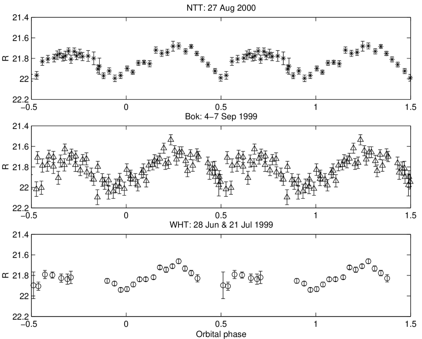
Figure 6: The observed quiescent R-band light curves of XTE J2123–058. From top to bottom: the NTT (August 2000), Bok (September 1999) and WHT (June/July 1999) data respectively. Note the stability of the light curves from epoch to epoch. For clarity 1.5 orbital cycles are shown.

In Figure 6 we show our new quiescent optical light curve of XTE J2123–058 obtained at different times, phase folded using the ephemeris given in paper II. Overall, the shape and mean brightness level of the light curves are very similar for data taken at three different epochs over a year. This is in contrast to the optical light curve of other SXTs, e.g. Cen X–4 and A0620–00 whose light curves are known to change shape and mean brightness (McClintock & Remillard 1990; Leibowitz, Hemar & Orio 1998; Gelino, Harrison & Orosz 2001). Such changes have been attributed to dark spots on the surface of the late-type companion star, which are thought to migrate on timescales of a few months to years (Bouvier & Bertout, 1998).

One expects the quiescent light curves of X-ray transients to be dominated by the ellipsoidal variations of the secondary star, which gives rise to a double-humped modulation, where the maxima are equal and the minima are unequal for high inclination systems. However, the quiescent light curve of XTE J2123–058 is far from being clean; the minumum at phase 0.0 (inferior conjunction of the secondary star) appears to be offset by $\sim$0.04 in phase. In an attempt to try and understand this light curve we consider two cases: (a) where we match the amplitude of the light curve between phase 0.0 and 0.5 and (b) where we match the light curve between phase 0.5 and 1.0 with our X-ray binary model (see Figure 7).

From the residuals for these two cases we can see that there is either excess light around phase 0.15 [case (a)] or there is a lack of light i.e. a dip around phase 0.8 [case (b)]. The excess light near phase 0.15 does not coincide with where a bulge is expected i.e the region where the gas-stream impacts the edge of the accretion disk; bright spots normally precede the secondary star and are observed around orbital phase $\sim$0.8–0.9 [see Wood et al., (1986) and Wood et al., (1989) for examples of the bright spot in high mass ratio quiescent dwarf novae]. Given the high binary inclination of XTE J2123–058 one can envisage situations where the inner part of the accretion disk is eclipsed by a bulge. If the bulge itself does not emit much light compared to the accretion disk, then the net effect on the light curves would be a decrease in light near phase 0.8. Similar effects have been seen in the UV light curves of Z Cha during superoutburst. In Z Cha the dip at phase 0.8 was explained as being due to vertical disk structure occulting the hot innner disk (Harlaftis et al.,, 1992). Therefore, in the next section we assume that the dip near phase 0.8 is due to the bulge eclipsing the inner parts of the accretion disk.

6.1 Fitting the quiescent light curve

The three quiescent R-band light curves of XTE J2123–058 were combined and binned into 30 phase bins. The parameters in the X-ray binary model that we vary are $i$, $\bar{T_{\rm eff}}$, $F_{\rm X,0}$, $R_{\rm disk}$, $T_{\rm out}$ and $\xi$. We fix $d_{\rm kpc}$=9.6 and the R-band reddening to be 0.27 mags. In our initial fits we let $\alpha$ run as a free parameter but we found that it did not make a significant difference to the fits (in fact an F-test on the best fit values does not justify the addition of an extra parameter), therefore we fixed its value to 2^∘, i.e. we assume a geometrically thin accretion disk. Given the determination of the veiling of the R-band light, we impose the condition that the accretion disk cannot contribute more than 33 percent to the observed light (using the upper limit of 77% for the secondary star’s contribution to the obseved flux; see paper II). When one determines the veiling of an absorption line spectrum, one compares the strength of the absorption lines of a template star (which normally has solar metalicity) with the target spectrum. If the target has a metal-poor spectrum, then the veiling will be overestimated. Given the high galactic latitude and systemic velocity of XTE J2123–058, the possibility that it is a halo metal poor system cannot be ruled out. Hence we use the veiling estimated in paper II as a firm upper limit to allow for the possibility that the veiling may be overestimated. We do not attempt to include an accretion disk bulge in the X-ray binary model because the height and temperature of the bulge most probably varies with orbital phase, thus introducing many parameters that would be difficult to deconvolve. Instead we model the accretion disk light eclipsed by the bulge as a gaussian function which is included in the fitting algorithm.

We use the differential evolution algorithm (see section 4.2) to fit the phase-binned light curve. For the fits with $q$=0.36, we find a minimum $\chi^{2}_{\nu}$ of 1.2 at $i$=71.8^∘, $\bar{T_{\rm eff}}=4610$ K, T${}_{\rm disk}=1425$ K, $R_{\rm disk}=0.45\,~{}R_{\rm L1}$, $\log F_{\rm X,0}$=-12.99 erg cm^-2 s^-1 and $\xi=-1.23$. The bulge is centered at 0.84$\pm$0.01 phase and has a gaussian width and height of 0.12$\pm$0.01 phase and -0.12$\pm$0.01 mags respectively. A 1–D grid search was performed to determine the uncertainties in the fitted parameters (see Table 6). For the fits with $q$=0.48, the minimum $\chi^{2}$ changes by less than 0.2 and the derived parameters are the same. The best model fit to the quiescent light curve and the different components in the model i.e. the accretion disk, the X-ray heated secondary star and the bulge, are shown in Figures 8 and 9 respectively. Changing the secondary star’s albedo to 0.3 and 0.5 does not change the $\chi^{2}$ of the fits significantly; the $\chi^{2}$ changes by only 0.05. Also, using an gravity darkening exponent of 0.10 does not change the fits; the $\chi^{2}$ changes by only 0.07. With the execption of $W$, within the uncertainties, the derived parameters are not different. For $W$=0.3 and 0.5 we obtain $\log F_{\rm X,0}$=-13.12 and -12.81 erg cm^-2 s^-1 respectively. Using the distance of 9.6 kpc and the X-ray flux obtained from the fits, we obtain an unabsorbed X-ray luminosity of 1.2$\times 10^{33}$ erg s^-1 for XTE J2123–058 in quiescence.

The binary inclination angle we obtain by fitting the quiescent light curve is similar to what was obtained by fitting the outburst data (see section 4.3) The value we obtain for $\bar{T_{\rm eff}}$ implies a K5 spectral type which is consistent (within the uncertainties), with the classification of the secondary star using the absorption lines (see paper II). To see if our interpretation of the disk bulge eclipse is correct we added a bulge to the accretion disk rim. To illustrate its effect we compute a model light curve which is shown in Figure 10. We fix the system parameters to the best fit values derived earlier. We varied the height of the bulge and the orbital phase range where it lies in order to match the observed light curve. The bulge was chosen to have a constant arbitrary height of 17^∘ (i.e. the flare angle at the edge of the disk) and constrained to lie between orbital phase 0.65 and 1.0. The temperature of the bulge is taken to be the same as the temperature of the disk’s edge. As one can see, the model clearly predicts less flux near phase 0.8, which is due to the eclipse of the X-ray heated disk by the cooler disk bulge.

7 Discussion

7.1 The accretion disk radius

We have measurements of the accretion disk radius in XTE J2123–058 at three different stages of its outburst; near the peak of outburst, during decay and in quiescence. The accretion disk radius we measure for XTE J2123–058 in quiescence is consistent with that measured in other SXTs. Although theoretically we cannot comment exactly on how the disk size changes with time, it should be noted that it is plausible that the disk radius decays exponentially as is inferred in dwarf novae (Smak, 1984).

7.2 The mass of the neutron star

Observationally, the mean mass of neutron stars in binary radio pulsars is $1.38\pm 0.07\,M_{\odot}$ (Thorsett & Chakrabarty, 1999). The models of Fryer & Kaolgera (2001) agrees well with this observed peak; they determined the neutron star and black hole initial mass function, and find that 81-96 percent of neutron stars lie in the mass range between 1.2–1.6 $M_{\odot}$. Within this framework the current mass of the neutron star in XTE J2123–058 (1.30 $M_{\odot}$; Table 5) may be the mass at its formation. However, in LMXBs, one expects massive neutrons stars to exist, because the neutron star has been accreting at the Eddington rate for a long period of time (Zhang et al.,, 1997). The observations of kilohertz quasi-periodic oscillations in some neutron star LMXBs, suggests that neutron stars could be as massive as $\sim 2\,M_{\odot}$. If the neutron stars in LMXBs are formed with a mass of $\sim 1.4\,M_{\odot}$, then it is quite possible to accrete an extra $\sim 0.6\,M_{\odot}$ in $\sim 10^{8}$ years (Zhang et al.,, 1997).

7.3 The secondary star and outburst mechanism

The transient behavior in LMXBs has been diskussed by King et al., (1996) and van Paradijs (1996). In the model of King et al., (1996), for a given magnetic braking law, the mass transfer rate is smaller in black hole X-ray binaries than in neutron star X-ray binaries. Short period neutron star X-ray binaries will only be transient if their companions are highly evolved, because the mass transfer rates in binaries with evolved companions are smaller than in systems with unevolved companions. A system will be transient if the average mass transfer rate ($-\dot{M_{2}}$) is smaller than some critical value ($\dot{M_{\rm crit}}$). Although we find $-\dot{M_{2}}/\dot{M_{\rm crit}}$ to be at least a factor of 4, obtained using our 90 percent mass limits for the binary components and the equations for $-\dot{M_{2}}$ and $\dot{M_{\rm crit}}$ given in King et al., (1996), there are many uncertainies in how the mass transfer rates are determined (see paper II); the magnetic braking mechanism is not very well understood (Kalogera, Kolb & King, 1998) and it could be that the mass transfer rate we see is not the secular mean. Also, XTE J2123–058 may have had a very different evolutionary path compared to other SXTs. The system may be a remnant of a thermal-timescale mass transfer, leading to peculiarities close to the end of the thermal phase (King private communication).

7.4 The X-ray heated secondary star

The H$\alpha$ doppler map of XTE J2123–058 in quiescence presented in paper II shows significant emission arising near the inner Lagrangian point, which could be due to the X-ray heating or chromospheric activity on the secondary star. Our fits require the inner face of the secondary star to be heated in order to match the observed shape of the minimum at phase 0.5. The dashed line in Figure 8 shows a model light curve with no X-ray heating. It has been known for some time that strong X-ray heating in an interacting binary can affect the form of the light curve (van Paradijs & McClintock, 1995). X-ray heating changes the photometric light curve by adding light to the minimum at phase 0.5 and changes the radial velocity curve by shifting the effective centre of the secondary, weighted by the strength of the absorption lines, from the centre of mass of the star, resulting in a significant distortion of the radial velocity curve.

The X-ray heating is such that the inner face of the secondary star is hotter than the outer face. We can estimate the expected change in temperature between the inner and outer faces of the secondary star. Using the X-ray binary model we computed the orbital variation in the (V-R) color of the secondary star with and without X-ray heating. We find the color difference between orbital phase 0.0 and 0.5 to be very small, 0.02 mags, which corresponds to a temperature change of only $\sim$60 K. Such a small temperature change would be very difficult to detect.

In order to investigate the effects of X-ray heating we computed the radial velocity of the secondary star using a crude treatment for X-ray heating (Phillips, Shahbaz & Podsiadlowski, 1999), where we impose the condition that if the incident flux from the X-ray source is more than 50 percent of the intrinsic flux from the secondary star then the absorption line flux is set to zero. Given the X-ray luminosity we estimate that such a level of irradiation will distort the radial velocity curve of the secondary star by $\sim$3 percent. However, given the faintness and hence the accuracy of the radial velocity curve, this effect would not be currently measurable.

The late-type companion stars in X-ray transients are perfect candidates to show chromospheric activity. This is because, these stars are tidally locked in short orbital periods and hence have rapid rotation rates. The chromospheric activity would be present in the form of narrow H$\alpha$ and Caii emission. Although Casares et al., (2001) detect H$\alpha$ emission at the inner Lagrangian point, it is difficult to say if this emission is solely due to chromospheric activity since the H$\alpha$ emission can also be powered by X-ray heating. However, we can ask how much of the H$\alpha$ emission can in principle be powered by X-ray heating. To do this we need to compare this predicted emission rate from the X-ray source with the observed H$\alpha$ photon emission rate.

The rate of emission of photons $N_{p}$ with a given energy is given by

$$N_{p}=\frac{F_{p}4\pi d^{2}}{E_{p}}$$ (2)

where $F_{\rm p}$ is the photon flux, $d$ is the distance to the source and $E_{\rm p}$ is the energy of the photon. From the H$\alpha$ Doppler map (paper II) we estimate the fractional contribution of the emission on the secondary star relative to the total H$\alpha$ emission. We then use this fraction with the equivalent width of the whole H$\alpha$ emission line to estimate the width of the narrow component, which we find to be $\sim$1Å. This combined with the dereddened R-band magnitude [$m_{R}$=21.8); E_B-V=0.12 (Hynes et al.,, 2001)] thus gives an H$\alpha$ flux photon flux of 1.7$\times 10^{-18}$ erg cm^-2 s^-1 which corresponds to an emission rate of $N_{\rm H\alpha}=4.1\times 10^{40}$ photon s^-1 ($d_{\rm kpc}$=9.6 and $E_{H\alpha}$=1.9eV).

In order to calculate the X-ray photon flux we assume that each X-ray photon causes one photoionisation of Hi and a fraction $\eta$ then recombine to produce an H$\alpha$ photon. The fraction is given by the ratio of the recombination rate of H$\alpha$ to the total recombination rate of Hi as a whole and is taken to be 0.45 for Case B recombination (Hummer & Storey, 1987). One also has to allow for the fact that only a fraction of the high energy photons actually cause photoionisation. This fraction $f_{\Omega}$, depends on the solid angle subtended by the secondary star and the accretion disk at the compact object, which is $\Omega_{\rm star}=\pi(R_{2}/a)^{2}$ (=0.28) for the star, whereas the planar disk which shields the secondary star subtends a solid angle of $\Omega_{\rm disk}=4(R_{d}/a)\tan\alpha$ (=0.04; where $R_{d}$ is the accretion disk and $a$ is the binary separation). Using these values we estimate $f_{\Omega}$=0.24. Finally one needs to allow for the X-ray albedo of the secondary star which is taken to be 0.4 (de Jong, van Paradijs & Augusteijn, 1996). Assuming that the inferred unabsorbed X-ray flux (see section 6.1) has a mean energy of 2 keV, a distance of 9.6 kpc and allowing for factors mentioned above, we obtain the the X-ray photon flux of $N_{\rm X-ray}=1.0\times 10^{41}$ photon s^-1. Since the predicted number of X-ray photons that produce H$\alpha$ photons is larger than the actual number observed, we conclude that the H$\alpha$ observed from/near the secondary star can in principle by powered by X-ray heating.

7.5 Comparison with other neutron star SXTs

The X-ray luminosity in quiescence we derived for XTE J2123–058 is comparable with that observed in other neutron star SXTs, typically 10^32-33 erg s^-1. Although there is some debate as to the origin of these quiescent X-rays, accretion seems to be the dominant source. Brown, Bildsten & Rutledge (1998) suggest that the X-rays could be due to cooling of the neutron star’s crust which is heated during outburst. However, as pointed out by Narayan, McClintock & Garcia (2001), neutron star SXTs have about half their total luminosity in their X-ray power-law tails, which is most likely to be produced by accretion rather than crustal cooling. Also, recent Chandra X-ray observations of Aql X–1 in quiescence show that the X-ray luminosity varies on timescales which are not consistent with the heated neutron star crust model (Rutledge et al.,, 2001). It should be noted that the observed X-ray flux in XTE J2123–058 is also too high to be due to the coronal emission from the companion. Following Bildsten & Rutledge (2000), we estimate the X-ray/bolometric flux ratio $F_{\rm X,0}/F_{\rm bol}$ to be 3.7, i.e. similar to what is observed in other quiescent neutron star SXTs.

Normally the X-ray luminosities of SXTs are obtained by direct X-ray observations of the source. Our optical study of XTE J2123–058 in quiescence has allowed us to infer the quiescent X-ray luminosity. What would be of great interest is a direct confirmation of the X-ray flux through direct measurements.

Table 1: Log of observations

Telescope	Date	Exposure time	Band
WHT 4.2m	28 Jun 1999	7$\times$530 s	R
WHT 4.2m	6 Jul 1999	157$\times$180 s	R
WHT 4.2m	7 Jul 1999	1$\times$600 s	I
WHT 4.2m	7 Jul 1999	1$\times$600 s	V
WHT 4.2m	7 Jul 1999	1$\times$1200 s	B
WHT 4.2m	21 Jul 1999	15$\times$600 s	R
Bok 2.3m	4–7 Sep 1999	68$\times$1200 s	R
UKIRT 3.5m	4 Sep 1999	36$\times$60 s	K
UKIRT 3.5m	6 Sep 1999	54$\times$60 s	J
UKIRT 3.5m	10 Sep 1999	54$\times$60 s	H
NTT 3.5m	27 Aug 2000	39$\times$600 s	R
INT 2.5m	5 Nov 2000	5$\times$1800 s	U
INT 2.5m	5 Nov 2000	1$\times$900 s	U
INT 2.5m	5 Nov 2000	1$\times$600 s	U
INT 2.5m	5 Nov 2000	1$\times$300 s	U

Table 2: Observed quiescent average magnitudes of XTE J2123–058

Band	Date	Observed magnitude	reddening∗
U	5 Nov 2000	23.68 $\pm$ 0.02	0.56
B	7 Jul 1999	23.75 $\pm$ 0.11	0.49
V	7 Jul 1999	22.65 $\pm$ 0.06	0.37
R	21 Jul 1999	21.81 $\pm$ 0.02	0.27
I	7 Jul 1999	21.08 $\pm$ 0.04	0.18
H	10 Sep 1999	19.48 $\pm$ 0.49	0.06
K	4 Sep 1999	19.98 $\pm$ 0.48	0.04

^∗ $A_{\rm V}/E_{\rm B-V}=3.1$; Howarth (1983) and Seaton (1979).

Table 3: A list of the key variables used in this paper and what they represent.

$M_{\rm 1}$	Mass of the compact object
$M_{\rm 2}$	Mass of the secondary star
$q$	Binary mass ratio defined as $M_{\rm 2}$/$M_{\rm 1}$
$i$	Binary inclination
$d_{\rm kpc}$	Distance
$P_{\rm orb}$	Orbital period
$K_{\rm 2}$	Secondary star’s radial velocity semi-amplitude
$\bar{T_{\rm eff}}$	Mean effective temperature of the seondary
$\beta$	Gravity darkening exponent
$W$	Albedo of the secondary star
$R_{\rm disk}$	Accretion disk radius
$\alpha$	Accretion disk flare angle
$T_{\rm out}$	Outer disk edge temperature
$\xi$	Exponent on the power-law radial temperature distribution
$F_{\rm X,0}$	Unabsorbed X-ray flux
$A_{\lambda}$	Interstellar reddening at a given wavelength $\lambda$

Table 4: Results obtained from the fits to the outburst and decay data

Paramter	Best fit	68% confidence	90% confidence
Outburst data
$q$	0.36	+0.01 $-$0.01	+0.16 $-$0.02
$i$ (∘)	72.5	+0.7 $-$0.7	+1.0 $-$2.3
$R_{\rm disk}$ ($R_{\rm RL1}$)	0.69	+0.01 $-$0.02	+0.03 $-$0.03
$\alpha$ (∘)	5.9	+0.2 $-$0.5	+0.5 $-$0.7
Decay data
$R_{\rm disk}$ ($R_{\rm RL1}$)	0.56	+0.03 $-$0.03	+0.05 $-$0.05
$\alpha$ (∘)	5.2	+0.5 $-$0.6	+0.9 $-$0.8

Table 5: Results of the Monte Carlo simulation: the binary masses

Paramter	Best fit	68% confidence	90% confidence
$M_{1}$ ($M_{\odot}$)	1.30	1.04 $-$1.70	0.95$-$1.92
$M_{2}$ ($M_{\odot}$)	0.46	0.36 $-$0.83	0.32 $-$0.98
$R_{2}$ ($M_{\odot}$)	0.59	0.54 $-$0.74	0.53 $-$0.76

Table 6: Results obtained from the fit to the quiescent data

Paramter	Best value	68% confidence	90% confidence
$i$	71.8	73.0 $-$69.0	73.5 $-$ 67.0
$R_{\rm disk}$ ($R_{\rm RL1}$)	0.45	0.24 $-$ 0.66	0.10 $-$ 0.80
$\bar{T_{\rm eff}}$ (K)	4610	4575 $-$ 4645	4560 $-$ 4680
$\xi$	-1.2	-1.5 $-$ -0.6	-1.8 $-$ -0.4
$\log F_{\rm X,0}$ ($\rm erg~{}cm^{-2}~{}s^{-1}$)	-12.99	-12.92 $-$ -13.08	-12.88 $-$ -13.17
$T_{\rm out}$ (K)	1425	300 $-$ 4000	$<$ 5000

Table 7: Accretion disk radius evolution

$\Delta t^{*}$ (days)	$R_{\rm disk}$ ($R_{\rm L1}$)	$\log F_{\rm X}$ ($erg~{}cm^{-2}~{}s^{-1}$)
29	0.69$\pm$0.02	-7.77
48	0.56$\pm$0.03	-8.77
551	0.45$\pm$0.21	-12.99

Figure 1: Top panel: the dereddened UBVRIHK colors of XTE J2123–058 are shown as crosses. The dotted line shows a $\tt PHEONIX$ model atmosphere spectrum of a K7v star scaled so that it contributes 77 percent to the R-band flux. Bottom panel: the spectrum of the accretion disk obtained by subtracting the filter-folded K7 star colors from the dereddened colors. The spectrum has a power-law shape with index -1.4.

Figure 2: The $\chi^{2}$ values obtained for the outburst data by grid searching the binary inclination (top panel) and mass ratio (bottom panel) whilst minimising the other model parameters. The dashed line shows the 90 percent confidence level.

Figure 3: Top panel: the average R-band orbital light curve during outburst (26–30 July 1998) of XTE J2123–058 (vertical line) and the best model fit (solid line). The vertical lines represent the error in the mean of each phase bin. Bottom panel: the three components in the X-ray binary model which gives the best fit to the outburst light curve. The accretion disk and rim are shown along with the X-ray heated secondary star and the total flux. For clarity 1.5 orbital cycles are shown.

Figure 4: Top panel: the average R-band orbital light curve during decay (16 Aug 1998) of XTE J2123–058 (vertical line) and the best model fit (solid line). The vertical lines represent the error in the mean of each phase bin. Bottom panel: the three components in the X-ray binary model which gives the best fit to the outburst data. The accretion disk and rim are shown along with the X-ray heated secondary star and the observed flux. For clarity 1.5 orbital cycles are shown.

Figure 5: The mass of the binary components obtained using a Monte Carlo simulation of the observed parameters and their uncertainties (see section 5). The 68 percent and 90 percent confidence levels are marked as the thin and thick lines respectively. The vertical line shows the mass of a ZAMS K5V star.

Figure 7: Top panel: Model fits for case (a) and case (b) (see text): middle and bottom panels are the residuals for case (b) and (a) respectively.

Figure 8: The observed quiescent R-band light curve of XTE J2123–058 (crosses) and the best model fit (sold line). The dashed lines show a model with no X-ray heating. For clarity 1.5 orbital cycles are show.

Figure 9: The separate components in the X-ray binary model which gives the best fit to the quiescent data. The accretion disk and bulge are shown along with the X-ray heated secondary star and the total observed flux. For clarity 1.5 orbital cycles and dereddened fluxes are shown.

Figure 10: The observed quiescent R-band light curve of XTE J2123–058 and a model light curve to show the effects of the accretion disk bulge. The solid line is a model light curve computed with the X-ray binary model with a bulge on the edge of the accretion disk. The bulge has a constant height of 17^∘ (the flare angle at the edge of the disk) and is confined to lie between orbital phase 0.65 and 1.0. The effect of the bulge is to eclipse the inner parts of the accretion disk, thus producing the dip near phase 0.8. For clarity 1.5 orbital cycles are shown.

References

- Bildsten & Rutledge (2000) Bildsten, L., & Rutledge, R. E., 2000, ApJ, 541, 908
- Bouvier & Bertout (1998) Bouvier, J., & Bertout, C., 1998, A&A, 211, 641
- Brown, Bildsten & Rutledge (1998) Brown, E.F., Bildsten, L., & Rutledge, R. E., 1998, ApJ, 504, 95
- Casares et al., (2001) Casares, J., Dubus, G., Shahbaz, T., Zurita, C., & Charles, P.A., 2002, MNRAS, 329, 29 (paper II)
- Claret (1998) Claret, A., 1998, A&A, 335, 647
- de Jong, van Paradijs & Augusteijn (1996) de Jong, J.A., van Paradijs, J., & Augusteijn, T., 1996, A&A, 314, 484
- Dubus et al., (1999) Dubus, G., Lasota, J-P., Hameury, J-M., & Charles, P.A., 1999, MNRAS, 303, 139
- Fryer & Kalogera (1999) Fryer, C., & Kalogera, V., 2001, ApJ, 554, 548
- Gelino, Harrison & Orosz (2001) Gelino, D.M., Harrison, T.E., & Orosz, J.A., 2001, AJ, 122, 2668
- Gray (1992) Gray, D.F., 1992, in The observation and analysis of stellar photospheres, Cambridge University Press, Cambridge, 430
- Harlaftis et al., (1992) Harlaftis, E.T., Hassall, B.J.M., Naylor, T., Charles, P.A., & Sonneborn, G., 1992, MNRAS, 257, 607
- Hauschildt, Allard & Baron (1999) Hauschildt, P.H., Allard, F., & Baron, E., 1999, ApJ, 512, 377
- Howarth (1983) Howarth, I.D., 1983, MNRAS, 203, 301
- Hummer & Storey (1987) Hummer, D.G., & Storey, M.J., 1987, MNRAS, 224, 801
- Hynes et al., (2001) Hynes, R.I., Charles, P.A., Haswell, C.A., Casares, J., Zurita, C., & Serra-Ricart, M., 2001, MNRAS, 324, 180
- Kalogera, Kolb & King (1998) Kalogera, V., Kolb, U., & King, A.R., 1998, ApJ, 504, 967
- King et al., (1996) King, A.R., Kolb, U., & Burderi, L., 1996, ApJ, 464, L127
- Leibowitz, Hemar & Orio (1998) Leibowitz, E.M., Hemar, S., & Orio, M., 1998, MNRAS, 300, 463
- Lucy (1967) Lucy, L.B., 1967, Zs. f. Ap. 65, 89
- McClintock & Remillard (1986) McClintock, J.E., & Remillard, R.A., 1986, ApJ, 308, 110
- McClintock & Remillard (1990) McClintock, J.E., & Remillard, R.A., 1990, ApJ, 350, 386
- Metcalfe (1999) Metcalfe, T.S., 1999, AJ, 117, 2503
- Milgrom & Salpeter (1975) Milgrom, M., & Salpeter, E.E., 1975, ApJ, 196, 583
- Narayan, McClintock & Garcia (2001) Narayan, R., Garcia, M.R., & McClintock, J.E., 2001, in Proc. IX Marcel Grossmann Meeting, eds. V. Gurzadyan, R. Jantzen and R. Ruffini, Singapore: World Scientific
- Nelder (1965) Nelder, J.A., & Mead, R., 1965, Computer Journal, Vol. 7, p 308
- Ogilvie & Dubus (2001) Ogilvie, G.I., & Dubus, G., 2001, MNRAS, 320, 485
- Orosz & Bailyn (1997) Orosz, J.E., & Bailyn, C., 1997, ApJ, 477, 876
- Orosz et al., (2002) Orosz, J.A., Groot, P.J., van der Klis, M.R., McClintock, J.E., Garcia, M.R., Zhao, P., Jain, R., Bailyn, C.D., & Remillard, R.A., 2002, ApJ, 568, 845
- Phillips, Shahbaz & Podsiadlowski (1999) Phillips, S.N., Shahbaz, T., & Podsiadlowski, Ph., 1999, MNRAS, 304, 839
- Press et al., (1992) Press, W.H., Teukolsky, S.A., Vetterling, V.T., & Flannery, B.P., 1992 in Numerical Recipes in Fortran, 2nd edition, Cambridge, Cambridge University Press
- Pringle (1981) Pringle, J.E., 1981, ARA&A, 19, 137
- Rutledge et al., (2001) Rutledge, R., Bildsten, L., Brown, E.F., Pavlov, G.G., & Zavlin, V., 2001, ApJ, 559, 1054
- Seaton (1979) Seaton, M.J., 1979, MNRAS, 187, 73
- Shahbaz, Naylor & Charles (1998) Shahbaz, T., Naylor, T., & Charles, P.A, 1993, MNRAS, 265, 655
- Smak (1984) Smak, J., 1984, AcA, 34, 93
- Soria, Wu & Galloway (1999) Soria, R., Wu, K., & Galloway, D.K., 1999, MNRAS, 309, 528
- Storn & Price (1995) Storn, R., & Price, K., 1995, Technical report TR-95-012
- Takeshima & Strohmayer (1998) Takeshima, T., & Strohmayer, T.E., 1998, IAC Circ. 6958
- Thorsett & Chakrabarty (1999) Thorsett, S., & Chakrabarty, D., 1999, ApJ, 512, 288
- Tomsick (1998b) Tomsick, J.A., Kemp, J., Halpern, J.P., & Hurley-Keller, D., 1998, IAU Circ. 6972
- Tomisck et al., (1999) Tomsick, J.A., Halpern, J.P., Kemp, J., & Kaaret, P., 1999, ApJ, 521, 341
- Tomisck et al., (2001) Tomsick, J.A., Heindl, W.A., Chakrabarty, D., Halpern, J.P., & Kaaret, P., 2001, ApJ, 559, L123
- Tjemkes, Zuiderwijk & van Paradijs et al., (1986) Tjemkes, S.A., Zuiderwijk, E.J., & van Paradijs, J., 1986, A&A, 154, 77
- van Paradijs & McClintock (1995) van Paradijs, J., & McClintock, J. E., 1995, in X-ray Binaries, eds. W.H.G. Lewin, J. van Paradijs and E.P.J. van den Heuvel, Cambridge, Cambridge University Press, p. 58.
- van Paradijs (1996) van Paradijs, J., 1996, ApJ, 464, L139
- Vrtilek et al., (1990) Vrtilek, S.D., Raymond, J.C., Garcia, M..R., Verbunt, F., Hasinger, G., & Kurster, M., 1990, A&A, 235, 162
- Wijers & Pringle (1999) Wijers, R.A.M., & Pringle, J.E., 1999, MNRAS, 308, 207
- Wood et al., (1986) Wood, J., Horne, K., Berriman, G., Wade, R.A., O’Donoghue, D., & Warner, B., 1986, MNRAS, 219, 629
- Wood et al., (1989) Wood, J., Horne, K., Berriman, G., & Wade, R.A., 1989, ApJ, 341, 974
- Zhang et al., (1997) Zhang, W., Strohmayer, T. E., & Swank, J. H., 1997, ApJ, 482, L167
- Zurita et al., (2001) Zurita, C., Casares, J., Shahbaz, T., Charles, P.A., Hynes, R.I., Shugarov, S., Goransky, V., Pavlenko, E.P., & Kuznetsova, Y., 2000, MNRAS, 316, 137, (paper I)