A new look at the pulsating DB white dwarf GD 358: Line-of-sight velocity measurements and constraints on model atmospheres

We report on our findings of the bright, pulsating, helium atmosphere white dwarf GD 358, based on time-resolved optical spectrophotometry. We identify 5 real pulsation modes and at least 6 combination modes at frequencies consistent with those found in previous observations. The measured Doppler shifts from our spectra show variations with amplitudes of up to 5.5 $\rm km\,s^{-1}$ at the frequencies inferred from the flux variations. We conclude that these are variations in the line-of-sight velocities associated with the pulsational motion. We use the observed flux and velocity amplitudes and phases to test theoretical predictions within the convective driving framework, and compare these with similar observations of the hydrogen atmosphere white dwarf pulsators (DAVs). The wavelength dependence of the fractional pulsation amplitudes (chromatic amplitudes) allows us to conclude that all five real modes share the same spherical degree, most likely, $\ell=1$. This is consistent with previous identifications based solely on photometry. We find that a high signal-to-noise mean spectrum on its own is not enough to determine the atmospheric parameters and that there are small but significant discrepancies between the observations and model atmospheres. The source of these remains to be identified. While we infer $T_{\mathrm{eff}}$$\thickspace=24$ kK and $\log g\sim 8.0$ from the mean spectrum, the chromatic amplitudes, which are a measure of the derivative of the flux with respect to the temperature, unambiguously favour a higher effective temperature, 27 kK, which is more in line with independent determinations from ultra-violet spectra.

1 Introduction

Given the potential for successful asteroseismology, pulsating white dwarfs have received considerable attention in recent years. However, this asteroseismological potential has only been tapped for a few objects partly due to a lack of understanding of the observed behaviour of the pulsations. Turning the problem around, the potential to gain insight into the the physics of the upper atmosphere of white dwarfs, using the pulsations themselves, is almost as great. This approach will ultimately elucidate the nature of the pulsations in a variety of ways.

White dwarfs can be broadly divided into two groups: those with atmospheres composed almost exclusively of hydrogen (DA types), and those with nearly pure helium atmosphere (DB types). The former comprise up to 80% of the total population of white dwarfs, while the latter dominate the remaining 20%.

Both groups of white dwarfs evolve through a phase of pulsational instability; the DB instabilty strip stretches from $\sim$ 27-22 kK, while that of the DAs ranges from $\sim$ 12.5-11.5 kK. Both are non-radial, g-mode pulsators (Chanmugam 1972; Warner & Robinson 1972), and typical pulsation periods are of the order of several hundred seconds. This evolutionary phase provides a window into the interiors of these objects.

How do the global properties of the pulsating DBs ($\equiv$ DBVs) compare with those of the better-studied DAVs? Do they follow the same trends across the instability strip? Are the same driving and amplitude saturation mechanisms at work?

The driving of the pulsations was originally thought to occur in an ionisation zone via the $\kappa$-mechanism i.e. in a manner akin to that of the Cepheids and $\delta$-Scuti type stars (e.g. Dziembowski & Koester 1981; Dolez & Vauclair 1981; Winget et al. 1982a). However, Brickhill (1983, 1991) realised that the convective turnover time is short ($\sim$ 1 s) compared with the mode periods, meaning that the convective zone can respond instantaneously to the pulsations. Based on the original ideas of Brickhill (1990, 1991, 1992), Goldreich & Wu (1999a, b), and Wu & Goldreich (1999) have extended the theory of mode driving via convection. They detail the trends of measurable quantities as a function both of mode period and effective temperature i.e. across the instability strip. These trends, originally formulated for the DAVs, are expected to be equally applicable to the DBVs. While certain aspects of the convective-driving mechanism have been confronted with observations for the DAVs (e.g. van Kerkwijk et al. 2000; Kotak et al. 2002a), this has not been the case thus far for the DBVs. We intend to test at least some of these predictions.

Although these were previously thought to be too small to measure, (given the instrumentation available at that time, Robinson et al. 1982), the line-of-sight velocity variations due to the pulsations have recently been measured using time-resolved spectroscopy by van Kerkwijk et al. (2000) for one of the best-studied DA pulsators, ZZ Psc (a.k.a. G 29-38). This opened up the possibility of probing the upper atmosphere of white dwarf pulsators using an entirely new tool. Since then, velocity variations, or stringent upper limits to these, have been measured for about half a dozen DAVs (e.g. HS 0507+0434B, HL Tau 76, G 226-29, G 185-32, Kotak et al. 2002a, b; Thompson et al. 2002, respectively). Our primary goal is to apply the same technique to a DBV in order to compare the velocity and flux amplitudes and phases for each mode with theoretical expectations, and with previous measurements for the DAVs.

Our data also hold the possibility of testing model atmospheres by means of our extremely high signal-to-noise mean spectrum, and by comparing the wavelength dependence of pulsation amplitudes with those computed using model atmospheres. A by-product is an independent check on mode identifications, previously determined from photometry only. We discuss these in reverse order below.

Asteroseismology relies on the correct identification of modes present in the pulsational spectrum i.e. assigning the radial order ($n$), the spherical degree ($\ell$), and the azimuthal order ($m$) to each mode. This is usually not a trivial process. Traditionally, two methods are used to determine the $\ell$ and $n$ values of the observed modes. The first is a comparison of the observed distribution of mode periods with predicted ones. The second relies on observing all (i.e. 2$\ell$+1) rotationally-split multiplets within a period group.

The success of both methods has been limited for a number of reasons. The paucity of observed modes has hindered the use of the first method, while the time-base of the observations is often not long enough to resolve rotationally-split multiplets; also, different components in a multiplet are not always detected even in long time series. The main stumbling block, however, is a general lack of understanding of the cause(s) of amplitude variability in the observed pulsation spectra on a variety of seemingly irregular timescales. Clearly, other complementary methods for identifying modes are highly desirable.

Within the context of mode identification, Robinson et al. (1995) emphasised the useful properties of fractional, wavelength-dependent pulsation amplitudes (“chromatic amplitudes”). This method relies on the increased importance of limb darkening at short (ultra-violet) wavelengths which has the effect of increasing mode amplitudes in a manner that is a function of $\ell$. This holds insofar as the pulsations can be described by spherical harmonics, and that the brightness variations are principally due to variations in temperature (Robinson et al. 1982). Clemens et al. (2000) showed that a similar effect is also at play at optical wavelengths only.

Quite apart from their use as potential $\ell$-identifiers, chromatic amplitudes provide an additional constraint to model atmospheres. Traditionally, the aim has been to reproduce the observed (integrated) flux ($F$) over a wide wavelength range. Given the insensitivity to temperature of Balmer lines and He i lines at optical wavelengths for the DAVs and DBVs respectively, model atmospheres have to be constrained by other means. The temperature variations due to the pulsations provide just such a constraint, in the form of $dI(\lambda,T,\mu)/dT$ where $T$ is the temperature and $I$ the intensity, as a function of the limb angle ($\mu$). For at least one DAV, Clemens et al. (2000) have shown that in spite of obtaining an excellent fit to the observed mean spectrum, the fits to the observed chromatic amplitudes were unsatisfactory. This could point to inconsistencies in the model atmospheres that result in, for example, a misrepresentation of the temperature stratification. Given the intractability of treating convection in models, this may be the case even though the model spectra match the observations rather well, especially for the DAVs. Our secondary aim therefore, is to check if such inconsistencies are present in DBV model atmospheres and to possibly identify the source of these.

This paper is organised as follows: we begin with a recapitulation of previous Whole Earth Telescope observations and effective temperature determinations of GD 358, followed by a description of our data reduction. In Sect. 4 we analyse our high signal-to-noise average spectrum. We extract various quantities from our light and velocity curves in Sect. 5 and compare our measurements with expected trends. We examine the chromatic amplitudes in Sect. 7 and conclude in Sect. 8.

2 GD 358 (V777 Her; WD 1645+325)

2.1 Pulsations

Being the brightest DBV ($V=13.65$), GD 358 has been the object of considerable scrutiny since the discovery of its variablity about two decades ago (Winget et al. 1982b). A Whole Earth Telescope (WET; Nather et al. 1990) run in 1990 revealed a rich pulsation spectrum with many multiplets simultaneously excited, allowing the pulsation models to be well-constrained. As all modes displayed clear triplets, and as the period spacing (i.e. the difference in period between consecutive triplet groups) was approximately that expected from asymptotic (large radial order ($n$) limit) theory, all modes were assigned $\ell=1$. This afforded an asteroseismological determination of fundamental stellar quantities and the interior structure; for instance, comparing the observed periods and period-spacings to pulsation models implied a mass of $0.61\pm 0.03\,M_{\odot}$, while differences in the splittings of modes of the same spherical degree ($\ell=1$) and successive overtones were best interpreted as being the signature of differential rotation (Winget et al. 1994; Bradley & Winget 1994).

A subsequent WET run in 1994 (Vuille et al. 2000) revealed a pulsation spectrum that was qualitatively similar to the one obtained in 1990, but different in the details: mode variability, both in amplitude and more surprisingly, in frequency, was apparent. Furthermore, no modes could be identified as having $\ell>1$, although some excess power was clearly present. A large number of harmonics and combination modes (linear sums and differences of the real modes) were present in both runs.

2.2 Atmospheric parameters

Figure 1: Time-averaged spectrum of GD 358 displaying lines of He i only. Note the presence of the forbidden line at 4517 Å, well-separated from its allowed component at 4471 Å. Only the stronger lines are annotated. The lower spectrum is a model offset by $-$4.5 mJy with the parameters indicated, and computed using ML2/$\alpha=0.6$. A “v” next to the line label indicates that the Doppler shift of the line was used in the construction of the velocity curve.

In spite of having been extensively observed, the atmospheric parameters of GD 358 and of DBs in general, are still debatable and have given rise to a not inconsiderable body of literature. This is perhaps not surprising given that the location and extent of both the DBV instability strip and the DB gap – the absence of pure helium-atmosphere white dwarfs in the range 30 – 45 kK range – as well as constraints on the efficiency of convection all hinge on accurate effective temperatures of DB white dwarfs as a whole.

The difficulty in accurately determining the effective temperatures of DBVs stems partly from the fact that at optical wavelengths, the absorption lines of He i are relatively insensitive to changes in effective temperature and surface gravity. While the advent of the International Ultraviolet Explorer (IUE) satellite meant that the temperatures could now be estimated near the peak of the energy distributions, it also brought some puzzling discoveries. The analysis of Liebert et al. (1986) based on IUE data and a variety of model atmospheres set the blue edge of the instability strip at 32 kK and the effective temperature of GD 358 at $27^{+1}_{-2}$ kK. A reanalysis of the same IUE data by Thejll et al. (1990) using line-blanketed models placed GD 358 at $24\pm 1$ kK. Beauchamp et al. (1999) investigated the effect of trace amounts of hydrogen in the atmosphere of DBs. They found that this increase in continuum opacity could lower the derived effective temperatures by up to 3.5 kK. Their fits to optical spectra of GD 358 using models with and without hydrogen yielded 24.7 kK and 24.9 kK respectively which were in good agreement with the proposed mean value of $24\pm 1$ kK by Koester et al. (1985).

Table 1: Summary of previous $T_{\mathrm{eff}}$ determinations of GD 358

		$T_{\mathrm{eff}}$	Comment
		(kK)
Koester et al. (1985)		24$\pm$1	optical/IUE spectra
Liebert et al. (1986)		27${}^{+1}_{-2}$	IUE
Thejll et al. (1990)		24$\pm$1	line-blanketed models
Beauchamp et al. (1999)	{	24.7	with H
		24.9	without H
Provencal et al. (1996, 2000)		27$\pm$1	GHRS
Bradley & Winget (1994)		24$\pm$1	Observed period spacing
			c.f. $M=0.6\,M_{\odot}$ model
Metcalfe et al. (2000)		22.6	best fit to WET periods
			from genetic-algorithm-
			based optimisation

Notes. See text (Sect. 2) for details. This list is not an exhaustive one.

Meanwhile, Sion et al. (1988) reported the intriguing discovery of C ii $\lambda\,1334.75$ Å and He ii $\lambda$ 1640.43 Å in IUE spectra of GD 358. The presence of ionised species implies a high temperature while the mere presence of carbon has implications for the thickness of superficial helium layer and dredge-up of material by the convection zone from the interior.

A more recent investigation in the ultra-violet using the Goddard High Resolution Spectrograph (GHRS) on board the Hubble Space Telescope by Provencal et al. (1996, 2000) confirmed the presence of carbon in the photosphere of GD 358. Based on the presence of the He ii $\lambda$ 1640 Å line, Provencal et al. (1996) concluded that $T_{\mathrm{eff}}=27\pm 1$ kK. Note though, that as the theoretical calculations were wanting, their line profile was computed for an ionised plasma. The absence of the C i $\lambda$ 1329 Å line together with the presence of the C ii $\lambda$ 1335 Å line in the observed spectra allows a lower limit to be placed on the effective temperature. Based on the same data, Provencal et al. (2000) focused on using models to determine the temperature at which the C i line just disappears. Although they could not match the profile of C ii for any combination of temperature and abundance making their use of $\chi^{2}$ analysis questionable, they arrive at a value of $27\pm 1$ kK. These determinations are only marginally consistent with the systematically lower ones based on optical spectra.

Interestingly, Bradley & Winget (1994) derive $24\pm 1$ kK from the average period spacing of the real modes observed during WET 1990 run together with models appropriate for a $\sim\,0.6M_{\odot}$ white dwarf, while Metcalfe et al. (2000) obtain 22.6 kK as their best-fit temperature from a genetic-algorithm-based optimisation technique applied to the same WET periods. It is evident from Table LABEL:tab:gdteff that uncertainties in the effective temperature of GD 358 persist. In what follows, we consider temperatures between 24 and 28 kK.

Although the determination of the precise effective temperature is dependent on the convective efficiency used in the model atmospheres, a relative temperature measurement is more straightforward. Most studies firmly plant GD 358 close to the blue edge of the DB instability strip. We describe below the constraints our data allow us to place on the atmospheric parameters of GD 358.

3 Data acquisition and reduction

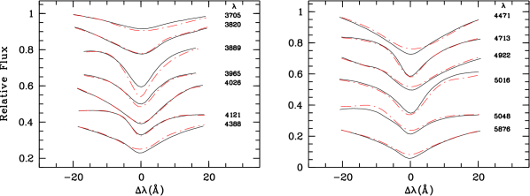
Figure 2: Strong lines in the average spectrum of GD 358 (full line) overlaid with a model (dot-dashed line) having $T_{\mathrm{eff}}$= 24 kK, $\log g=8$, and ML2/$\alpha=0.6$. Both the model and observed line profiles have been normalised in the same manner, with each line treated separately as described in Sect. 4.

Time-resolved spectra of GD 358 were obtained on 1999 June 23 using the Low Resolution Imaging Spectrometer (LRIS, Oke et al. 1995) mounted on the Keck II telescope. An 8$\aas@@fstack{\prime\prime}$7-wide slit was used together with a 600 line mm^-1 grating covering approximately 3500-6000 Å at 1.24 Å pixel^-1. The wavelength resolution was approximately 5 Å. A set of 612 20 s exposures were acquired from 06:53:12 to 12:37:55 U.T., bracketed by a series of arc and flatfield frames. The reduction of the data was carried out in the MIDAS environment and included the usual steps. Additionally, corrections for instrumental flexure and differential atmospheric refraction were applied. The procedure is nearly identical to that detailed in van Kerkwijk et al. (2000).

The seeing was $0\aas@@fstack{\prime\prime}$9 at the beginning of the run but deteriorated to 1$\aas@@fstack{\prime\prime}$5 towards the end of the run. This led to guiding problems which resulted in significant jitter (up to 2 pixels) of the target in the slit later in the run. We tried to correct for the jitter in the dispersion direction using the jitter in the spatial direction (which we could measure from the spatial profile), but found that the two were unfortunately uncorrelated. Not wanting to compromise the accuracy of our Doppler-shift measurements, we simply discarded the last 233 frames in the analysis that we describe below. Between 07:33:50 and 09:01:49 U.T. we found a constant offset in the pixel positions of the lines. We corrected for this shift using the mean offset as determined from frames taken before and after the above times. (see Fig. 3).

For flux calibration, 11 frames of the flux standard Wolf 1346 were taken, for which fluxes in 20 Å-wide bins were available. However, from previous observations, we have found that the response of the spectrograph shows small but significant variations over wavelength ranges smaller than 20 Å, and that these can be removed efficiently by using observations of stars for which well-calibrated model spectra are available. While these variations do not affect our analysis of the chromatic amplitudes (as these cancel out to first order), they do matter for the comparison of the mean spectrum with models. We therefore performed the flux calibration in two steps: we first calibrated all spectra with respect to the flux standard G 191-B2B (spectra for which were taken during a separate run but with an identical set-up) using the calibration of Bohlin et al. (1995), and then derived a (linear) response correction factor by comparing the observed spectrum of Wolf 1346 calibrated with respect to G 191-B2B with its own calibrated fluxes. This small correction factor was then applied to the time-averaged spectrum of GD 358 to ensure that the relative calibration would not affect the comparison with model spectra. We further scaled the mean spectrum (by a factor of 0.73) such that the estimated flux corresponded to the observed V-band magnitude.

4 Model atmospheres and the mean spectrum

Averaging together all spectra results in a high signal-to-noise mean spectrum that shows lines of He i only (Fig. 1).

By comparing with a grid of tabulated DB model atmospheres (details in Finley et al. 1997) spanning a range from 18-30 kK in steps of 500 K, and $\log g$ values from 7.5-8.5 in increments of 0.25 dex, we attempted to derive $T_{\mathrm{eff}}$ and $\log g$ from our mean spectrum. The model atmospheres consist of pure helium and were computed under the assumption of LTE; the description of line-broadening was taken from Beauchamp et al. (1997). Convective transport was taken to be of intermediate efficiency (ML2/$\alpha=0.6$). The parameter $\alpha$ denotes the mixing length as a fraction of the pressure scale height, with larger values of $\alpha$ corresponding to more efficient energy transport by convection. Several versions of the mixing length (ML) approximation abound. The original concept is due to Böhm-Vitense (1958). The ML2 version referred to above, with $\alpha=1$ is due to Böhm & Cassinelli (1971) and differs from the ML1 and ML3 prescriptions in the choice of certain parameters that determine the horizontal energy loss rate and thereby influence the convective efficiency.

Our best fit model with $T_{\mathrm{eff}}$$=24$ kK and $\log g=8.0$ is shown in Fig. 2. Each line was normalised separately, but in an identical manner for both the model and observed spectrum. The normalisation was carried out by dividing by the fit to the continuum points on either side of the line, thereby preserving the slope. We estimate the error in $T_{\mathrm{eff}}$ to be about 0.5 kK.

Small discrepancies between the model and the observations remain. These would normally be masked by a lower signal-to-noise spectrum. However, the results of Sect. 7 imply that these small discrepanices are probably real rather than being due to inadequacies in the flux calibration.

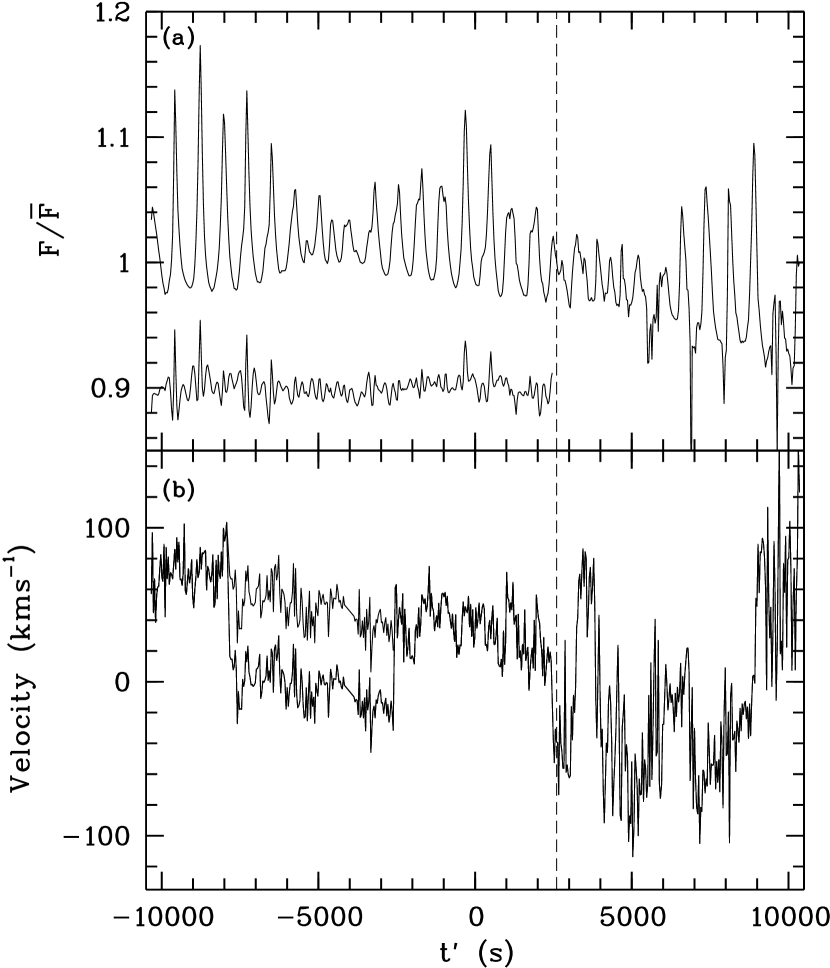
Figure 3: (a) Lightcurve of GD 358 showing a typical beat envelope. Note that the maxima are stronger and sharper than the minima. The lower curve shows the residuals (offset by +0.90) after fitting sinusoids with the amplitudes and phases listed in Table LABEL:gdtab. (b) The velocity curve as constucted by crosscorrelation. The vertical dashed line indicates the point ($t^{\prime}\gtrsim\ 2463$ s) beyond which the remainder of the frames were discarded. This was due to rapidly deteriorating seeing as discussed in Sect. 3. 8 additional frames from ($-4166\lesssim t^{\prime}(\mathrm{s})\lesssim-3899$) had to be deselected as these were markedly deviant from the expected mean position. The lower portion of the velocity curve between $-7410\lesssim t^{\prime}(\mathrm{s})\lesssim-2701$ shows the constant offset referred to in Sect. 3.

5 Light and velocity curves

5.1 Light curve

The lightcurve shown in Fig. 3a was constructed by dividing the line-free region of the spectra between $5100-5800$ Å by its average. The time axis was computed relative to the middle of the time-series ($t^{\prime}=t-9:35:33$ U.T.) in order to minimise the covariance between the amplitudes ($A$) and phases ($\phi$) of the sinusoids we use to fit the light curve. The Fourier Transform, calculated up to the Nyquist frequency, is shown in Fig. 4a. Periodicities were determined consecutively in order of decreasing amplitude by successively fitting functions of the form $A\cos(2\pi ft^{\prime}-\phi)+C$ where $f$ is the frequency, and $C$ a constant offset. The values we obtain for $f,A,$ and $\phi$ are listed in Table LABEL:gdtab. We first identified the real modes (i.e. those that were not obvious linear combinations) and then used these to fit the combination modes by fixing the frequency to the sum or difference of the real modes. We additionally imposed the requirement that the combination mode have an amplitude smaller than those of the two constituent real modes.

As is obvious from the residuals (Figs. 3a, 4a), the light curve is not free of periodicities after subtracting the frequencies listed in Table LABEL:gdtab. We have not attempted to look for lower amplitude modulations not only because our short time coverage and consequentially low frequency resolution means that the distinction between real and combination modes and noise peaks is blurred, but also because the determination of accurate periods and identifying all possible combination modes is not the principal aim of this investigation.

The frequencies that we measure for our real modes agree well with those measured for the two previous WET runs (Winget et al. 1994; Vuille et al. 2000) although detailed comparison is difficult, as the signal we measure is a blend of the various $m$ components. For instance, the peaks at 3886 $\mu$Hz ($\sim$3 F1) and 5182 $\mu$Hz ($\sim$4 F1) are probably due to combinations of unresolved multiplet components. We list our real modes together with the amplitudes, $n$, and $m$ determinations from the above studies in Table LABEL:tab:gdwet. The $m$-values listed are the closest match between our periods and frequencies compared to those listed in Table 3 of Vuille et al. (2000) only.

Figure 4: (a) Fourier Transform of the light curve and residuals offset by $-0.6$% and (b) of the velocity curve shown up to 8500 $\mu$Hz with the residuals offset by $-2.7$ $\rm km\,s^{-1}$Ṫhe strongest peaks in the FT of the light curve are labelled. There are no peaks greater than $\sim$ 0.08% and $\sim$2.7 $\rm km\,s^{-1}$ longward of 8500 $\mu$Hz.

Table 2: Pulsation frequencies and other derived quantities from the light and velocity curves of GD 358.

Mode	Period	Frequency	$A_{L}$	$\Phi_{L}$	$A_{V}$	$\Phi_{V}$	$R_{V}$	$\Delta\Phi_{V}$
	(s)	($\mu$ Hz)	(%)	(°)	($\rm km\,s^{-1}$)	(°)	(Mm rad${}^{-1})$	$(\degr)$
Real Modes:
F1 (17)	776.42 $\pm$ 0.54	1288.0 $\pm$ 2.6	3.10 $\pm$ 0.18	$-$128 $\pm$ 03	4.6 $\pm$ 1.1	$-$126 $\pm$ 14	18 $\pm$ 04	$-$02 $\pm$ 14
F2 (15)	702.39 $\pm$ 0.75	1423.7 $\pm$ 1.5	2.29 $\pm$ 0.08	$-$153 $\pm$ 03	5.6 $\pm$ 1.0	0$-$95 $\pm$ 10	27 $\pm$ 05	$-$59 $\pm$ 11
F3 (18)	809.28 $\pm$ 0.29	1235.7 $\pm$ 6.5	1.07 $\pm$ 0.17	$-$071 $\pm$ 09	4.0 $\pm$ 1.1	$-$077 $\pm$ 16	48 $\pm$ 14	$-$05 $\pm$ 18
F4 (9)	464.44 $\pm$ 0.10	2153.1 $\pm$ 5.1	0.66 $\pm$ 0.08	$-$089 $\pm$ 10	3.3 $\pm$ 1.0	$-$150 $\pm$ 17	37 $\pm$ 11	$-$61 $\pm$ 20
F5 (8)	424.26 $\pm$ 0.78	2357.1 $\pm$ 4.3	0.62 $\pm$ 0.08	$-$116 $\pm$ 10	1.9 $\pm$ 1.0	$-$164 $\pm$ 29	21 $\pm$ 11	$-$81 $\pm$ 31
Combinations:
Mode	Period	Frequency	$A_{L}$	$\Phi_{L}$	$A_{V}$	$\Phi_{V}$	$R_{C}$	$\Delta\Phi_{C}$
	(s)	($\mu$ Hz)	(%)	(°)	($\rm km\,s^{-1}$)	(°)		$(\degr)$
2F1	388.21	2575.9	1.12 $\pm$ 0.11	$-$105 $\pm$ 08	2.5 $\pm$ 1.1	$-$$\cdots$	12 $\pm$ 2	$-$01 $\pm$ 10
F1+F2	368.78	2711.7	0.55 $\pm$ 0.11	$-$083 $\pm$ 11	0.8 $\pm$ 1.2	$-$$\cdots$	04 $\pm$ 1	$-$05 $\pm$ 11
F2+F5	264.50	3780.8	0.52 $\pm$ 0.08	0$-$91 $\pm$ 10	1.8 $\pm$ 1.0	$-$$\cdots$	18 $\pm$ 4	$-$53 $\pm$ 14
F2+F3	376.03	2659.4	0.48 $\pm$ 0.09	$-$101 $\pm$ 14	1.0 $\pm$ 1.1	$-$$\cdots$	10 $\pm$ 2	$-$19 $\pm$ 17
F1+F3	396.26	2523.6	0.48 $\pm$ 0.13	0$-$40 $\pm$ 15	0.8 $\pm$ 1.1	$-$$\cdots$	07 $\pm$ 2	$-$17 $\pm$ 18
2F2	351.20	2847.4	0.31 $\pm$ 0.08	$-$032 $\pm$ 15	1.2 $\pm$ 1.0	$-$$\cdots$	06 $\pm$ 2	$-$22 $\pm$ 16

Notes. The number in brackets next to the mode name indicates the $n$ value from previous WET studies, based on their $\ell=1$ identification for all modes. The velocity to flux amplitude ratio $R_{V}=A_{V}/(2\pi fA_{L})$, and phase $\Delta\Phi_{V}=\Phi_{V}-\Phi_{L}.$ The photometric amplitude for combination modes with respect to the real modes that make up the combination is given by $R_{C}=A_{L}^{i\pm j}/(n_{ij}A_{L}^{i}A_{L}^{j})$ where $n_{ij}=2$ for 2-mode combinations involving two different modes, and 1 for the first harmonic of a mode; the relative phase of combination modes is defined as $\Delta\Phi_{C}=\Phi_{L}^{i\pm j}-(\Phi_{L}^{i}\pm\Phi_{L}^{j})$.

5.2 Velocity curve and significance of detections

In order to search for any variations in the line-of-sight velocity we cross-correlated our 379 usable spectra using the mean spectrum as a template. Having thus constructed a velocity curve (Fig. 3b) we attempted to fit it in exactly the same way as described above, except that we fixed the frequencies to those derived from the light curve (Table LABEL:gdtab) leaving the amplitudes and phases free to vary. A low-order polynomial was included in the fit in order to remove any slow variations. Given the presence of noise especially at the low frequency end, this imposition of frequencies from the light curve is a use of additional independent information, and merely reflects our (reasonable) assumption that we expect the same frequencies to be present in the velocity curve as those found in the light curve.

As our spectra were taken through a wide slit (to preserve photometric quality), the positions of the spectral lines depend on the exact position of GD 358 in the slit. Although this position should be tagged to the position of the guide star, we found that additional random jitter (e.g. due to guiding errors, windshake) was present. An estimate of the scatter in the measured velocities due to wander can be obtained from shifts in the slit of the spatial profile under the assumption that these shifts are also representative of the scatter in the dispersion direction. We fitted Gaussians to the spatial profiles and took the standard deviation of the centroid positions as a proxy for the scatter; we find a value of 9 $\rm km\,s^{-1}$ at a representative wavelength of 4471 Å. Including this value in the least squares fit of the velocity curve results in a $\chi_{\mathrm{red}}^{2}\simeq 1$. The velocity amplitudes and phases we find are listed in Table LABEL:gdtab.

As a cross-check, we fitted 13 of the strongest lines (marked in Fig. 1) in all 379 spectra with a combination of a Gaussian and a line or a 2^nd-order polynomial to represent the continuum and constructed an average velocity curve using the Doppler shifts of all 13 lines. Typical uncertainties in the fitting of the line profiles are of the order of 14 $\rm km\,s^{-1}$ at $\lambda$4471 Å. We then fit this velocity curve in exactly the same manner as described above and found good agreement (within the quoted errors) with both the velocity amplitudes and phases derived from the cross-correlation procedure.

For the DAVs, the derivation of the velocity curve using the cross-correlation technique is not reliable (see the discussion in van Kerkwijk et al. 2000) due to changes in the continuum slope during the pulsations – an effect that is not taken into account in the cross-correlation procedure. The higher effective temperatures of the DBVs however, means that the continuum slope is not severely affected and therefore does not bias the Doppler shifts, making the procedure more reliable.

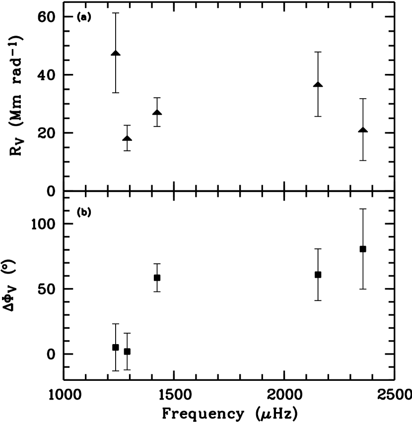
Figure 5: (a) The relative velocity to light amplitude $R_{V}=A_{V}/2\pi fA_{L}$ and (b) $\Delta\Phi_{V}$, the phase difference between velocity and light, for the 5 real modes.

In order to obtain quantitative estimates of the significance of our measured velocity amplitudes and to ascertain the contribution of random noise peaks, we conducted a simple Monte Carlo test: we randomly shuffled the velocities with respect to the observation times and fit the resulting velocity curve in exactly the same way as the observations (as described above). We repeated the procedure 1000 times and counted the number of times a peak larger than that observed was found exactly at the frequency of each of the real modes. We found that the peak at F2 had a $\la 0.1$% chance of being a random peak while those at F1, F3, and F4 had a likelihood of 2%, 5%, and 9% respectively of being chance occurrences. All other peaks were found to be insignificant. We conclude therefore, that the modulations we see in the Doppler shifts are due to intrinsic processes and that these are line-of-sight velocity variations associated with the pulsations. In what follows, we include all real modes and treat the velocity amplitudes of those that were only marginally significant as upper limits.

We note as an aside that Provencal et al. (2000) invoke the velocites associated with the oscillatory motions to explain the width ($v\sin i\sim 60$ $\rm km\,s^{-1}$) of the C ii $\lambda$ 1335 Å line. Our measured velocities do not support this speculation. The interpretation of the broad and shallow profiles as being due to a high rotational velocity is also at odds with that inferred from the rotationally-induced splittings (0.9 days for the core to 1.6 days for the envelope, Winget et al. 1994). Interestingly, several slowly rotating DAVs too show broad and flat (H$\alpha$) line cores, although this observation is not unique to the pulstors (Koester et al. 1998).

Table 3: Comparison with the WET data sets

	Period	$n$	$m$	WET 90	WET 94	Keck 99
				Amplitude
	(s)			(%)	(%)	(%)
F1	776.42	17	$-$1,(0)	0.49 (1.45∗)	0.64 (2.21∗)	3.10
F2	702.39	15	$-$0	1.9∗	1.66	2.29
F3	809.28	18	$-$0	$\sim 0.3^{*}$	1.36∗	1.07
F4	464.44	9	$-$0,1	0.45∗,0.27	0.48∗,0.27	0.66
F5	424.26	8	$-$1,0	0.49,0.5∗	0.45,0.92∗	0.62

Notes. The WET 90 and WET 94 results are from Winget et al. (1994) and Vuille et al. (2000). respectively; all modes listed here were identifed in these studies as having $\ell=1$. Note that small (0.03 - 2 $\mu$Hz) frequency shifts – of unknown origin – were found between the two WET data sets. The $n$ and $m$ values listed here are simply chosen from Vuille et al. (2000) that are closest to our measured values. As the frequency splitting decreases with decreasing $n$, the difficulty in discriminating between the various multiplet components within a triplet observed in the WET data and our single mode, increases. An asterisk next to the mode amplitude indicates that this mode had the largest amplitude in the triplet. We remind the reader that our amplitudes are a blend of the different $m$ components. For the $n=17$ triplet, we indicate the $m$ component that had the largest amplitude in both WET datasets in brackets for comparison purposes. Note that for some reason, Winget et al. (1994) do not list the amplitude for the $n=18$ mode in their Table 2 even though it is clearly present and shows many combinations. The value above has been obtained by reading off the value from their Fig. 3.

6 Real modes

Following van Kerkwijk et al. (2000), we adopt $R_{V}=A_{V}/2\pi fA_{L}$ and $\Delta\Phi_{V}=\Phi_{V}-\Phi_{L}$ as measures of the relative velocity to flux amplitude ratio and phase difference, respectively, for the real modes. We list these values in Table LABEL:gdtab, and plot them as a function of mode frequency in Fig. 5.

As a (real) mode propagates upward, its environment changes from being largely adiabatic (velocity maximum lags flux maximum by 90°), to one where non-adiabatic effects are important. If $R_{V}$ and $\Delta\Phi_{V}$ follow the expected trends, they can be used to constrain the properties of the outer layers of the white dwarf. We describe these trends below.

In the convection zone, flux attenuation increases with increasing mode frequency i.e., $A_{L}$ decreases. However, turbulent viscosity in the convection zone ensures negligible vertical velocity gradients, with the result that the horizontal velocities are effectively independent of depth within the convection zone (Brickhill 1990; Goldreich & Wu 1999b). Thus, the ratio between the velocity and flux amplitudes ($R_{V}$) is expected to increase with increasing mode frequency. Fig. 5a shows no such trend.

For the adiabatic case, the phase lag between velocity and light is expected to be 90$\degr$; non-adiabatic effects reduce this lag. $\Delta\Phi_{V}$ is therefore expected to lie between 0$\degr$ and 90$\degr$. This is indeed found to be the case (Table LABEL:gdtab). As higher frequency modes are increasingly delayed by the convection zone, $\Delta\Phi_{V}$ should tend to zero with increasing mode frequency. Although the error bars are large, Fig. 5b shows a trend opposite to the one just described. It is worth noting that van Kerkwijk et al. (2000) also found some indication of such a trend in their analysis of ZZ Psc (a DAV type pulsator).

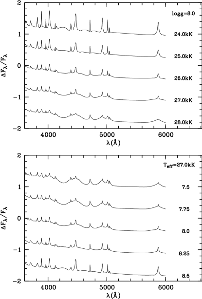
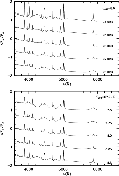
Figure 6: Top panel: Model chromatic amplitudes (using ML2/$\alpha=0.6$) for $\ell=1$ showing the effect of varying the effective temperature at constant $\log g$ within the wavelength range of our observations. Bottom panel: Same as above, but for varying $\log g$ at constant effective temperature. The offset between the models is 0.7. All models have been convolved with a Gaussian having a FWHM of 4.1 Å to emulate a seeing profile. The panels on the left are for $\ell=1$ while those on the right are for $\ell=2$.

Apart from the effect of increasing delay, another effect, that of increasing non-adiabaticity with mode period (Goldreich & Wu 1999b), might also be at play. Indeed, Fig. 5b shows that the relative phase between velocity and flux decreases as a function of mode period. It is difficult to estimate the relative importance the two effects. Perhaps also of relevance to the above is the discontinous change in horizontal velocity across the boundary between the radiative interior and the convective layers (Goldreich & Wu 1999b). The shear layer at this boundary might be expected to impart not insignificant phase shifts to the horizontal velocities since the spatial acceleration due to viscous forces is roughly an order of magnitude larger than the pressure perturbation for DAVs (see Fig. 11 in Gautschy et al. 1996). Whether this is indeed the case would have to be checked by investigating the behaviour of the modes in the presence of such a shear layer. It is not immediately evident from the description of Goldreich & Wu (1999b) how the phases of the horizontal velocities are affected across this jump as a function of mode period.

Figure 7: Observed chromatic amplitudes, calculated in 3 Å wide bins, shown here for the 5 real modes and the strongest combination mode. The periods are indicated next to the names.

Figure 8: Same as Fig. 7, but showing the effect of removing the average Doppler shift on the chromatic amplitudes for F1 – F5. The effect is most clearly seen e.g. in the $\lambda$4713 Å line of F3. Note the lack of significant change (c.f. Fig. 7) for 2F1.

7 Chromatic amplitudes ($\mathbf{\Delta F_{\lambda}/F_{\lambda}}$)

As mentioned in Sect. 1, the fractional pulsation amplitudes calculated as a function of wavelength bear an $\ell$-dependent signature. Even though all non-radial modes suffer from cancellation which occurs as a result of observing disc-integrated light, the cancellation increases with increasing $\ell$. As limb-darkening increases at shorter wavelengths, the effect of this cancellation is reduced, resulting in a net increase of pulsation amplitudes (for $\ell\leq 3$). A similar effect is also apparent at optical wavelengths, especially in the absorption lines. Comparing fractional amplitudes has the added advantage that uncertainties in the data acquisition and reduction processes are expected to cancel out; any differences between the synthetic and observed chromatic amplitudes are therefore intrinsic.

The model atmospheres described in Sect. 4 have intensities tabulated at nine different limb angles. We used these to compute a grid of synthetic chromatic amplitudes by integrating over these intensities, weighted by Legendre polynomials which describe the surface distribution of the temperature perturbations. The change in intensity with respect to temperature (as a function of the limb angle) was computed using adjacent models of different effective temperature.

The effect of varying the effective temperature and $\log g$ is shown in Fig. 6. Contrary to the case of the DA pulsators (Clemens et al. 2000), the models display a remarkable sensitivity to small changes in these model parameters. If the models are able to match the observations, this sensitivity could be exploited to provide a new way of measuring $T_{\mathrm{eff}}$ and $\log g$. The differences between $\ell=1$ and $\ell=2$ in the models are similar to the DA case, in that the continuum between the lines is more curved and the line cores sharper for the latter case.

To compare with models, we constructed a 2-D (wavelength-time) stacked image from our spectra and calculated the fractional pulsation amplitudes as a function of wavelength by fitting for the amplitudes and phases of the modes listed in Table LABEL:gdtab, the frequencies being held fixed to the tabulated values. The resulting chromatic amplitudes and phases for all real modes are shown in Figs. 7 and 9.

Figure 9: Observed chromatic phases shown here for all real modes and the strongest combination mode.

Clemens et al. (2000) were able to assign $\ell$ values to the real modes in ZZ Psc by comparing the observed chromatic amplitudes with each other. As they showed, simple inspection of the chromatic amplitudes, especially when modes with different $\ell$ values are present, works well. This is particularly true when the target is bright. Before comparing the chromatic amplitudes of GD 358 with the models, we note that all the real modes have the same general shape to one another implying that they share the same $\ell$ value (especially F1 and F2 which are nearly identical); given the WET results, this is most likely $\ell=1$.

The only exception to the above is F3 (Fig. 7) which exhibits some differences compared to the other modes, most notably in the shape and strength of the line cores at $\lambda$4120, 4713, and 5047 Å. The first and last of these three lines are barely discernible in the chromatic amplitudes of the other four real modes. Although the amplitudes of the line cores are in general greater for $\ell=2$ than $\ell=1$ modes, it is difficult to disentangle the effect of a different spherical degree from the dependence on the effective temperature and $\log g$. We also note that F3 has the highest velocity to flux amplitude ratio ($R_{V}$). Even though the differences are admittedly not significant compared to the other modes, a higher $R_{V}$ can be indicative of a higher $\ell$ value as the light variations for such modes suffer greater cancellation than the horizontal velocity variations (Dziembowski 1977).

While the difference in appearance is significant, one has to be careful in assigning a cause. In principle, line-of-sight variations that are in phase with the light curve, could induce differences in relative amplitude as well (see Clemens et al. 2000). These scale with $dF_{\lambda}/d\lambda$ and thus should be most pronounced near sharp lines. This is indeed seen for F3, which additionally has the highest value of $R_{V}\cos\Delta\Phi_{V}$, i.e., for F3 the line-of-sight velocity variations are expected to have the largest effect on the chromatic amplitudes. In order to test whether this was indeed the underlying cause of the difference in appearance, we removed the Doppler shift from all the spectra (using the average velocities shown in Fig. 3) and recomputed the chromatic amplitudes. The result is shown in Fig. 8. Clearly, having taken out the effect induced by the line-of-sight velocity variations, F3 becomes very similar in appearance to F1 and F2. On the basis of this, we conclude that F3 too shows $\ell=1$-like behaviour. This is consistent the WET 1994 data which shows a triplet at this period, indicative of an $\ell=1$ mode. We stress, though, that the above leaves open the question of why F3 has a larger $R_{V}\cos\Delta\Phi_{V}$.

It is interesting to note that the chromatic amplitude of the strongest combination mode, 2F1, is different in appearance compared to the five real modes, in that it has a larger curvature in the continuum between the lines cores (Fig. 7). This is probably due to a dominant $\ell=2$ component (see Fig. 6).

Incidentally, this is to be expected if our match – based on Vuille et al. (2000) – of $m=-1$ is correct (Table LABEL:tab:gdwet), since a combination of $Y_{1}^{-1}Y_{1}^{-1}$ (where the $Y_{\ell}^{m}$ are spherical harmonics) has a distribution described by $Y_{2}^{-2}$ only. We cannot, however, definitively rule out the possibility that F1 has $m=0$ or $m=1$ which would mean the presence of a $Y_{0}^{0}$ component in the former case in addition to the $Y_{2}^{0}$ component. Unfortunately, the weakness of the other combinations means that we cannot subject them to a meaningful test.

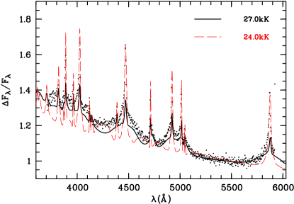
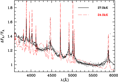
Figure 10: Left: The observed chromatic amplitude for the mode having the largest amplitude flux variations, F1, (dots) overlaid with models calculated at the two different effective temperatures with $\log g=8$ for $\ell=1$ modes and with intermediate convective efficiency. Right: For models having $\ell=2$

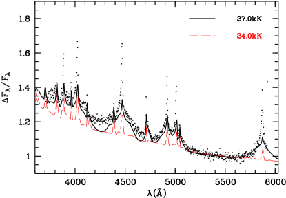
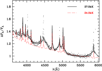
Figure 11: Left: Same as for Fig. 10, but with the models calculated using a lower convective efficiency (ML1/$\alpha=0.5$). For $\ell=1$. Right: For $\ell=2$.

Although our fit to the mean spectrum (Fig. 2) is arguably reasonable, we find that for the effective temperature derived from the spectrum (24 kK), the model chromatic amplitudes do not even look qualitatively similar to the observations. Fig. 10 shows the chromatic amplitude of the strongest mode (F1) compared to synthetic chromatic amplitudes for two effective temperatures each for $\ell=1$ and $\ell=2$. We can only match the shape of the pseudo-continuum between the line cores if we use models with higher ($\sim$ 27 kK) temperatures.

We do not expect to fit the line cores as these are probably formed in parts of the atmosphere where $\tau\ll 1$ and where, as a result, deviations from LTE might be important. The (pseudo-)continuum, however, should not be affected and we stress that it is these regions of the chromatic amplitudes that we seek to match.

We see that the observed wings of the lines are broader than those of the models calculated using an intermediate convective efficiency (ML2/$\alpha=0.6$). Less efficient convection would make the temperature gradient steeper. To test whether the temperature stratification of the models is the culprit, we calculated models in which the convective efficiency was three times lower. In Figs. 10 and 11 we compare models having different convective efficiencies to the data and see that there is a slight improvement to the match in the wings of the lines for the model having a lower convective efficiency (ML1/$\alpha=0.5$) but that the match in some of the continuum regions has worsened. It may be possible to reproduce the chromatic amplitudes with a different choice of mixing length or mixing-length prescription. However, we feel this is unlikely, as we failed to reproduce the chromatic amplitudes for ZZ Psc even with a very extensive set of models. We will return to this briefly below.

Phase changes within the lines due to the line-of-sight velocity variations are apparent (Fig. 9) especially for the stronger lines. As in previous studies of this nature of DA pulsators, we find a very slight ($\sim$1°) slope in phases over the wavelength range although this is much less obvious than was found for at least two DAVs (van Kerkwijk et al. 2000; Kotak et al. 2002a).

8 Discussion and conclusions

As outlined at the outset, our main aims were to investigate the pulsation properties of GD 358, to compare these with the better studied DAVs, and to use our data to place constraints on model atmospheres.

We began by determining the modulations present in the light curve and found that all five real modes agreed very well with previous WET observations.

We also found variations in the Doppler shifts of the spectral lines that were coincident with those determined from the light curve. We concluded that these were line-of-sight velocity variations associated with the largely horizontal motion of the pulsations.

Using the velocity to light amplitude ratios ($R_{V}$) and phases ($\Delta\Phi_{V}$) we tested theoretically expected trends. We found no evidence for a general increase in $R_{V}$ with mode frequency. This has also been the case for the DAVs. Although $\Delta\Phi_{V}$ was found to lie between 0 and 90°, as expected we found some evidence that it increases with mode frequency – a trend opposite to that predicted. Previous measurements of the DAVs (van Kerkwijk et al. 2000) have also found marginal evidence for such a trend.

The wavelength-dependent fractional pulsation amplitudes proved to be invaluable in two altogether different ways. First, the resemblance of most of the observed chromatic amplitudes to each other led to the conclusion that they all shared the same spherical degree, most likely, $\ell=1$. Our results provide an entirely independent confirmation of the WET results.

We also showed that the chromatic amplitude of 2F1 was different, and bore the signature of an $\ell=2$ mode. Our $m$ identification – based on the WET 1994 results – suggests that F1 has $m=-1$. If true, it implies a redistribution of power between the $m$ components in that triplet, which previously showed a dominant $m=0$ component (see Table LABEL:tab:gdwet).

Secondly, although our synthetic chromatic amplitudes failed to reproduce the observations for any combination of $T_{\mathrm{eff}}$ and $\log g$, they unambiguously indicated that a temperature higher than that inferred from our mean spectrum ($T_{\mathrm{eff}}$=24 kK; $\log g$=8) was a better match at all wavelengths. Thus while our average spectrum favours a lower temperature, the chromatic amplitudes indicate a higher temperature, in agreement with temperature determinations based on ultra-violet spectra. The cause of this discrepancy remains unexplained.

We also found that the chromatic amplitudes could be reproduced only qualitatively, with the models failing to reproduce both the cores and the wings of the lines. Slight improvement is obtained – mainly in the wings of the lines – with models of lower convective efficiency than ML2/$\alpha=0.6$. In detail, however, the models still do not match, as is also the case for the DAV ZZ Psc (Clemens et al. 2000) even when trying models for a much more extensive set of mixing-length parameters. The above may mean mean that there is an intrinsic problem with the atmospheric models, e.g., that the real temperature structure simply cannot be reproduced accurately enough with the mixing-length approximation. If so, perhaps the observations can be used to derive the temperature stratification empirically.

Alternatively, there may be a problem with the way that the atmospheric models are used to calculate model chromatic amplitudes. In particular, our calculations assume that the temperature variations associated with the pulsations are described well by a single spherical harmonic, and we take into account only the first derivative of the flux with respect to temperature. The latter effect is rather small, but the former may be important: Ising & Koester (2001) used numerical simulations to investigate these issues and found that as the amplitude of a mode increases, the surface flux distributions do deviate more and more from spherical harmonics. The effects become pronounced for pressure perturbations larger than about 10%, which correspond to visual flux variations with amplitudes of about 5% for DAV and 3% for DBV, i.e., at about the level observed for the strongest modes.

No direct comparison of these models with observations has yet been made, but an empirical estimate can be made by considering all the non-linearities in terms of combination frequencies. Clearly, second-order corrections cannot influence the chromatic amplitudes of a real mode, since these corrections appear as harmonics, sums, and differences of the real modes. Third-order corrections, however, will have terms – such as 2F1${}-{}$F1 and F1+F2$-$F2 – which coincide with the real modes, but are described by surface distributions with different $\ell$ and can thus influence the shape of the chromatic amplitudes measured at the frequency of the real mode. Indeed, Vuille et al. (2000) find a large number of third-order combination frequencies for GD 358, with amplitudes up to a quarter of those of the real modes. While this is a significant fraction, one should bear in mind that their surface flux distribution will be dominated by their $\ell=0$, 1, and 2 components, which will not change the inferred chromatic amplitudes much. It thus remains unclear whether or not these higher-order terms can be responsible for the mismatch between the observed and model chromatic amplitudes.

Fortunately, there is a clear prediction: for low-amplitude pulsators, which show no or only very weak combination modes, the chromatic amplitudes should not be influenced by higher-order corrections. Thus, if the chromatic amplitudes of such pulsators can be matched by models, higher-order corrections are at play for the mismatches observed so far. If they do not, the problem must be one intrinsic to the model atmospheres. With accurate observations of low amplitude DBVs and detailed models, we can expect rapid progress.