Density gradients and internal dust in the Orion nebula

Abstract

The ionization structure of the Orion nebula can be described as a skin-like ionization structure on the surface of a dense cloud. We propose that a steep density stratification, increasing as a powerlaw ($n\propto x^{-2}$) function of distance $x$ from the ionization front, exhibits properties which agree with our long-slit spectrum of the Orion nebula. For instance, there exist a unicity relation between both the H$\beta$ surface brightness or the ionization front [S ii] density, and the scale $L$ of the powerlaw, where $L$ is the distance between the ionization front and the onset of the density near the exciting star. Internal dust is required to obtain a simultaneous acceptable fit of both the [S ii] density and then H$\beta$ suface brightness observations. Nebular models containing small dust grains provide a better fit than large grains. The line ratio gradients observed along the slit are qualitatively reproduced by our density stratified models assuming a stellar temperature of 38000 K. Collisional deexcitation appears to be responsible for half of the gradient observed in the [N ii]$\lambda$5755/[N ii]$\lambda$6583 temperature sensitive ratio. We propose that the empirical relationship found by Wen & O’dell between density and stellar distance may possibly be caused by a power-law density stratification.

0.1 Introduction

It was recognized early on by Münch (1958) and Wurm (1961) that the Orion nebula is better described as a photoionized skin on the surface of a dense cloud than by a uniformly filled gas structure. Furthermore, kinematics of the ionized gas (see review by O’Dell 1994) indicates the gas is flowing away from the dense ionizing front on the surface of the molecular cloud. Although earlier studies proposed an exponential function to describe the density behaviour from such a flow (Tenorio-Tagle 1979; Yorke 1986), more recent theoretical and observational works (Franco, Tenorio-Tagle & Bodenheimer 1989, 1990; Franco et al 2000a,b) indicate that expanding H ii regions are well described by a power law density stratification $n\propto x^{-\beta}$ with exponents larger than $\beta=1.5$. This is qualitatively consistent with the results obtained from hydrodynamic calculations of photoevaporative flows off proplyd disks by Richling & Yorke (2000) or off spherical surfaces by Bertoldi (1989) and Bertoldi & Draine (1996). The current paper looks at how the observed gradient of the [S ii] density in Orion can be accounted for using a simple powerlaw density model and how well the surface brightness compares with the long-slit observations presented here. The aim is to explore the benefits of a powerlaw density stratification in the context of a determination of the shape of the ionization front (hereafter IF) using a surface brightness map in H$\alpha$, a task first performed by Wen & O’Dell (1995) for the two cases of isochoric and exponential density behaviour.

0.2 Observations and data reduction

We have taken long-slit spectra of the central region of Orion at the Observatorio Astrofísico Guillermo Haro, Cananea, on the 21st of December 1998 using a $1024\times 1024$ TEK CCD detector mounted on a Boller & Chivens spectrograph. We used a grating of 300 l/mm and covered the wavelength range 3600–5200 Å, 5500–7100 Å, and 8000–9600 Å in three settings. The corresponding exposure times were 90, 60 and 300 seconds, respectively. A slit width of 2.5 was used. The effective spectral resolution was $\approx 6$ Å. The slit was aligned West-East and off-centered by 30 to the South of $\theta^{1}$ C Ori as illustrated in Fig. 1. Arc spectra were taken as well as standard star exposures. Data reduction (bias subtraction, flat fielding, wavelength and flux calibration) was performed with IRAF. Due to non-photometric conditions and partial cloud coverage, we could not derive a reliable absolute flux calibration. We hence used the calibration of Rodríguez (1999), who had also observed with the slit aligned East-West with her regions A-1 and A-3 common to ours. We tied our H$\beta$ fluxes to the mean surface brightness within her region A-1. In any event, the adopted Rodríguez surface brightness value is only 25% higher than our initial calibration. Line fluxes were reddening corrected using the Balmer decrement and the galactic reddening law (Seaton 1979). Further details on the data can be found in González-Gómez (1999).

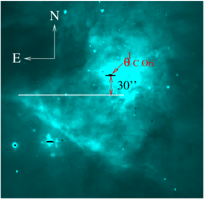
Figure 1: Image illustrating the position of our long-slit on an R-band image of Orion. The position of the exciting star $\theta^{1}$ C Ori (whose image is saturated) is indicated. The R-band filter encompasses H$\alpha$ and the red [N ii] lines which account for most of the nebular emission visible on the image.

0.3 The photoionization models

We adopt a similar approach to that of Binette & Raga (1990, hereafter BR90) who studied the properties of powerlaw densities in photoionized slabs (see also Williams 1992). However, we adapted their simple slab geometry to the more appropriate spherical geometry for reasons given below in Sect.0.3.2. Another paper which considers powerlaw density stratification in photoionization models is that of Sankrit & Hester (2000) (see also Hester et al. 1996).

The emission line measures in Orion are dominated by the gas near the IF as a result of the strong density gradient towards it. In the work of Wen & O’Dell (1995, hereafter WO95), the authors approximated the front structure as gas segments (or columns) aligned towards our line of sight with a projected area on the sky of $2\arcsec\times 2$. In their final best model, the densities within the segments declined exponentially towards the observer rather than radially towards $\theta^{1}$ C Ori. Using the observed distribution of H$\alpha$ surface brightness and [S ii] gas density, WO95 were able to solve for the IF distance (along our line of sight) for the whole nebula. Such a distribution of distances is termed the “shape” of the IF. The gas segments of their model did not extend up to the exciting star, a characteristic also shared by the isobaric slab model of Baldwin et al. (1991, hereafter BF91). In such a scheme, the segments are independent and a density must be specified for each segment. In this Paper, we will explore density distributions which are exclusively function of radius from $\theta^{1}$ C Ori without assuming any significant gas cavity near $\theta^{1}$ C Ori.

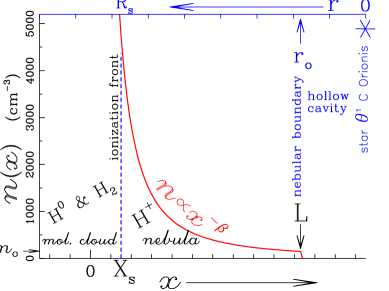
Figure 2: Diagram illustrating qualitatively our powerlaw density stratification as a function of $x$. The origin of the spatial $x$ axis lies at a depth $L$ from the nebular boundary and the density at that position (at $x=L$) is labelled $n_{o}$ (see Equation 1). Note that $L$ will be allowed to vary with angular direction from $\theta^{1}$ C Ori. The top axis is the radial distance $r$ from the star $\theta^{1}$ C Ori, with $r$ increasing towards the left. The IF (or inner Strömgren boundary) is situated at $X_{s}$ (or equivalently at $R_{s}$). The electronic density inferred from the [S ii] doublet corresponds to a density near the IF. The hollow gas cavity surrounding the star has a size $r_{o}$. In our models, the adopted value for $r_{o}$ is much smaller than depicted above.

0.3.1 The radial density gradient

We adopt a similar notation to BR90 in which the density profile (with an origin lying inside the dense cloud) is described as follows:

$$\begin{array}[]{lr}n(x)=n_{o}\left({L\over x}\right)^{\beta}\;;x\leq L\,,\\ n(x)=0\;\;x>L\,,\end{array}$$ (1)

where $n(x)$ is the gas density, $\beta$ the powerlaw index ($n\propto x^{-\beta}$), $n_{o}$ the boundary density of the nebula towards the exciting star, and $x$ the variable representing the distance from the inner density discontinuity at $x=0$. Note the reversal of axis relative to traditional studies: the ionizing radiation is entering at the cloud boundary $x=L$ and is absorbed inward up to the inner Strömgren boundary at $X_{s}$ (see Fig. 2). The steep density gradient near the origin ensures that the photons are absorbed before the density discontinuity, hence $X_{s}\ga 0$.

In the case of Orion, the spherical geometry is necessary in order to take into account the geometrical dilution of the ionizing radiation across the radial density structure. One can define the variable, $r$, as the distance from the central ionizing star; that is $r=L-x+r_{o}$ where $r_{o}$ is the radius of the central hollow cavity and $n_{o}$ the gas density at $r_{o}$. When the ionizing photon luminosity $Q_{H}$ is sufficiently high (or the density $n_{o}$ low), the Strömgren radius, $R_{s}=L-X_{s}+r_{o}$, is near the origin of the $x$ axis, at a distance $\simeq L+r_{o}$ from the exciting star (since $X_{s}$ is negligible). This is referred by BR90 as the “strong gradient” regime. In the converse case, for very low ionizing photon luminosities $Q_{H}$ (or for high boundary densities $n_{o}$), $R_{s}$ shrinks ($X_{s}$ becomes non-negligible) and becomes of order $r_{o}+$ small fraction of $L$, a condition which BR90 labeled “weak gradient” because the nebula’s thickness is smaller than the density gradient’s scale $L$. All the quantities introduced above are illustrated in Fig. 2.

The “strong gradient” regime is the appropriate one for Orion since the nebula is traditionally approximated by a skin-like structure on the face of a dense molecular cloud (BR90; O’Dell 1994). One advantage of the powerlaw stratification when the regime of “strong gradient” prevails is that we know before hand the approximate radius of the IF ($\la L+r_{o}$). In the case of an exponential stratification, which is much shallower than a powerlaw, it requires solving for the ionizing radiation transfer inside the nebula in order to predict the IF depth.

For definiteness, we will consider the case of a powerlaw index $\beta=2$. Very similar nebular line ratios of [O ii], [O iii], etc. were obtained with indices of $\beta=1.5$ and 1.0, provided we adjusted $n_{o}$ and $L$ in such a way that both the ionized depth $R_{s}$ and the [S ii] density remained the same as that obtained with the $\beta=2$ case. We consider that our results do not depend on the particular choice of $\beta$ made here.

We found no justification for having an arbitrary large region devoid of gas around $\theta^{1}$ C Ori and, for definiteness, have set $r_{o}=0.007{\rm pc}\la 0.05R_{s}$, a size so small that its precise value has no impact on the calculations.

0.3.2 The geometry

The geometry of the IF is highly structured and complex (c.f. WO95) and cannot be modeled directly by a code like mappings ic which is designed to handle simple nebular geometries. Our approach has been to compute a sequence of spherical models of different scale $L$ (c.f. Equation 1) in order to simulate small areas of the IF located at different distances from the exciting star. This piecemeal approach (a different model for each position along the slit) allowed us to reconstruct the IF contribution through each aperture element. To account for the projection of each slit aperture element onto the calculated Strömgren spheres, we carried out in mappings ic the integral of line emissivities over spatial limits corresponding to the appropriate aperture projection onto the calculated spheres.

Our aim is to model only the background IF (the component B in BF91) which is much brighter than the foreground IF (the component A in BF91). We therefore halved the fluxes computed by mappings ic to reduce the geometry to that of an hemisphere rather than a sphere. Furthermore, to remove the small contribution due to component A, we multiplied the observed H$\beta$ surface brightness by $\case{4}{5}$, the same value as in BF91.

To sum up, the different IF positions covered by the slit are associated to a sequence of models which differ only by their value of the scale $L$. Since our slit was offset to the South by 30 from $\theta^{1}$ C Ori (extending mostly eastward), it did not sample gas components which overlaid along common radial lines from the exciting star.

0.3.3 Metallicity, dust and $Q_{H}$

Dust mixed with nebular gas, a possibility studied by BF91, can play an important role in the structure of the Orion nebula. We define $\mu_{D}$ as the amount of dust (by mass) present in the gas in units of the solar neighborhood value. The code mappings ic includes the effects of internal dust as described in Binette et al. (1993). We will consider two extinction curves which present quite a different behavior in the far-UV, both calculated by Martin & Rouleau (1991): $a)$ the $orion$ curve used by BF91 is characterized by a population of relatively large grain sizes covering the range 0.03–0.25 $\mu$m, $b)$ the $noiro$ curve, first introduced by Magris, Binette & Martin (1993), is characterized by a population of small grain sizes covering the range 0.005–0.03 $\mu$m. A possible justification is that photoerosion, which is significant in photoionized gas, could have the effect of reducing the mean grain size to that characterizing the $noiro$ curve. Interestingly, a distribution of small grains may also play an important role in resolving the temperature problem in H ii regions (Stasińska & Szczerba 2001). Note that the solar neighborhood extinction curve as calculated by Martin & Rouleau (1991) is composed of grain sizes covering the full range 0.005–0.25 $\mu$m (i.e. $ism=orion+noiro$). The advantage of using the $noiro$ and the $orion$ curves is that they provide a simple characterization of fairly opposite cases regarding extinction properties in the UV.

We adopt the same gas phase abundances as those determined by BF91 (mean metallicity at 0.7$Z\sun$) and the stellar atmosphere models of Hummer & Mihalas (1970) with $T_{eff}=38000$ K, using the scheme proposed by Shields & Searle (1978) to interpolate in effective temperature and metallicity between atmosphere models. The choice of temperature is discussed in Sect. 0.4.3.

As argued by WO95, the observed recombination lines surface brightness includes a reflected back-component due to scattering from the background dusty molecular cloud. To correct for this, as in WO95 we multiplied the observed H$\beta$ surface brightnesses by $\case{2}{3}$ and adopted a reduced stellar photon luminosity of $Q_{H}=10^{49}$ photons ${\rm s}^{\rm-1}$ in the models (see discussion in WO95).

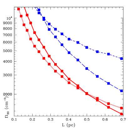
Figure 3: Behavior of the density inferred from the [S ii] lines as a function of the scale $L$ employed in different photoionization calculations (each model is represented by a filled square). The long-dashed and short-dashed line represent two dust-free sequences of models in which the boundary density is $n_{o}=150$ and 2000 ${\rm cm^{-3}}$, respectively. The dotted line and the solid line represent dusty models (all with a boundary density $n_{o}=150$) in which the $orion$ ($\hbox{$\mu_{D}$}=0.8$) or the $noiro$ ($\hbox{$\mu_{D}$}=0.4$) extinction curve was employed, respectively.

0.4 Results of the models

Our main proposition is that only one basic variable of the nebular geometry, the scale $L$, varies behind the slit aperture. We will show that the observations we have taken, albeit very limited, are not inconsistent with this simple picture.

0.4.1 Properties of a powerlaw stratification

For a given dust content $\mu_{D}$ and dust extinction curve, we proceed to show that for a given value of $n_{o}$, there exists a unicity relation between the [S ii] density (which is representative of the IF electronic density) and the scale of the gradient $L$. This is shown in Fig. 3 where we plot the [S ii] density as a function of the powerlaw scale $L$ employed in different photoionization calculations.

In the dust-free case, the long-dashed line corresponds to the sequence of models with $n_{o}=150$ ${\rm cm^{-3}}$ while the short-dashed line corresponds to models with a higher boundary density $n_{o}=2000$ ${\rm cm^{-3}}$. For the denser model, the density gradient is much too shallow since we get a $R_{s}$ of only 0.25 pc in the model with $L=0.7\hbox{\,pc}$. Clearly, the parameter $n_{o}$ plays an important role. Its value can be deduced by requiring that the best model sequence fits simultaneously the observed profiles along the slit in H$\beta$ brightness and in [S ii] density.

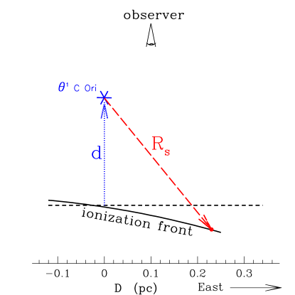
Figure 4: Figure illustrating the sky projection of the West-East aligned slit onto the nebular IF. The distance between $\theta^{1}$ C Ori and the IF is $R_{s}$. The substellar distance is $d$ (see Sect. 0.4.2). There is a further offset of the slit to the South of $\theta^{1}$ C Ori of 0.073 pc (not shown).

In Fig. 3, the dotted line represents the case of using the $orion$ extinction curve with $\mu_{D}$=0.8 (this sequence of models have the same dust characteristics as those assumed by BF91). The use of the smaller grains $noiro$ curve (solid line) on the other hand causes a considerable change in the inferred position of the IF even though these models contain only half the mass of grains present in the $orion$ curve models (dotted line). The reduction of the IF radius is due to the amount of ionizing photons absorbed by the dust grains.

In their determination of the IF shape, WO95 found a very interesting albeit unexplained relationship between the distance to $\theta^{1}$ C Ori and the gas density (their Fig. 6). They also found that the closer the IF is to $\theta^{1}$ C Ori, the higher the H$\alpha$ brightness appears to be. As shown in Fig. 3, a powerlaw stratification establishes a relationship between the scale $L$ and the [S ii] density near the IF. A similar relationship holds between the H$\beta$ surface brightness and the [S ii] density. Our proposed powerlaw stratification is therefore apt in providing a credible explanation to the intriguing [S ii] density-radius correlation discovered by WO95.

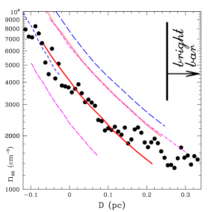
Figure 5: Behavior of the [S ii] density after projection onto our long-slit ($D$ axis). The slit was aligned EW. $D=0$ corresponds to the pixel nearest to $\theta^{1}$ C Ori with $D$ increasing towards the East, crossing the Bright Bar near $D=0.25$. The long and short dash line models represent the dust-free case with $n_{o}=150$ and 2000 ${\rm cm^{-3}}$, respectively. The dotted and the solid lines represent models with internal dust using the $orion$ and $noiro$ curves, respectively (both with $n_{o}=150$). The two dot-dash lines represent the $noiro$ dusty model using an boundary density of $n_{o}=50$ (short-dash dotted line) and 500 ${\rm cm^{-3}}$ (long-dash dotted line), respectively.

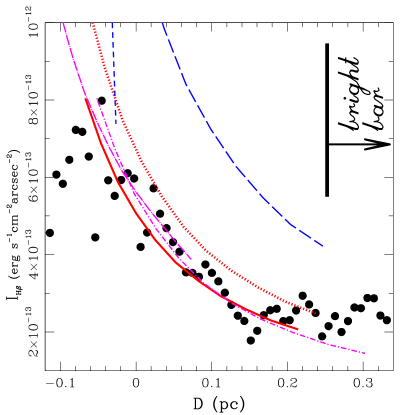
Figure 6: Behavior of the H$\beta$ surface brightness in powerlaw density stratified models after projection onto our long-slit. The long-dash and short-dash lines represent dust-free models with $n_{o}=150$ and 2000 ${\rm cm^{-3}}$, respectively. The dotted and solid line (both with $n_{o}=150$ ${\rm cm^{-3}}$) are models with internal dust using the $orion$ and $noiro$ curves, respectively. The two dot-dash lines represent the $noiro$ dusty model with boundary densities of $n_{o}=50$ (short-dash dotted line) and 500 ${\rm cm^{-3}}$ (long-dash dotted line), respectively. The observed H$\beta$ surface brightnesses plotted here have been reduced to correct for the contribution of the scattered light (Sect. 0.3.3) and for the contribution of the foreground component (Sect. 0.3.2), as in WO95 and BF91, respectively.

0.4.2 Comparison with our long-slit data

Comparison of the models with our long-slit data will be done considering both the [S ii] density and the H$\beta$ surface brightness. One difficulty resides in relating the local IF radius, $R_{s}$, with position, $D$, along our slit. We have proceeded as follows. We have not resolved the inverse problem of finding the distance of the IF at each observed position along $D$. Our main goal consists rather in exploring whether a powerlaw density is generally consistent with the data at hand. With this perspective in mind, we settled for the following simple relation between $D$ and $R_{s}$ : $D=\sqrt{R_{s}^{2}-0.073^{2}\hbox{\,pc}}-d$ where 0.073 pc is the slit offset of 30 to the South, $R_{s}$ the true IF distance to $\theta^{1}$ C Ori for a given slit position $D$ in parsec projected on the sky. $D=0$ corresponds to the pixel nearest to $\theta^{1}$ C Ori with $D$ increasing towards the East. The additional parameter $d$ (in pc) was obtained by iteration, using as constraint that our best model should fit as closely as possible both the observed [S ii] densities and the H$\beta$ surface brightnesses. If the IF lied on a perfect plane perpendicular to our line-of-sight, $d$ would correspond to the substellar distance (O’Dell 1994) and it would have to be subtracted in quadrature from $r$ (as for the slit offset). This resulted, however, in an unsatisfactory fit for all the models tried. A plausible explanation can be found in the 3D-map of the IF shape of WO95 which shows that the IF plane is tilted away from us at the corresponding position of our slit. The above equation, in which $d$ is subtracted linearly, qualitatively describes a tilted plane. A cartoon describing the proposed IF geometry is shown in Fig. 4.

In Fig. 5, we compare our stratified models with the [S ii] densities observed along the slit. For simplicity, all models cover the same range in $L$, from 0.22 to 0.66 pc, which is the appropriate range for the favored solid line model. This has the advantage of clarifying the effect of varying only one parameter at a time (either $n_{o}$ or $\mu_{D}$). The surface brightnesses along the slit are shown in Fig. 6 and can be compared with the various model sequences. The two Figures were drawn using $d=0.26$ which is the value required by the favored model (solid line).

We emphasize that no dust-free model could provide an acceptable fit to the data in both figures 5 and 6, whatever value was used for $d$. In the case of dusty models using the alternative extinction curve $orion$, the fit was never satisfactory in both Figures simultaneously. In effect, if we increase $d$ to 0.35, this shifts all model sequences to the left by 0.09 pc in both Figures, thereby resulting in a good fit of the $orion$ model in Fig 5 but at the expense of an unsatisfactory fit in Fig 6. Increasing the dust content brings the dusty models down but it is not possible in the case of the $orion$ since $\hbox{$\mu_{D}$}=0.8$ is already the maximum allowed given the subsolar metallicity of Orion. The preeminence of small grains, on the other hand, presents the advantage that less dust is necessary ($\hbox{$\mu_{D}$}=0.4$ for the $noiro$ curve). This scenario makes sense in the event that dust grains have been progressively photoeroded.

In conclusion, even when allowing $d$ to vary freely, the Orion model consisting of boundary density $n_{o}=150$ ${\rm cm^{-3}}$ and containing small grains ($noiro$ with $\mu_{D}$= 0.4) provides the optimized set of physical conditions favored by our model for the following reasons:

1. dust-free models are unsuccessful in reproducing the observed behavior of the H$\beta$ surface brightness of Fig. 6 (adopting a larger value for $Q_{H}$ would worsen the discrepancy),

2. for a given dust content and size distribution, the determination of the boundary density $n_{o}$ is straightforward since the curves using different densities lie relatively far apart in the [S ii] density diagram of Fig. 5 (for instance, compare the position of the two dash-dotted lines corresponding to sequences with boundary densities of $n_{o}=50$ or 500 ${\rm cm^{-3}}$),

3. models favoring the preeminence of small grains (e.g. the $noiro$ extinction) provide a simultaneous fit to both data sets presented in Figs 5 and 6, respectively.

The applicability of the proposed model does not include the so-called “Bright Bar” ($\geq 0.25$  pc) beyond which the H$\beta$ brightness is slightly rising. Accounting for this rise in our simple picture would require a gas structure which lies closer to $\theta^{1}$ C Ori than the calculated IF model above. Alternatively, the rise may be due to some sort of limb brightening. Dopita et al. (1974) have proposed for instance that the Bright Bar correspond to the IF seen edge-on. This is qualitatively corroborated by the IF distance map produced by WO95, which shows a sharp ridge at the position of the Bar.

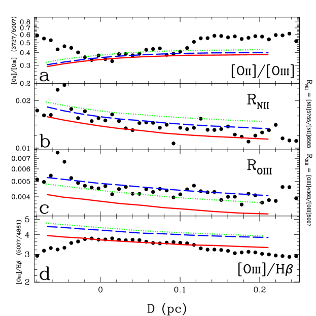
Figure 7: The dots represent the observed line ratios. Panel a: the line ratio [O ii]$\lambda\lambda$3727/[O iii]$\lambda$5007 which is a good indicator of the degree of ionization, panel b: the Nitrogen temperature sensitive ratio [N ii]$\lambda$5755/[N ii]$\lambda$6583, panel c: the Oxygen temperature sensitive ratio [O iii]$\lambda$4363/[O iii]$\lambda$5007, panel d: the [O iii]$\lambda$5007/H$\beta$ $\lambda$4861 ratio. The scale of the 3 panels b, c and d is the same and extend over 0.42 dex. The models (see Sect. 0.4.3): the solid line shows the behavior of line ratios along the slit for our most successful model ($n_{o}=150$ and the $noiro$ curve with $\hbox{$\mu_{D}$}=0.4$). The long-dashed line was calculated assuming temperature fluctuations with $\hbox{$t^{2}$}=0.01$. The dotted line was calculated using half the diffuse field from the “outward-only” approximation. The spike in the data near $D=-0.05$ pc in panels b and c is believed to be due to a foreground proplyd.

0.4.3 Gas temperature and line ratios

Although the current work does not attempt to provide a fit of all the observed line ratios, it is worth checking whether the proposed powerlaw density stratification results or not in ratios similar to the observed. Because the ionization parameter in our models is not a free parameter, line ratios become an interesting consistency check. Furthermore, it is worth testing whether the models can reproduce the observed line ratio trends with slit position.

In a similar fashion to BF91, one important parameter of our models is the stellar temperature which directly affects the excitation line ratio [O iii]/H$\beta$. We found that reproducing satisfactorily this ratio requires a stellar temperature of 38000 K when using the stellar atmosphere models of Hummer & Mihalas (1970). This temperature is consistent with an evolved star of spectral type O7 (c.f. WO95). Our line ratio calculations of [O iii]/H$\beta$ is represented by the solid line in panel d of Fig. 7 using the same parameters as before, that is a boundary density $n_{o}=150$ and an extinction curve consisting of small grains ($noiro$) with $\hbox{$\mu_{D}$}=0.4$. We discuss below possible explanations for the solid line lying slightly below the data. In any event, it is encouraging that the models show the same gradient as the data.

As for the temperature indicators $\hbox{R${}_{{\rm NII}}$}=\hbox{[N\,{\sc ii}]$\lambda$5755}/\hbox{[N\,{\sc ii}]$\lambda$6583}$ and $\hbox{R${}_{{\rm OIII}}$}=\hbox{[O\,{\sc iii}]$\lambda$4363}/\hbox{[O\,{\sc iii}]$\lambda$5007}$, a gradient is also present in the data as shown by panels b and c (BF91 reported also a gradient of R_NII although for a different slit alignment). According to the models, the gradient in the ratio R_OIII is due to a temperature gradient ($\Delta T\simeq 500$ K) while in the case of Nitrogen it is due to both a density gradient (via collisional deexcitation, c.f. BF91) and a temperature gradient. Although the stratified models can successfully fit the observed trends in panels b and c, the predicted ratios lie somewhat lower than observed, more so for R_OIII. Lowering the metallicity would increase R_OIII but at the expense of having the [O iii]/H$\beta$ ratio becoming larger than observed.

It is well known that photoionization models do not explain why the temperatures derived from collisionally excited lines differ from that of recombination lines (see review by Peimbert 1995). In the case of Orion, Esteban et al. (1998) found that the abundance of the O⁺² ion derived from the O ii recombination lines are incompatible with the same ion abundance derived from the collisionally excited [O iii]$\lambda$5007 when a common temperature is adopted. Deriving a unique ionic abundance was found to require different mean temperatures. These can be justified if there exist high amplitude temperature fluctuations in the nebula (Peimbert 1967) which far exceed the amplitude arising from traditional photoionization models (Kingdon & Ferland 1995, 1998; Pérez 1997). The mean square fluctuation amplitudes that Esteban et al. inferred, lie in the range $\hbox{$t^{2}$}=0.02$–0.028. The effect of temperature fluctuations on line emissivities were incorporated in the code mappings ic along the scheme described in Binette & Luridiana (2000). The long-dashed lines in Fig. 7 represent such a model calculated with $\hbox{$t^{2}$}=0.01$. As expected, R_NII and, more so, R_OIII are both significantly increased and can now reproduce satisfactorily the data of panels b and c. The calculated [O iii]/H$\beta$ ratio in panel a, however, lies now too high and the stellar temperature would have to be reduced in order to produce a self-consistent model in all panels. Given our current poor knowledge about the nature and cause of the postulated temperature fluctuations, we have not carried out further the iterative process.

The diffuse ionization radiation field plays a non-negligible impact on the gas temperature. In our models, we use the “outward-only” approximation to treat the transfer of the diffuse radiation. This is equivalent to assuming a single direction for the propagation of the diffuse field, a technique based on the approximation that the diffuse field is soft and does not therefore travel far from the point of emission. To test whether the integration along the direction of increasing density may cause an overestimation of the intensity of the diffuse radiation, we have calculated models in which we reduced by half the strength of the diffuse field (adopting $\hbox{$t^{2}$}=0$). Such models are represented by the dotted-line in Fig. 7. We can see a significant shift which is in the same direction as that caused by temperature fluctuations with $\hbox{$t^{2}$}\sim 0.01$. The dotted line gives us a useful upper limit on the line ratio uncertainties resulting from a possible inadequacy of the outward-only approximation.

Panel a is a plot of the [O ii]/[O iii] ratio. The models can reproduce the observed points only within a restricted slit range. No obvious explanation can be found for the discrepancy outside it. It possibly reflects the limitations of our simplified geometry as discussed in Sect. 0.3.2 or the larger errors affecting the UV [O ii] lines. Overall, the fit of the gradients using our simple models appears satisfactory in all the panels of Fig. 7.

0.5 Conclusions

The method used by WO95 to determine the IF shape requires, at each point of the nebula, knowledge of both the H$\alpha$ surface brightness and the IF density (using the [S ii] or [O ii] doublet). For a powerlaw density stratification as proposed in this Paper, the density across the nebula is not a free parameter since it is uniquely determined by the local powerlaw scale $L$. This opens the possibility that using only the H$\alpha$ (or H$\beta$) surface brightness map, one could in principle determine the IF shape of the whole nebula. For this reason, further studies are warranted in order to: $a)$ extend the comparison of powerlaw density models to a more extensive set of observations of Orion and $b)$ work out a scheme to solve for the inverse problem (as was done by WO95 in the exponential case) in order to determine the IF shape assuming the proposed powerlaw density gradient and taking into account the effects of internal dust.

- [1] Baldwin, J. A., Ferland, G. J., Martin, P. G., Corbin, M. R., Cota, S. A., Peterson, B. M., & Sletteback, A. 1991, ApJ, 374, 580 (BF91)
- [2] Binette, L., & Raga, A. 1990, AJ, 100, 1046 (BR90)
- [3] Binette, L. & Luridiana, V. 2000, RevMexAA, 36, 43
- [4] Binette, L., Wang, J., Villar-Martin, M., & Magis C., G. 1993, ApJ, 414, 535
- [5] Bertoldi, F. 1989, ApJ, 346, 735
- [6] Bertoldi, F., & Draine, B. T. 1996, ApJ, 458, 222
- [7] González-Gómez, D. I. 1999, Tesis de Licenciatura: “Regiones Ionizadas Gigantes”, Universidad Autónoma de Puebla, Puebla (México)
- [8] Dopita, M. A., Dyson, J., & Meaburn, J. 1974, Ap&SS, 28, 61
- [9] Esteban, C., Peimbert, Torres-Peimbert, S., & Escalante, V. 1998, MNRAS, 295, 401
- [10] Franco, J., Tenorio-Tagle, G., & Bodenheimer, P. 1989, \RMAA, 18, 65
- [11] Franco, J., Tenorio-Tagle, G., & Bodenheimer, P. 1990, ApJ, 349, 126
- [12] Franco, J., García-Barreto , A., & de la Fuente, E. 2000a, ApJ, 544, 277
- [13] Franco, J., Kurtz, S., Hofner, P., Testi, L., García-Segura, G., & Martos, M. 2000b, ApJ, 542, 143
- [14] Kingdon, J. B., & Ferland, G. J. 1995, ApJ, 450, 691
- [15] Kingdon, J. B., & Ferland, G. J. 1998, ApJ, 506, 323
- [16] Hester, J. J., et al. 1996, AJ, 111, 2349
- [17] Hillier, D. J., & Miller, D. L. 1998, ApJ, 496, 407
- [18] Hubeny, I., & Lanz, T. 1995, ApJ, 439, 875
- [19] Hummer, D. G., & Mihalas, D. M. 1970, MNRAS, 147, 339
- [20] Magris C., G., Binette, L., & Martin, P. G. 1993, Ap&SS, 205, 141
- [21] Martin, P. G., & Rouleau, F. 1991, in First Berkeley Colloquium on Extreme Ultraviolet Astronomy, (Pergamon Press: New York) eds. R. F. Malina and S. Bowyer, p. 341
- [22] Münch, G. 1958, Rev. Mod. Phys., 30, L1035
- [23] O’Dell, C. R. 1994, Ap&SS, 216,267
- [24] Pauldrach, A. W. A., Hoffmann, T. L., & Lennon, M. 2001, A&A, 375, 161
- [25] Peimbert, M. 1967, ApJ, 150, 825
- [26] Peimbert, M. 1995, in proc. of The Analysis of Emission Lines, ed. R. E. Williams and M. Livio (Cambridge: Cambridge University Press), 165
- [27] Pérez, E. 1997, MNRAS, 290, 465
- [28] Richling, S., & Yorke, H. W. 2000, ApJ, 539, 258
- [29] Rodriguez, M. 1999, A&A, 351, 1075
- [30] Sankrit, R., & Hester, J. J. 2000, ApJ, 535, 847
- [31] Seaton, M. J. 1979, MNRAS, 187, 73P
- [32] Schaerer, D., & de Koter, A. 1997, A&A, 322, 598
- [33] Shields, G. A., & Searle, L. 1978, ApJ, 222, 821
- [34] Stasińska, G., & Szczerba, R. 2001, A&A, 379, 1024
- [35] Tenorio-Tagle, G. 1979, A&A, 7, 59
- [36] Williams, R. E. 1992, ApJ, 392, 99
- [37] Wen, Z., & O’Dell, C. R. 1995, ApJ, 438, 784 (WO95)
- [38] Wurm, K. 1961, Z. Astrophys., 52, 149
- [39] Yorke, H. W. 1986, ARA&A, 24, 49