Around the Clock Observations of the Q0957+561 A,B Gravitationally Lensed Quasar II: Results for the second observing season

Abstract

We report on an observing campaign in March 2001 to monitor the brightness of the later arriving Q0957+561 B image in order to compare with the previously published brightness observations of the (first arriving) A image. The 12 participating observatories provided 3543 image frames which we have analyzed for brightness fluctuations. From our classical methods for time delay determination, we find a $417.09\pm 0.07$ day time delay which should be free of effects due to incomplete sampling. During the campaign period, the quasar brightness was relatively constant and only small fluctuations were found; we compare the structure function for the new data with structure function estimates for the 1995–6 epoch, and show that the structure function is statistically non-stationary. We also examine the data for any evidence of correlated fluctuations at zero lag. We discuss the limits to our ability to measure the cosmological time delay if the quasar’s emitting surface is time resolved, as seems likely.

1 Introduction

An observing campaign to determine the Q0957+561 A,B gravitational lens time delay to a fraction of a day has been undertaken, justified by the evidence available that the quasar has brightness fluctuations on time scales of hours and that microlensing on day timescales is observed (Colley & Schild 1999). Our report (Colley et al. 2002) of the brightness fluctuations observed in Jan 2000 in the first arriving A image becomes a prediction of the pattern of fluctuations expected in March 2001. In this report we present reductions of CCD images for the determination of the B image brightness record, and the determination of a refined value of the time delay.

This time delay determination comes as refinement of previous estimates which have gradually converged to a value near 417 days. After some years of uncertainty whether the delay was near 415 days or 540 days, new estimates have come from new data sets and re-analysis of extensive older data sets to produce values of 416.3 (Pelt et al. 1998), 417.5 (Kundić et al. 1997), $425\pm 17$ (Pijpers 1997), and 417.4 (Colley & Schild 2000). Re-analysis of much of the same data has produced a divergent value of $422.6\pm 0.6$ days (Oscoz et al, 1999) but our present program allows no check on this value because our monitoring was only over a 10 day time interval. Radio brightness monitoring has not had the time sampling, accuracy, or the demonstrated rapid variability to justify participation in this program.

In section 2 we report the new data and reductions for the 12 participating observatories. Section 3 contains an analysis for time delay. We found only a low-amplitude of brightness fluctuations for the quasar during the monitoring period, and any evidence for rapid microlensing is within the noise of our data. However a sharpened value of the time delay allows us to re-analyze high quality data sets from published reports (Colley & Schild, 2000), and a determination of the structure function for the rapid microlensing in that dataset will be the subject of a subsequent report.

2 Observations

Our list of participating observatories was shown as Table 1 of Colley et al. (2002), (Paper 1). For the second season three additional observatories joined the collaboration, principally to cover the Pacific region. The 61cm Mauna Kea reflector was operated from the Institute for Astronomy offices at Hilo, Hawaii. The Mexican 1.5m Harold Johnson Telescope at OAN (Observatorio Astronómico Nacional) at San Pedro Mártir joined the 2.1m OAGH telescope in northern Mexico. The Mt. Megantic telescope in Montreal, Canada provided coverage of the North American continent from a different weather zone.

In this section we provide additional remarks about the data reductions and its relationship to the telescope and camera properties. Any changes from the properties noted in Paper 1 will be given. Our list begins at the international date line and is ordered by increasing longitude. Throughout this section and report, we refer to R filter images only, and although approximately 10% of our data was taken with a V filter we do not remark on the results for this supplementary reduced data set.

2.1 BOAO (S. Korea)

This observatory produced 180 quasar image frames over 5 nights, all of uniformly high quality. The BOAO data from our first year observations are particularly important because they recorded a rapid brightness decline in the A image that will strongly contribute to the present time delay determination. However, as noted in Paper 1, the rapid brightness decline seemed to be recorded in both quasar images and we were suspicious that it might have been the result of some peculiar instrumental effect, although re-reduction of the data with entirely different software seemed to confirm the reality of the rapid brightness change. Thus it is reassuring that the BOAO data in the new campaign seem to again be of high quality and contain no bothersome artifacts evident in the reduced data.

2.2 SOAO (S. Korea)

This 61cm telescope on the top of Mt. Sobak in the middle of South Korea is often differently affected by weather than BOAO, and so is of importance to us because of concern about coverage of the vast Pacific region. The telescope lacks an offset guider, however, and some of the images are streaked slightly. Nevertheless we reduced 236 quasar image frames obtained over 5 nights, albeit with slightly shorter exposure times. The smaller aperture produces lower signal levels, and the error bars for the data set may be seen to be somewhat larger.

However the time coverage by the SOAO observatory has been critical to our program, especially as it provided the only coincident coverage of the rapid brightness decline recorded the previous year at BOAO as noted previously. The relatively large amplitude, approximately 40 milli-magnitudes (mmag) over just 5 hours, adds considerable weight to our time delay determination.

2.3 Maidanak (Uzbekistan)

Since the previous year’s campaign, the Maidanak 1.5m telescope has been equipped with a new CCD camera having $2048\times 800$ pixels and providing an image scale of .121 arcsec/pixel. The images are of the highest quality because of a combination of superb optics and consistently excellent seeing.

We did, however, encounter a problem with the new camera. A large diffuse bright spot of only 3% amplitude covers the entire central region of the CCD frame. The spot is apparently caused by light that is diffusely reflected from the region of the CCD detector back to the camera optics, and then again reflected back onto the CCD camera. This produces an excess brightness near the center of the CCD frame that the standard flat-fielding procedure interprets as locally more sensitive pixels. So in correcting for the apparently high sensitivity of the central region’s pixels, the flat-fielding procedure also reduces the brightnesses of the central stars in the corrected frame. The point is that flat-fielding assumes that all processes affecting the sky brightness across the image frame, such as pixel-to-pixel sensitivity and vignetting, are multiplicative, and a process that adds brightness causes failures and errors in the flat-fielding process. We corrected the problem by preparing an unsharp mask image from a stack of nighttime image frames, and subtracting off the excess brightness from our image frames and flat-field frames before flat-fielding.

The corrected frames have produced an important backbone to our brightness record, because of the consistently high quality and because of the excellent coverage of our monitoring window. The campaign produced 395 image frames over 8 nights in our program.

2.4 TUG (Turkey)

The 1.5m telescope was not equipped with an offset guider, and some images are somewhat streaked but the effect was minimized by taking relatively short exposures. A total of 192 image frames were collected on 6 nights. We were unable to obtain consistent photometry from the images, and we do not believe that the guiding was the problem. Instead, it appears that a slight non-linearity in the camera’s response is indicated. For example, on the cloudiest night, although the quasar brightness is referenced to local field stars, our reduced photometry was several percent different from the photometry on strictly clear nights.

We are hopeful that the data will be reducible after some mapping function of the camera response to light is available. For the present cannot include this otherwise excellent data set in our time delay determination or in the Fig. 1 plot of the brightness curve, at least until we understand better the camera’s slightly non-linear response to light.

2.5 NOT (Canary Islands)

The 2.5m NOT telescope is the largest involved in our campaign and was scheduled for 4 nights which turned out to have nearly ideal weather, producing a harvest of 755 image frames. These have provided excellent photometry and excellent statistics on the four nights, and together with the Maidanak results have produced a “backbone” against which we refer other observatories to look for systematic differences.

2.6 JKT (Canary Islands)

The 1m Johannes Kepler Telescope was scheduled for the last two nights of the formal monitoring period plus two nights beyond to allow some information about the time delay in case the 424-day delay value championed by Oscoz et al. (2001) turn out to be correct. A total of 147 quasar image frames were analyzed and produced a brightness record compatible with results for the other observatories.

2.7 IAC80 (Canary Islands)

The 80cm reflector produced 173 quasar image frames on 8 nights of the formal monitoring period and 3 nights beyond to allow further check on the longer delay value of 424 days advocated by Oscoz et al. (2001). We have not been able to bring the photometric results into agreement with the reductions for other observatories for reasons that we do not yet understand. Most problematic are the results for JD2451983, where the reduced photometry is 2% brighter for image B than for image A as compared to results for the same night from Maidanak and from NOT. Data from the remaining nights seem not to share this defect, and we are puzzled about its origin. Because the images were precisely registered on the CCD detector by an offset guider, it is possible that a CCD defect has affected the photometry for a single night. We have found that pixel-to-pixel sensitivity variations of the CCD detector of 10% are routinely found, and we suspect that the CCD camera is not operated in correct adjustment. We expect to investigate this anomaly further, but for the present analysis we cannot justify censoring a single night’s data only, and for now we have not included the IAC data in our final data compilation and time delay calculation.

2.8 Mt. Megantic (Montreal)

The Mt. Megantic observatory is sited at a very dark mountainous region 250 km east of Montreal, near the U.S. border. It offers a 1.6m Ritchey-Chretien telescope with an offset guider that has been extensively used in photometric programs to date. Over 4 nights the observatory contributed 115 data images of excellent quality to our program.

2.9 Mt. Hopkins (Arizona)

The Mt. Hopkins Observatory has been the mainstay of Q0957 brightness monitoring for over 20 years. Because of scheduling difficulties the 14 nights allocated overlap only 3 nights with the campaign time interval. The additional 11 nights precede the campaign and allow check on possible time delays less than the nominal 417 days. Over 12 nights 375 image frames were reduced for photometry.

2.10 Mexico - 1.5m Harold Johnson Telescope, San Pedro Mártir (Mexico 2)

A total of 126 images over 4 nights were reduced for photometry with this telescope. The images were of excellent quality. The telescope was scheduled for only the first 7 nights of the campaign, with the last 3 nights covered by a second Mexican telescope.

2.11 Mexico - 2.1m Telescope OAGH, Cananea (Mexico 1)

From the OAGH (Observatorio Astrofísico Guillermo Haro) in Cananea, Sonora, a total of 84 image frames were obtained over 2 nights at the end of the monitor period. Very poor (3.5 arcsec) seeing was experienced during part of one night. In general the image quality was not quite as good as the upgraded Harold Johnson 1.5m telescope, likely a result of a problem with the mercury belt of the mirror support system. Nonetheless, the data reduction procedure seems to have produced excellent results for this telescope.

2.12 61cm Mauna Kea Telescope (Hawaii)

The Hawaiian 61cm telescope was operated remotely from the Institute for Astronomy at Hilo and from the University of Hawaii at Honolulu. With clear skies and excellent seeing, a large quantity of data was obtained, but lack of an offset guider caused some trailing of the images. Nevertheless most of the data could be easily reduced with our robust computer program, and the Hawaii telescope produced one of our main data sets. Over 8 nights 430 useful image frames were obtained.

3 Analysis: Data Reduction and Time Delay

The data for all observatories was analyzed by a single program as described in Colley et al. (2002a,b) and in Colley & Schild (1999, 2000). Briefly, all images were de-biased and flat fielded, and the corrected images had the star positions identified from an automatic procedure. Aperture photometry was performed on the two quasar images and several nearby standards, and the quasar brightness was referenced to the standards. Corrections for the aperture crosstalk were determined according to the Colley et al. (2002b) method: a simple parabolic fit to the magnitude relative to the mean magnitude of the run, vs. the log of FWHM seeing is made, and that signal is subtracted out. Colley & Schild (1999) showed that a detailed correction involving galaxy subtraction from HST data (Bernstein et al. 1997) and detailed A-B aperture cross-talk corrections yielded a relation to seeing well described by this very simple model.

The reduced data are shown in Fig. 1, where we plot the photometry obtained in the campaign time frame 12–21 March 2001. Upper and lower plots show the A and B image photometry, and the bottom panel shows as bars the time coverage of each participating observatory, and at the bottom the total coverage. The plotted data points show the hourly photometry means obtained by each observatory, and an error bar calculated from the photon statistics relevant to the detection (not a standard error relative to the mean).

We are frankly disappointed by the low level of brightness fluctuations shown by the late-arriving B image, which will now be compared with the A image data for the previous year. Note that from simple inspection it may be seen that the amplitude of fluctuations in image B is approximately half the level seen in image A for 2001. Similarly, data for image A in 2000 show fluctuations only half as large as those for image B. Both the 2000A and 2001B patterns exhibit less than half the amplitude of the pattern found for fluctuations in 1994–96 by Colley and Schild (2000). Thus the quasar has given us an opportunity to demonstrate that accurate photometry and detection of a very low level amplitude of brightness fluctuations could be produced with our methodology, but we would have preferred stronger fluctuations.

The time delay calculation was undertaken with the “PRH” method (Press et al. 1991), which, despite some controversy has become a standard utility. The method is based on the notion that the quasar variations exhibit a power-law “structure-function,” which is to say the expected magnitude variance of one point from another on the light-curve is power-law in the time separation of the points, (i.e. $V\propto|t_{1}-t_{2}|^{\alpha}$). This method allows one to address the non-uniform time sampling of the data without direct interpolation. From there, usual second-order Gaussian statistical methods are used to construct a “$\chi^{2}$” statistic that reduces to the usual $\chi^{2}$ method if there were no interpolation necessary.

The method is known to have problems, particularly if the data records are affected by microlensing (a highly non-Gaussian signal) (Press & Rybicki 1997, Thomson & Schild 1997, Schild 1996). The method also has a propensity to favor lags where there is the least data overlap (Colley & Schild, 2000), but because our data have an irregular sampling history, this is not expected to be a problem.

Results for the PRH method test are shown in Fig. 2, where we plot $\chi^{2}$ as a function of lag between the A and B images. A small valley for 417.1 days is presumed to indicate the best value of time delay. Toward the left of the plot, the $\chi^{2}$ value declines chiefly because the main feature of the image A light-curve ceases to overlap with the image B’s shifted dates.

The agreement of the two quasar brightness curves for a 417.1-day lag is shown in Fig. 3, where we plot as unfilled circles the image A data from 2000 and as filled circles the image B data from 2001. Error bars are computed as described previously, and are calculated from the fundamental photon statistics, not from the purely empirical departure of individual points from the hourly means. Also shown is the “error snake” that shows the width of the 1-$\sigma$ error interval computed by the PRH method as part of the interpolation scheme. Note that the mean width of this snake is only 5 milli-mag (henceforth mmag, where 1 mmag = .001 mag). A quick glance shows that the true errors seem to be very close to the computed errors, in the sense that more than half the hourly average points lie within the 1-$\sigma$ “snake”.

The formal time delay value calculated for the project is $417.09\;\pm\;0.07$ days. Inspection of Fig. 3 shows that a weak pattern of fluctuations is seen throughout the campaign period, and a single fluctuation at $\mbox{JD}-2449000$ = 2564.5 of 30 mmag amplitude predominates. We suspect that the overall pattern and the single large event contribute about equally to the time delay value. As was noted by Colley et al. 2002a, the event was seen in the Korean/BOAO data from the first season and not entirely believed because the data seemed to show a simultaneous event in the B data for 2000 also. However re-reduction of the data with a different analysis program (IRAF) seemed to show that the feature is real, and its repetition in 2001 make the case more convincing.

With the data in Fig. 3 plotted for the best fit lag, the plot also becomes a record of microlensing, in the sense that any significant differences between the two brightness records indicates a pattern of fluctuations not intrinsic to the quasar, and presumably originating in the lens galaxy. We do not find that the Fig. 3 comparison makes a convincing case that any microlensing has been detected at the 5 mmag level. There is an appearance of a peak for $\mbox{JD}-2449000=2564$, and we note that evidence for this peak comes from two observatories (Maidanak and BOAO.). We have seen evidence for a peak of similar amplitude and duration in the Q0957 B data record for JD 2449704 as illustrated in Fig. 3 of Colley & Schild (2000). The detection of an event in our microlensing record is only based upon 3 hourly average data points, each having approximately $2\sigma$ significance, and we feel obliged to err on the side of conservatism and claim no significant detection.

We do not consider that this proves that rapid microlensing does not exist; our sharpened time delay of 417.1 days will allow us to show from previous data records that data from a single observatory can overlap, and produce microlensing information. This will be the subject of a further report.

4 The Structure Function

In Fig. 4 we show the structure function for the quasar’s brightness fluctuations during Jan 2000 for image A and March 2001 for image B. In Figure 4 the variance plotted as a function of lag is a squared quantity, so the actual brightness fluctuations are the square root of the plotted numbers. Thus for a lag of one day, either image component showed variance of approximately $10^{-5}$, or the mean brightness fluctuation was $0.3\times 10^{-2}$, or 3 mmag. So on average, the quasar brightness changed by only 3 mmag during any 24-hour time interval.

This level of brightness fluctuation is extraordinarily low for this quasar, as may be seen from comparison with the solid line which shows the fit to the variance measured in 1995 (Colley & Schild 2000, Fig. 5). Thus we were extremely unlucky that the date chosen for the beginning of our monitoring for reasons of optimum observability turned out to coincide with a period of low quasar activity. This allowed us to demonstrate the ability to reduce data from multiple observatories and measure brightness with high precision, but we would have preferred to find large fluctuations to firmly establish a time delay and microlensing.

Fig. 4 quantitatively shows that the statistics of the quasar’s brightness fluctuations are highly non-stationary. On timescales of 1–10 days the fluctuations were smaller than measured in 1995; on time scales of a year, the fluctuations were actually twice as large as measured in 1995 (the data point for year lag is far off scale and not seen on this plot).

5 The Correlation for Zero Lag

In the course of monitoring Q0957, many groups have noticed a “zero lag” correlation between the A and B images (e.g., Kundić et al. 1995). This “zero lag” correlation is impossible by all models of the gravitational lensing, and would require some kind of precisely aligned gravitational wave in the Halo of our Galaxy or perhaps a cosmic string. It is presently interpreted as a frame-by-frame correlated error in the photometry.

The Kundić et al. (1995) group endeavored with fair diligence to uncover the source of such an error, examining moon phase, zenith angle, and many other observational states for some correlation with the apparent photometric errors, but encountered little success. We have also noticed that our data seem, upon inspection, to exhibit a similar “zero lag” correlation, even after our parametric correction for seeing, discussed previously. In particular, the PRH “snake,” a completely objective interpolation, yields light-curves in which the coincidence of the many shallow peaks and valleys is immediately striking to the eye. We therefore engaged ourselves in a great amount of effort to remove errors that might be correlated with flux, sky background, location on CCD, and time of night, but those efforts have yielded little improvement for most observatories.

We show the effect quantitatively in Fig. 5 as the PRH $\chi^{2}$ (lower $\chi^{2}$ means higher correlation) for lags in the vicinity of zero lag in the two data sets; the solid curve shows the correlation for the 2001 data, and the dashed curve shows the correlation for 2000. Any correlations would be expected to be quite random in the vicinity of zero lag if the photometry were perfect. However, in both cases, there is a $\chi^{2}$ trough near zero. For 2001, the overall minimum is at precisely zero lag, quite suggestive of a photometric problem. For 2000, the case is more muddled. The trough nearest zero is closer to 0.1 days and is only the sixth lowest trough, while the overall minimum is at around a one day lag. While in the 2001 dataset, there seems to be compelling evidence of a photometric problem, nothing compelling arises in the 2000 dataset, despite identical photometric reduction methods.

Most likely, there is a similar photometric error correlation in both 2000 and 2001, but the true correlation of the light-curves adds slight destructive and constructive interference to that signal (respectively). We interpret Fig. 5, therefore, as showing a zero lag correlation that is evidence of an as yet uncorrected photometric problem at the few mmag level, residing on top of the true correlation (PRH $\chi^{2}$) of the A and B light-curves.

6 The Possibility of Multiple Time Delays

Our brightness monitoring has produced a time delay of $417.09\pm 0.07$ days, and scant evidence for microlensing. During our monitoring campaign the quasar was experiencing below-normal brightness variability, and very possibly the low level of microlensing fluctuations measured is related.

At the time this project was organized, time delays for the gravitational lens system seemed to be converging to a value near 417 days. Analysis of the 17-year brightness history by Pelt et al. (1998) produced a delay of $416.3\pm 1.7$ days, and the Kundic et al. (1997) observation of a large event seemed to make their 417.4 day delay unquestionable, although in hindsight the quoted value was for g-filter data, and their r-filter data gave 420.3 days. Finally the extensive monitoring over 7 consecutive nights reported in Colley & Schild (1999) seemed to make a convincing case that significant fluctuations were observed, and repeated after a time delay of 417.4 days. Their Fig. 7 appeared to show ample repeated fluctuations to define adequately the time delay.

At the same time, suspicions of a somewhat longer time delay have arisen. The Pijpers time delay determination using a long extensive data base gave $425\pm 17$ days, but the error seemed to include the favored shorter value. But then a report by Oscoz et al. (2001) seemed to show a longer delay for the same data sets, utilizing different statistical methods. A new thesis by Ovaldsen (2002) with re-reduction of the original data frames seems to show not only stronger evidence for the 424-day delay, but even a small local anti-correlation bump in the delay curve where the favored 417-day lag should be. Thus we find it perplexing and frustrating that with so many nights of overlapping data, it is difficult to find an enduring time delay.

As noted by Pelt et al. 1996, the fine structure filtered out of the brightness record does not give a time delay value (Pelt et al. 1996, Fig. 10, 11), even though hundreds of nights of data overlap for any test value of lag near 420 days (Pelt et al. 1996, Fig. 1). If microlensing were not affecting the brightness records, it should be easy to determine the time delay to a fraction of a day.

We believe that it is now appropriate to re-assess our assumptions and methodology to ask what we are seeking and why we have such problems finding it. We seek the time delay between the propagation paths for the two quasar images, where it has long been believed that the geometry of the smooth mass distribution in the direction of the lens system provides different paths and the two quasar images are seen at different times. We have presumed that by observing brightness fluctuations of the two images we will be able to match up the patterns and measure the time delay. But what are the limits to this procedure if the quasar’s luminous structure is so large that microlensing by massive objects in the lens galaxy amplifies different parts of the quasar by different amounts? What if, for example, the inner edge of the accretion disc is highly microlensed for the A image but not for B?

For the Q0957 radio source quasar the black hole mass would be perhaps $3\times 10^{9}M_{\odot}$, giving a Schwarzschild diameter of $2\times 10^{15}$ cm. Thus the diameter of the innermost stable orbit, $6R_{S}$, is approximately $10^{16}$ cm, or 4 light days. For a quasar redshift of 1.4, a proper time of 4 light days is observed as 10 days. As such, a maximum of 1% variability might be expected on the timescale of hours (pertinent to this paper). Colley & Schild (1999) showed by measuring the structure function down to sub-day lags, that more typically the quasar varies about 1% per day on average.

With an inner diameter for the accretion disc of order 10 days (our time), a simultaneous event that illuminated the entire inner disc would appear to us to brighten roughly 10 days earlier on the front size compared to the back side. This simple light travel time couples strongly to the microlensing. By coincidence, the Einstein radius (at the source), is also of order $10^{16}\;\mbox{cm}$ for stellar mass objects in the lens galaxy. In this high optical depth case, the Einstein radius becomes the typical separation between caustics. Thus, if the stars alone had an optical depth of order 0.1, of order 10% of the time one would expect a caustic to be lying somewhere on the inner accretion disc. Hence, one image could significantly magnify the same event at a different time than the other, due to simple light travel time from one edge of the QSO emitting surface to the other.

Since the inner edge of the disc presumably demonstrates a significant fraction of the variability seen on the few-week timescale (typical of the large events seen in the QSO historically, including those leveraged for time-delay measurements [e.g., Kundić et al. 1997]), a light travel time problem could be significant even without a MACHO dark matter population. If there is a significant population of MACHOs, the problem becomes nearly unavoidable.

Additional outer structure at scales of 100 days (our time) is implied in the Elvis (1999) model. If such structure responds to an event near the center, the light travel time problems are exacerbated, particularly for stellar mass lenses, since one would expect multiple caustics to lie somewhere on this outer structure all the time. Thomson & Schild (1997) encountered autocorrelation peaks near 100 proper light days, which supports the Elvis (1999) model. Such a model would necessarily present substantial light travel time signal in the light curve.

Further evidence for the phenomenon comes from a cross-correlation calculation for Q0957 by Schild and Cholfin (1986), who showed a Full Width at Half Maximum (FWHM) of nearly 100 days; subsequent analyses of the same or comparable data sets by Vanderriest et al. (1989) and Press, Rybicki, and Hewitt (1991) gave a similar result. Even the modern calculations by Pelt et al. (1997) shows in their Fig. 3 and following figures a 100-day wide correlation curve. Only the more modern calculations for short data sets centered around strong brightness changes give the sharper cross-correlation peaks of programs by Kundić et al. (1997) and Colley & Schild (1999). Thus, quasar structure on observed scales of 100 light-days (observed) has long been predicted by observations.

More significant results were gleaned from a statistical analysis of the brightness records by Thomson & Schild (1997) who found two unexpected facts. Their Fig. 6 shows that different subsets of the brightness data show different lags, with the lags seeming to persist over approximately 2 years. This would be expected if microlensing were locally magnifying different parts of the quasar’s luminous region by different amounts as the pattern of microlenses changes on a time scale of 2 years. Furthermore, their Fig. 3 seems to show autocorrelation peaks with observed lags near 200 days, suggesting that the quasar has some structure on scales much larger than the 1-night sampling of most data. (note that for a quasar at $z=1.4$, the proper scale of the implied quasar structure is 200 days / 2.4, or approximately 70 light day proper size scale.) Weaker structure on smaller scales is further implied by autocorrelation peaks near 20 light days (observed).

Thus we interpret our new time delay measurement as follows. For the microlensing configuration observed in calendar 2000–01, the time delay corresponding to the microlensing alignment then relevant is 417.1 days. Possibly other parts of the quasar were being magnified to produce other lags as well, but their signature is hardly apparent because of the disappointingly low level of quasar activity. Very probably a component of what is commonly called rapid microlensing is actually the result of quasar brightness fluctuations seen magnified by the different microlensing of the A and B images, and any other data sets taken at epochs close to ours might well find evidence for other lags. Our 417.1-day lag is sharply defined by the depth and narrowness of the valley of our PRH autocorrelation calculation, but it does not allow prediction of lags that will be observed several years in the future. Use of this lag will allow us to make careful comparisons of older data sets and allow some conclusions to be made about the structure function for rapid microlensing, which will relate to both the quasar’s structure and the microlensing population.

7 Conclusions and Discussion

We have carried out the first gravitational lens time delay measurement from data sampled nearly continuously over many days. The measurement of $417.09\pm 0.07$ is certainly consistent with many previous efforts (e.g., Kundić et al. 1997), but puzzlingly inconsistent with others (e.g., Oscoz et al. 2001). Since there was surprisingly little variation in the brightness of the QSO images, compared to previous structure function measurements (Colley & Schild 2000), the time delay measurement is not as strong as we had hoped. Furthermore, there is little evidence of microlensing on timescales of hours to days.

In recognizing that there are now (again) two credible, and competing time delays (around 417 days and around 424 days), both with a wealth of evidence to support them, one must attribute the discrepancy either to a lack of quality data, as was done a decade ago (PRH), or to the possibility that the QSO and lens system form multiple delays which foil our efforts to produce a unique time delay. The former seems increasingly untenable given the level of observational effort poured into this system over the past decade. If the multiple delay hypothesis is to be examined, careful consideration of more complex QSO models must be undertaken (e.g., Wyithe & Loeb 2002).

As a final comment, we note that one of the most intriguing aspects of this work has been the formation of a large, international collaboration, and integration of data from widely varying nations, telescopes and instruments. As the number of lensed QSOs has grown, so has the need for nearly constant monitoring by as many telescopes in as many locations as possible, with some coordination. Our project has demonstrated proof that a large international collaboration of medium-sized observatories can be coordinated sufficiently to obtain nearly constant monitoring of lensed QSOs.

Figure 1: The R-band light curve of Q0957+561A,B from March 12 to March 21, 2001. At top is the image A brightness record; in the middle is the image B brightness record, and at bottom is a series of line density graphs illustrating when each observatory was contributing data.

Figure 2: The PRH $\chi^{2}$ calculated as a function of lag for the QuOC1 and QuOC2 data. According to theory, the minimum of this curve occurs for the most probable lag, and thus is a determination of the time delay. Notice that the curve is reasonably symmetrical around the 417.1 day minimum.

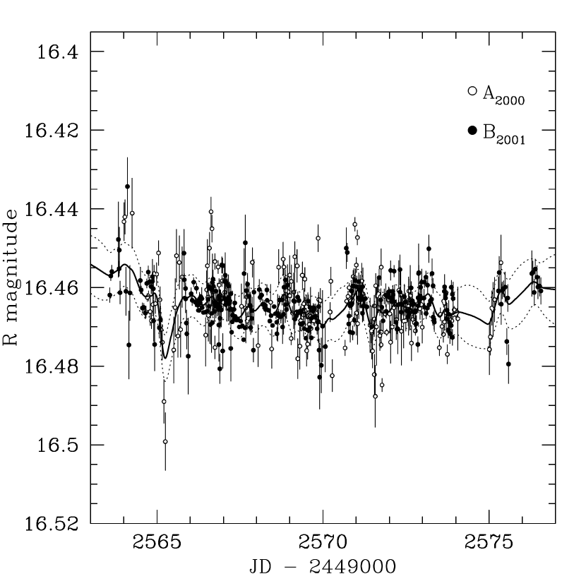
Figure 3: The comparison of brightness fluctuations measured for image A during Jan 2000 (open circles) with fluctuations measured for image B in March 2001 (filled circles), for a 417.1 day lag. Any significant differences would be evidence for microlensing. The error “snake” corresponds to expected $1\sigma$ departures from a mean trend, according to Gaussian statistics.

Figure 4: The structure function for the observed quasar brightness fluctuations. Filled circles show the structure function for image A brightness in Jan 2000, and open stars are for B in March 2001. The solid curve shows the structure function measured by Colley and Schild (2000) for 1995 data. Because the circles and stars seem to agree so well, we presume that plotted points show that the quasar brightness fluctuations estimated in the two seasons agree, but the trend of the new data are significantly different from the 1995 data. This indicates that the quasar brightness fluctuations are statistically non-stationary. Note that the new point for lags near 1 year are far off scale and are not plotted, again a product of the non-stationary statistics.

Figure 5: The cross-correlation for zero lag. Careful inspection of Fig. 1 shows a surprising agreement of the many small peaks and valleys of the objectively measured mean brightness records at zero lag. A similar but less pronounced effect is seen for the QuOC1 data for Jan 2000. Thus we plot the PRH method calculation separately for the Jan 2000 data (dashed curve) and for the March 2001 data (solid curve). Note that 2000 data are fewer in number and the curve has been shifted upward to fit on the $\chi^{2}$ scale for 2001. A minimum with a FWHM of 4 hours is found for data in both seasons, but local minima are also found for $\pm$ 1 and $\pm$ 2 days.

References

- (1)
- (2) Bernstein, G., Fischer, P., Tyson, J. A., & Rhee, G., 1997, ApJ483, L79
- (3)
- (4) Colley, W. N., Shapiro, I. I., Pegg, J., & Jenkins, A. 2002b, ApJ(submitted)
- (5)
- (6) Colley, W. N., & Schild, R. E. 2000, ApJ, 540, 104
- (7)
- (8) Colley, W. N., & Schild, R. E. 1999, ApJ, 518, 153
- (9)
- (10) Colley, W. N. et al. 2002a, ApJ, 565, 105
- (11)
- (12) Elvis, M., 2000, ApJ, 545, 63
- (13)
- (14) Kundic, T. et al. 1997, ApJ, 482, 75
- (15)
- (16) Kundic, T. et al. 1995, ApJ, 455, L5
- (17)
- (18) Oscoz, A. et al. 2001 ApJ, 552, 81
- (19)
- (20) Ovaldsen, J., 2002, Thesis, University of Oslo, http://www.astro.uio.no/ jeovalds/th.html
- (21)
- (22) Pijpers, F. P., 1997, MNRAS, 289, 933
- (23)
- (24) Pelt, J., Kayser, R., Refsdal, S., & Schramm, T., 1996, A&A, 305, 97
- (25)
- (26) Pelt, J., Schild, R., Refsdal, S., & Stabell, R., 1998, A&A, 336, 829
- (27)
- (28) Press, W. H., Rybicki, G. B., 1997, “Astronomical Time Series,” Eds. D. Maoz, A. Sternberg, and E.M. Leibowitz, [Dordrecht: Kluwer], p. 61.
- (29)
- (30) Press, W. H., Rybicki, G. B., & Hewitt, J. N., 1992, ApJ, 385, 404 (PRH)
- (31)
- (32) Schild, R., 1996, ApJ, 464, 125
- (33)
- (34) Schild, R., & Cholfin, B., 1986, ApJ, 300, 209
- (35)
- (36) Thomson, D. J., & Schild, R. 1997, “Applications of Time Series in Astronomy and Meteorology”, ed. T. Subba Rao, [Chapman and Hall: New York], p. 187
- (37)
- (38) Vanderriest, C. et al. 1989, A&A, 215, 1
- (39)
- (40) Wyithe, S. , & Loeb, A., 2002, astro-ph/0204529
- (41)
- (42) Yonehera, 1999, ApJ519, L31-34, 1999
- (43)