Correlation between galaxies and QSO in the SDSS:
a signal from gravitational lensing magnification?

Abstract

We report a detection of galaxy-QSO cross-correlation $w_{GQ}$ in the Sloan Digital Sky Survey (SDSS) Early Data Release (EDR) over $0.2-30$ arc-minute scales. We cross-correlate galaxy samples of different mean depths $r^{\prime}=19-22$ ($\overline{z}_{G}=0.15-0.35$) with the main QSO population ($i^{\prime}_{Q}<19.1$) at $\overline{z}_{Q}\simeq 1.6$. We find significant positive correlation in all cases except for the faintest QSOs, as expected if the signal were due to weak lensing magnification. The amplitude of the signal on arc-minute scales is about $20\%$ at $\overline{z}_{G}=0.15$ decreasing to $10\%$ at $\overline{z}_{G}=0.35$. This is a few times larger than currently expected from weak lensing in the $\Lambda$CDM models but confirms, at a higher significance, previous measurements by several groups. When compared to the galaxy-galaxy correlation $w_{GG}$, a weak lensing interpretation indicates a strong and steep non-linear amplitude for the underlaying matter fluctuations: $\sigma\simeq 400$ on scales of $0.2$ Mpc/h, in contradiction with non-linear modeling of $\Lambda$CDM fluctuations. We also detect a normalized skewness (galaxy-galaxy-QSO correlation) of $S_{3}\simeq 21\pm 6$ at ${\overline{z}}\simeq 0.15$ ($S_{3}\simeq 14\pm 4$ at ${\overline{z}}\simeq 0.35$), which several sigma low as compared to standard $\Lambda$CDM expectations. These observational trends can be reconciled with lensing in a flat $\Lambda$ universe with $\sigma_{8}\simeq 1$, provided the linear spectrum is steeper ($n\simeq 1$) than in the $\Lambda$CDM model on small (cluster) scales. Under this interpretation, the galaxy distribution traces the matter variance with an amplitude that is 100 times smaller: ie galaxies are anti-bias with $b\simeq 0.1$ on small scales, increasing to $b\simeq 1$ at $\simeq 10$ Mpc/h.

1. Introduction

Weak gravitational lensing by foreground large-scale matter density fluctuations could introduce significant density variations in flux-limited samples of high redshift objects, such as QSOs. This is sometimes called magnification bias or cosmic magnification. In principle, it is possible to separate the intrinsic density fluctuations in QSO samples from the weak lensing magnification signal by cross-correlating the QSOs with a low redshift galaxy sample. This allows a direct measurement of how the galaxy distribution traces the underlaying mass distribution. Much work have been done in this direction both on theory and observations (for recent reviews see Norman & Williams 2000, Bartelmann & Schneider 2001, Benitez et al. 2001, Guimarães, van de Bruck and Brandenberger 2001).

Correlation of low redshift galaxies and high-redshift AGNs or QSOs typically find significant excesses of foreground objects around the QSO positions (Seldner & Peebles 1979, Tyson 1986; Fugmann 1988,1990; Hammer & Le Févre 1990; Hintzen et al. 1991; Drinkwater et al. 1992; Thomas et al. 1995; Bartelmann & Schneider 1993, 1994; Bartsch, Schneider, & Bartelmann 1997; Seitz & Schneider; Benítez et al. 1995; Benítez & Martínez-González 1995, 1997; Benítez, Martínez-González & Martín-Mirones 1997;Norman & Impey 1999;Norman & Williams 2000). See also Burbidge et al. 1990 (and references therein) for individual associations and different statistical indications. On the other hand, there has also been reports of significant anti-correlation between galaxy groups and faint QSOs (see Croom & Shanks 1999 and references therein) which could also be explained by weak lensing magnification because of the flater slope of the faint QSO number counts. Even though the shape of the galaxy-QSO cross-correlation has not yet been well constrained, these results seem qualitatively in agreement with the magnification bias effect, but the amplitude of the correlation is found to be higher than that expected from gravitational lensing models based on $\Lambda$CDM.

What is the origin of this discrepancy? Part of the problem could be due to the lack of well-defined and homogeneous samples. After all we are looking for a small effect, may be as low as $1\%$, and any systematics in the sample definition is likely to introduce cross-correlations at this level (see §2 below). On the other hand we know little about clustering of dark matter on sub-megaparsec scales. Could the discrepancy be due to real deviations from the $\Lambda$CDM paradigm?

Recently, Ménard & Bartelmann (2002) and Ménard, Bartelmann & Mellier (2002) have explored the interest of the SDSS to cross-correlate foreground galaxies with background QSO. The SDSS collaboration made an early data release (EDR) publicly available on June 2001. The EDR includes around a million galaxies and 4000 QSOs distributed within a narrow strip of 2.5 degrees across the equator (see Stoughton et al 2002 for details). As the strip crosses the galactic plane, the data is divided into two separate sets in the North and South Galactic caps. The SDSS collaboration has presented a series of analysis (Zehavi et al. 2002, Blanton et al. 2002, Scranton et a.l 2002, Connolly et al. 2002, Dodelson et al. 2002, Tegmark et al. 2002, Szalay et al. 2002, Szapudi 2002) of large scale angular clustering on the North Galactic strip, which contains data with the best seeing conditions in the EDR. Gaztañaga (2002a, 2002b) presented a first study of bright ($g^{\prime}\simeq 20$) SDSS galaxies in both the South and North Galactic EDR strip, centering the analysis on the comparison of clustering to the APM galaxy Survey (Maddox et al. 1990).

In this paper we will follow closely Ménard, Bartelmann & Mellier (2002, MBM02 from now on) proposal to study the galaxy-QSO cross-correlation signal in the EDR/SDSS. The paper is organized as follows. In section §2 we present the samples used and the galaxy and QSO selection. Section §3 is dedicated to the extinction contamination. Section §4 and §5 presents the main results and its interpretation, while §6 and §7 are dedicated to a discussion and a listing of conclusions.

2. QSO and galaxy Samples

The galaxy samples are obtained from the EDR and converted into pixel maps of different resolutions as described in Gaztañaga (2002a,2002b). We select objects from an equatorial SGC (South Galactic Cap) strip 2.5 wide ($-1.25<DEC<1.25$ degrees.) and 66 deg. long ($351<RA<56$ deg.), which will be called EDR/S, and also from a similar NGC (North Galactic Cap) 2.5 wide and 91 deg. long ($145<RA<236$ deg.), which will be called EDR/N. These strips (SDSS numbers 82N/82S and 10N/10S) correspond to some of the first runs of the early commissioning data (runs 94/125 and 752/756) and have variable seeing conditions. Runs 752 and 125 are the worst with regions where the seeing fluctuates above 2”. Runs 756 and 94 are better, but still have seeing fluctuations of a few tenths of arc-second within scales of a few degrees. These seeing conditions could introduce large scale gradients because of the corresponding variations in the photometric reduction (eg star-galaxy separation) that could manifest as large scale number density gradients (see Scranton et al 2001 for a detail account of these effects). We will test our results against the possible effects of seeing variations, by using a seeing mask (see §3.1).

Redshift targets in the SDSS are selected in $r^{\prime}$ for galaxies and $i^{\prime}$ for QSO. Here we use $i^{\prime}$ for QSO and both $i^{\prime}$ and $r^{\prime}$ for galaxies. The first choice has the interest that both galaxies and QSO come from the same photometric reduction and are therefore subject to similar systematics. Galactic extinction is also smaller in this band. The second choice provides a comparison with previous results on galaxy clustering. To maximize the number of galaxies, and therefore the possibility of lensing, we choose broad magnitude bands. We will focus our results in comparing a nearby sample $r^{\prime}=19-17.5$ ($\overline{z}\simeq 0.15$) with a distant one $i^{\prime},r^{\prime}=22-17.5$ ($\overline{z}\simeq 0.35$). Galaxies selected with $i^{\prime}<22$ are almost the same (within few percent) to galaxies in $r^{\prime}<22$ as the K-correction cancels out with the color evolution (see Fukugita et al. 1996). Here we take the $i^{\prime}<22$ band as our nominal choice to minimize extinction (this will give larger area coverage, see below). As we will show, both galaxy-galaxy and galaxy-QSO cross-correlations turn out to be almost identical in $i^{\prime}<22$ and $r^{\prime}<22$, the only difference being slightly smaller errors in the $i^{\prime}<22$ sample. For the bright sample we stick to $r^{\prime}<19$ to provide a more direct comparison with previous results on galaxy-galaxy clustering. Using the redshift distributions in Dodelson et al. (2002), the mean redshift for $17.5<r^{\prime}<19$ (with $\simeq 81000/117000$ galaxies) is $\overline{z}\simeq 0.15$, while $17.5<i^{\prime},r^{\prime}<22$ (with $\simeq 480000$ galaxies within our mask) have $\overline{z}\simeq 0.35$. We will center our analysis over these two samples, which will be sometimes refered to as $r^{\prime}<19$ and $i^{\prime}<22$.

The 1st and 3rd slices in Figure 1 shows the EDR/S and EDR/N pixel maps for $i^{\prime}<18.5$ and $7$ arc-minute resolution. Note the ”barrel” shape in the EDR/N. As far as we have been able to find out, this seems an unreported artifact in the EDR redshift sample release which does not seem to include redshifts for secondary targets in this equatorial strip (see Stoughton et al 2002 for details). This is not a problem in our analysis other than we are missing a good fraction of the EDR/N because there are no matching redshifts for the QSOs. The top slice in Figure 2 shows a zoom over the central region of EDR/N.

We recovered the QSO sample form the SDSS/EDR as described in detailed in Schneider et al (2002, see also Richards et al. 2002). We use point-spread function magnitudes for QSO (which will be quoted with a subindex: $i^{\prime}_{Q}$) and Petrosian magnitudes for galaxies (which will be quoted without any subindex: ie $i^{\prime}$), as indicated by above references. We have considered two QSO samples. The one obtained directly from the EDR data archive (ie just with $\rm specobj.specClass=3$) containing 4275 QSOs, which we call EDR/QSO, and the corrected public QSO sample presented in Schneider et al (2002), which we called SDSS/QSO and contains 3814 QSOs. Almost all SDSS/QSO is contained in EDR/QSO. SDSS/QSO contains a handful of additional BALQSOs and some quasars that were identified by eye during the checking process. SDSS/QSO excludes most of the low-redshift AGN ($M_{i}<-23$) and a small number of narrow-line QSO included EDR/QSO, but this makes little different for our sample which has $z>0.8$.

Out of the EDR/QSO sample we impose two further cuts: $\rm specobj.zStatus>2$ to exclude failed or inconsistent redshifts and $\rm specobj.zConf>0.7$ to exclude redshifts with confidence less than $70\%$ (see Stoughton et al. 2002 for details). In both samples we restrict our analysis to $0.8<z<2.5$ where the QSO distribution is compact and homogeneous (the lower cut avoids overlap with the galaxy sample). After these cuts the main difference between EDR/QSO and SDSS/QSO are the few missing radio QSO and a few narrow-band emission QSO’s. Over $97\%$ of the QSOs are the same and have the same parameters. Note that according to Schneider et al. 2002, QSO selection criteria were changed systematically during the EDR runs resulting in large variation on the number of QSOs per field. Nevertheless both samples are photometrically completed to better than $90\%$ in $16.5<i^{\prime}_{Q}<19.1$ (Schneider et al. 2002, Stoughton et al. 2002). We will therefore restrict our analysis to $16.5<i^{\prime}_{Q}<19.1$ and further compare results for the two versions of the target selection that are relevant to our sky coverage: v2.2a and v2.7 (see Stoughton et al. 2002).

Number counts and the redshift distribution are shown in Fig.4. Note the sharp break in the QSO number counts at $i^{\prime}_{Q}\simeq 19$. The short-dashed line shows a power law with $10^{0.4m}$ (which corresponds to $\alpha=1$ in Eq.[25]). As lensing magnification should be negative for shallower slopes, we cut the QSO sample to $i^{\prime}_{Q}<18.8$ (which contains $952$ QSOs for $0.8<z<2.5$ within our mask) and use the fainter cut $i^{\prime}_{Q}>18.8$ data (which contains $671$ QSOs within our mask) for comparison. Thus, unless stated otherwise, QSO are selected with $16.5<i^{\prime}_{Q}<18.8$, which for brevity will be sometimes refered as $i^{\prime}_{Q}<18.8$.

Right panel in Fig.4 shows how the redshift distribution for $i^{\prime}_{Q}<18.8$ of EDR/QSO (histogram) and SDSS/QSO (dashed line) are almost identical, with a mean redshift of $\overline{z}_{QSO}=1.67$. The redshift distribution for $i^{\prime}_{Q}<19.1$ is very similar (with just higher surface density). Here we will only present results based on EDR/QSO. We have done all the analysis for SDSS/QSO and find identical results in all cases. We choose to present EDR/QSO because it has been automatically produced (in the same pipeline as the galaxies) and because we are not concerned with the astrophysical nature of the QSO in the sample but rather with having a well defined photometric sample of distant objects.

Figure 1 compares the galaxy pixel maps $i^{\prime}<18.5$ with the QSO $i^{\prime}_{Q}<18.8$ distribution in the same portion of the sky (QSOs are the 2nd and 4th slices below the corresponding EDR/N and EDR/S galaxies). Figure 2 shows a zoom over the central region of EDR/N. Note that there is no apparent correlation between QSO and galaxies. As we will see below, most of the signal we are seeking for is hidden below the pixel resolution of this map.

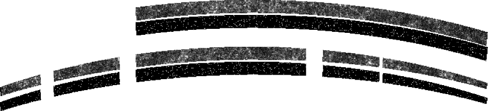
Figure 1.— Equatorial projections galaxy and QSO maps. The top pair of slices correspond to galaxy and QSOs in SDSS EDR/S ($2.5\times 60$ sqr.deg). The bottom two slices shows galaxies and QSOs in SDSS EDR/N ($2.5\times 90$ sqr.deg).

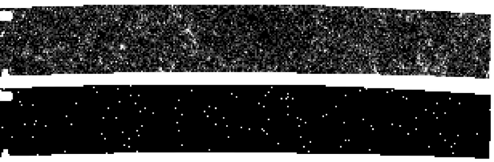
Figure 2.— Zoom over the central part of the SDSS EDR/N (bottom slices in previous Figure).

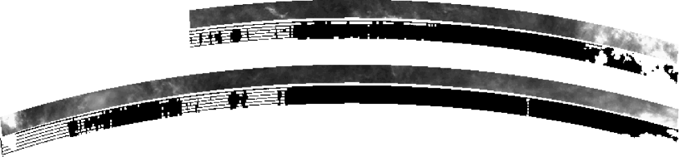
Figure 3.— Pixel maps of galactic absorption (Schlegel et al. 1998) over the EDR/N (top two slices) and EDR/S region. We also show below each extinction map the EDR/SDSS mask of pixels with less than $0.2$ mag extinction in $i^{\prime}$ and less than $2"$ seeing.

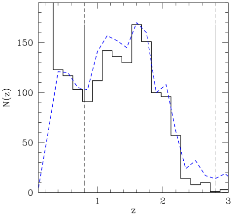
Figure 4.— Left: Integreted QSO number counts per unit magnitude and area. Right: Redshift distributions for the EDR/QSO sample (continuous line) and the SDSS/QSO sample (dashed lines). In both case $16.5<i_{Q}^{\prime}<18.8$.

3. Correcting for Galactic extinction

Absorption by Galactic dust can lead to a positive correlation between galaxies and high-z QSOs (see Norman & Williams 1999). Schlegel et al. (1998) extinction maps have a significant differential extinction $E(B-V)\simeq 0.02-0.03$ even at the poles. Thus, the extinction correction has a large impact in the number counts for a fix magnitude range. The change can be roughly accounted for by shifting the mean magnitude ranges by the mean extinction. Despite this, extinction has little impact on clustering, at least for $r^{\prime}<21$ (see Scranton et al. 2001 and also Tegmark et al. 1998). This is fortunate because of the uncertainties involved in making the extinction maps and its calibration. Moreover, the Schlegel et al. (1998) extinction map only has a 6’.1 FWHM, which is much larger than the individual galaxies and QSO we are interested on. Many dusty regions have filamentary structure (with a fractal pattern) and large fluctuations in extinction from point to point (ie see Fig.3). One would expect similar fluctuations on smaller (galaxy size) scales, which introduces further uncertainties to individual corrections. As we are looking for a very low signal (of order of $1\%$) we have to be very careful with small systematic effects, such as extinction.

The net effect of extinction is to produce a magnitude absorption $A$ which translates into a change in the local galaxy surface number density $N$:

$$\Delta_{A}\equiv{\Delta N\over{N}}\simeq\alpha A$$ (1)

where $\alpha$ is the slope of the number density counts: $N\simeq 10^{\alpha m}$ as a function of magnitude $m$. If the absorption $A$ were a constant, this will would only change the mean number density in an uniform way. Unfortunately extinction is highly variable and produces density fluctuations in the sky:

$$\delta_{A}\equiv\Delta_{A}-<\Delta_{A}>=\alpha\left(A-<\Delta_{A}>\right)$$ (2)

We thus see that extinction will introduce spurious number density fluctuations in both the galaxy and the QSO distributions:

$$\overline{\delta}_{G} = \delta_{G}+s_{G}~{}\delta_{A}$$ (3)

$$\overline{\delta}_{Q} = \delta_{Q}+s_{Q}~{}\delta_{A}$$ (4)

where $\overline{\delta}_{G}$ and $\overline{\delta}_{Q}$ stand for the total observed fluctuations (as opposed to the intrinsic ones, $\delta_{G}$ and $\delta_{Q}$) and $s_{G}$ and $s_{Q}$ are constant numbers characteristic of each population. From the above analysis we can see that extinction will introduce artificial cross-correlations between the galaxy and QSO populations, even when they are intrinsically uncorrelated. One can correct for this type of effects by using the absorption maps. We can calculate the cross-correlations:

$$<\overline{\delta}_{G}~{}\delta_{A}> = s_{G}~{}<\delta^{2}_{A}>$$ (5)

$$<\overline{\delta}_{Q}~{}\delta_{A}> = s_{Q}~{}<\delta^{2}_{A}>$$ (6)

$$<\overline{\delta}_{G}~{}\overline{\delta}_{Q}> = <\delta_{G}~{}\delta_{Q}>+s_{G}~{}s_{Q}~{}<\delta^{2}_{A}>$$ (7)

where we have assumed that the intrinsic galaxy and QSO positions are uncorrelated with extinction. We thus have:

$$<\overline{\delta}_{G}~{}\overline{\delta}_{Q}>=<\delta_{G}~{}\delta_{Q}>+{<\overline{\delta}_{G}~{}\delta_{A}><\overline{\delta}_{A}~{}\overline{\delta}_{Q}>\over{<\delta^{2}_{A}>}}$$ (8)

where $<\delta_{G}~{}\delta_{Q}>$ is the intrinsic cross-correlation (eg from cosmic magnification). As we can measure all $<\overline{\delta}_{G}~{}\delta_{A}>$, $<\overline{\delta}_{Q}~{}\delta_{A}>$ and $<\delta^{2}_{A}>$ from the maps, the above expression allow us to correct the galaxy-QSO cross-correlation for extinction.

To test this model we will consider 3 types of magnitude corections: raw magnitudes (ie uncorrected from extinction) : $i^{\prime}$; extinction $A$ corrected magnitudes: $i^{*}=i^{\prime}-A$; and extinction over-corrected magnitudes: $i^{\prime}+A$. The later case will give us a good diagnostic to test our method to estimate the contamination in the galaxy-QSO cross-correlation.

The results for these quantities are shown in the left panel of Fig.5. Note how $<\delta^{2}_{A}>$ (shown as closed squares) is quite flat. This is because of the lack of resolution on scales $\theta<10^{\prime}$. On larger scales, Schlegel et al. (1998) find that the angular spectrum of their absorption maps fit well $P(k)\propto k^{-2.5}$ at all scale which corresponds to $<\delta^{2}_{A}>\propto\theta^{+0.5}$, so that fluctuations grow only slowly with scale.

Fig.5 shows the prediction in Eq.[8] as a continuous line, which is close to $2\%$ for the top case (in all cases we are using $i<19$ pixel maps for both QSO and galaxies). As can be seen in the figure, when we over-correct the magnitudes for extinction (top panel) the correction is larger than when we use raw (uncorrected) magnitudes (shown in the middle panel), as expected. This illustrates how extinction could induce cross-correlations in the QSO and galaxy maps. When we apply the right (negative) extinction correction to the magnitudes (bottom left panel) we find a negligible correlation within the error-bars. This result agrees well with that of using the raw magnitudes with and extinction mask (ie masking out the high extinction pixels, see below). Either of this two last options is acceptable for our analysis as the residual cross-correlation is negligible given the error-bars.

In the right panel of Fig.5 we show the galaxy-QSO cross-correlation $w_{GQ}$ for maps with extinction over-corrected magnitudes $i^{*}<19$ (closed squares) with $w_{GQ}$ for maps with raw $i^{\prime}<19$ (open squares). The dashed line shows again $w_{GQ}$ with extinction over-corrected magnitudes after subtracting the correction in Eq.[8] (ie continuous line in the top left panel of Fig.5). The agreement is quite good indicating that there is only marginal contamination of extinction in $w_{GQ}$ when we use raw magnitudes (in agreement with the middle left panel of Fig.5).

These results gives us some confident that we can control this type of contamination in $w_{GQ}$ (and also provides a further test to our cross-correlation codes).

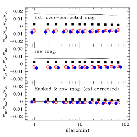
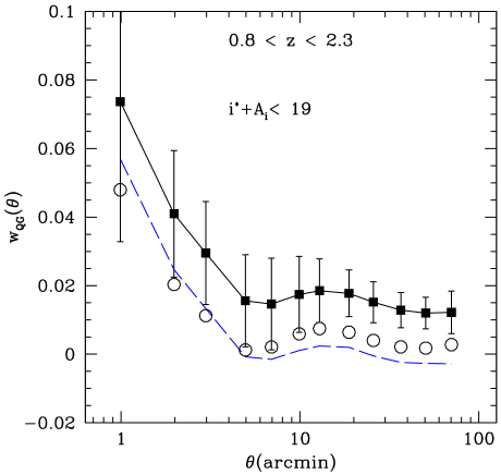
Figure 5.— Left Panel: The density variance in the extinction $<\delta^{2}_{A}>$ (closed squares), compared with galaxy-extinction cross-correlation $<\overline{\delta}_{G}~{}\delta_{A}>$ (open circles) and the QSO-extinction cross-correlation $<\overline{\delta}_{Q}~{}\delta_{A}>$ (closed circles). The continuous line shows the contamination in the galaxy-QSO cross-correlation as predicted by Eq.[8]. The top, middle and bottom panels correspond to extinction over-corrected magnitudes, raw magnitudes and results for raw magnitudes with extinction and seeing mask (which agrees well with the extinction corrected result). Right Panel: galaxy-QSO cross-correlation $w_{GQ}$ as a function of cell radius $\theta$, for objects selected with extinction over-corrected magnitudes $i^{*}<19$ (closed squares and continuous line) and raw magnitudes $i^{\prime}<19$ (open circles). The dashed line shows the prediction in Eq.[8] using $<\delta^{2}_{A}>$, $<\overline{\delta}_{G}~{}\delta_{A}>$ and $<\overline{\delta}_{Q}~{}\delta_{A}>$ cross-correlations shown in the top left panel.

3.1. Extinction and seeing mask

Following Scranton et al (2002), pixels (in 6’ resolution) with larger mean seeing or larger mean extinction than some threshold value are masked out from our analysis. The final mask is the product of this seeing and extinction mask (ie shown in Fig.3) by the sample boundary (shown in Fig.2). We have tried different thresholds following the analysis of Scranton et al (2001). As a compromise between precision and area covered, unless stated otherwise, we use 0.2 maximum extinction and seeing better than 1.8’ for $r^{\prime}<22$ and $i^{\prime}<22$. For $r^{\prime}<19$ we relax the seeing cut to 2 arc-sec to include more galaxies. For these brighter galaxies 2 arc-sec provides very good photometry for clustering analysis (see Scranton et al. 2001).

Bottom left panel in Fig.5 shows the cross-correlation results after applying the extinction mask over raw $i^{\prime}<19$ magnitudes. The resulting contamination in $w_{GQ}$ is negligible.

4. Cross-correlation measurements

For our statistical analysis, we will use moments of counts in cells, eg the variance:

$$w_{GG}(\theta)=<\delta^{2}_{G}(\theta)>$$ (9)

where $\delta_{G}\equiv n_{G}/<n>-1$ are number density fluctuations on cells of size $\theta$ (larger than the pixel map resolution) and $<n>$ is the mean number of galaxies in the cell. The average $<...>$ is over angular positions in the sky. We follow closely Gaztañaga (1994, see also Szapudi et al. 1995) and use the same software and estimators here for the SDSS. This software have been tested in different ways and the results confirmed by independent studies (eg see Szapudi & Gaztañaga 1998).

For the cross-correlation we use (see also MBM02):

$$w_{GQ}(\theta)=<\delta_{G}(\theta)\delta_{Q}(\theta)>$$ (10)

Note that this is different from the 2-point cross-correlation: $w_{2}(\theta_{12})=<\delta_{G}(\vec{\theta}_{1})\delta_{Q}(\vec{\theta}_{2})>$, where $\theta_{12}=|\vec{\theta}_{2}-\vec{\theta}_{1}|$. In our case, both cells are at the same location in the sky, and the scale dependence comes from changing the cell size. In fact, $w_{GQ}$ is just an area average over $w_{2}$, and its amplitude at scale $\theta$ is typically $20-30\%$ higher that $w_{2}$ at $\theta_{12}\simeq\theta/\sqrt{\pi}$ (see Fig.1 in Gaztañaga 1994). Also note that shot-noise cancels out for cross-correlation $w_{GQ}$, but not for $w_{GG}$ and $w_{QQ}$ where the variance needs to be shot-noise corrected (eg Gaztañaga 1994).

The reason for using the variance $w_{GQ}$ rather than the 2-point $w_{2}(\theta_{12})$ function is twofold. Firstly one expects the variance to provide better signal-to-noise ratios when the correlation signal is small, just because $w_{GQ}$ is an integrated quantity. Secondly, Ménard et al. (2002) have argued that $w_{GQ}$ provides a better estimator to improve the accuracy of the comparison with the theoretical predictions in the weak lensing regime. We have in fact performed a calculation of the $w_{2}(\theta_{12})$ cross-correlation over the same data, using the simple counts-in-cell estimator for $w_{2}(\theta_{12})$ (eg Eq.[36] in Gaztañaga 1994). The results were dominated by noise (sampling errors) and we have therefore decided to just concentrate our efforts on $w_{GQ}$.

We will also measure the galaxy-galaxy-QSO 3rd order moment:

$$w_{GGQ}(\theta)=<\delta_{G}(\theta)\delta_{G}(\theta)\delta_{Q}(\theta)>$$ (11)

and the galaxy-galaxy variance around QSOs:

$$w_{GG;Q}(\theta)=<\delta_{G}(\theta)\delta_{G}(\theta)>_{QSO}$$ (12)

The extra or excess variance is defined as (MBM02):

$$\Delta(\theta)\equiv w_{GG;Q}(\theta)-w_{GG}(\theta)$$ (13)

which turns out to be a measure of the 3-point function $w_{GGQ}(\theta)\sim\Delta(\theta)$ (Fry & Peebles 1980, MBM02).

Errors are obtained from a variation of the jackknife error scheme proposed by Scranton et al (2001, Eq.[10]). The sample is divided into $N$ separate regions on the sky, each of equal area (in our case they are cuts in RA such that the number of pixel cells is equal in each region). The analysis is performed $N$ times, each leaving a different region out. These are called (jackknife) subsamples, which we label $L=1\dots N$. The estimated statistical covariance for $w_{GQ}$ for scales $\theta_{i}$ and $\theta_{j}$ is then:

$$Covar(\theta_{i},\theta_{j}) \equiv <\Delta w_{GQ}(\theta_{i})~{}\Delta w_{GQ}(\theta_{j})>$$

$$= {N-1\over{N}}\sum_{L=1}^{N}\Delta w_{GQ}^{L}(\theta_{i})\Delta w_{GQ}^{L}(\theta_{j})$$

$$\Delta w_{GQ}^{L}(\theta_{i}) \equiv w_{GQ}^{L}(\theta_{i})-\widehat{w_{GQ}}(\theta_{i})$$ (15)

where $w_{GQ}^{L}(\theta_{i})$ is the cross-correlation measure in the $L$-th subsample ($L=1\dots N$) and $\widehat{w_{GQ}}(\theta_{i})$ is the mean value for the $N$ subsamples. The case $i=j$ gives the error variance. Note how if we increase the number of regions $N$, then jackknife subsamples are larger and each term in the sum is smaller. We have checked that the resulting covariance gives a stable answer for different $N$.

These errors has been shown to be reliable when tested against simulations in Zehavi et al (2002) and have the great advantage of being model independent. In our implementation we use $N=20$ (but we have also tried $N=10$ and $N=40$) independent regions of equal size.

4.1. Variance in the galaxy-QSO correlation

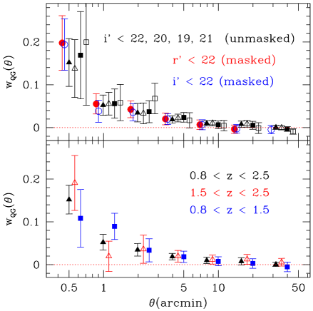
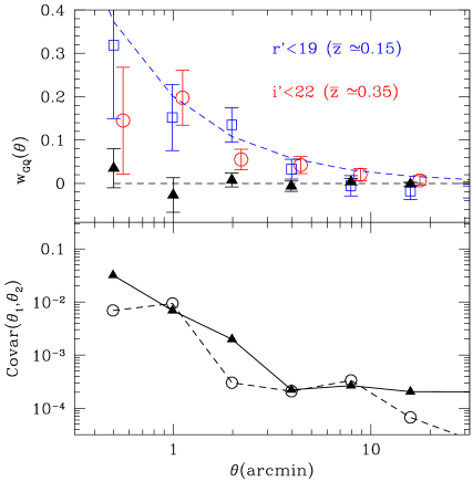
Figure 6.— Top Left panel: Galaxy-QSO cross-correlation $w_{GQ}$ (symbols with error-bars) for different galaxy samples as a function of cell radius (which is slightly shifted in each case to avoid overlaps). Closed and opened circles correspond to $i^{\prime}<22$ and $r^{\prime}<22$ with pixels masked (less than $0.2$ mag extinction and more than $2"$ seeing). Closed triangles, open triangles, closed squares and open squares, show the unmasked results for galaxies with limiting fluxes of $i^{\prime}=22,21,20,19$ respectively. Bottom Left panel: $w_{GQ}$ for $r^{\prime}=22$ galaxy sample and different redshift bins in the QSO sample: $0.8<z<1.5$ (closed squares) and $1.5<z<2.5$ (open triangles) and $0.8<z<2.5$ (closed triangles). Top Right panel: Circles and squares with error-bars show galaxy-QSO cross-correlation $w_{GQ}$ for $r^{\prime}<19$ ($\overline{z}\simeq 0.15$) and for $i^{\prime}<22$ ($\overline{z}\simeq 0.35$). Closed triangles show $w_{GQ}$ in $i^{\prime}<22$ when we randomize the galaxy counts. For comparison we also show $w_{GQ}=0.2\theta^{-0.9}$ as a dashed line. Bottom panel: Covariance $Covar(\theta_{1},\theta_{2})$ for $\theta_{1}=0.5^{\prime}$ (continuous line) and $\theta_{1}=1.0^{\prime}$ (dashed line) as a function of $\theta_{2}$.

The top-left panel of Figure 6 compares the measured values of $w_{GQ}(\theta)$ for the different magnitude bins cuts $r^{\prime}=19,20,21,22$ with unmasked pixels with the results for $r^{\prime}<22$ and $i^{\prime}<22$ with the extinction and seeing mask. All cases are roughly consistent with each other. Differences will be studied in section §5, the point here is that there is a significant signal in all bands (very similar results are find for cuts in $g^{\prime}$). Bottom left panel compares $w_{GQ}(\theta)$ when we separate the QSO in high and low redshifts.

The top-right panel of Figure 6 shows in more detail the results for $r^{\prime}<19$ ($\overline{z}\simeq 0.15$, squares) and for $i^{\prime}<22$ ($\overline{z}\simeq 0.35$, circles). The later have been shifted in angular scale (up by $\simeq 2.2$) to match the $r^{\prime}<19$ depth. Closed triangles show the $i^{\prime}<22$ results after randomizing the angular position of the galaxy counts-in-cells. This produces a distribution with identical variance, skewness and higher order moments, but which should not be correlated to the QSO sample. Thus, we expect $w_{GQ}=0$ in this case, exactly as found within the error-bars. This provides a test for our code and statistics against systematics such as boundary problems in the comparison. Also provides an indication that the errors are not underestimated.

The bottom-right panel in Figure 6 shows the covariance matrix Eq.[4] for $\theta_{1}=0.5$ (continuous line) and $\theta_{1}=1.0$ (dashed line) from the jackknife estimator with $N=40$ (values for $N=10$ are comparable but the scatter is larger). As shown in the Figure the dominant contribution comes from the diagonal terms. This is because we are using well separated bins (each cell is 4 times larger than the previous one). We neglect the off-diagonal errors in a first interpretation of the data, but we note that a stronger covariance arises from bins $\theta_{2}<\theta_{1}$ than for $\theta_{2}>\theta_{1}$, as shown in the Figure for the $\theta_{1}=1.0^{\prime}$ case.

All cases on the right panel of Figure 6 correspond to maps with extinction 0.2 and 2” seeing mask for $r^{\prime}<19$ and 1.8” seeing mask for $i^{\prime}<22$ (and $i^{\prime}_{Q}<18.8$).

Assuming no covariance, the significance of the detection (against zero correlation) for the first 5 points in top-right panel of Figure 6 is about 4-sigma in $r^{\prime}<19$ and 8-sigma in $i^{\prime}<22$.

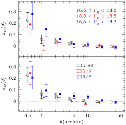
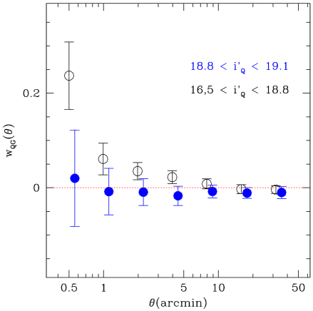
Figure 7.— Top Left panel: galaxy-QSO cross-correlation $w_{GQ}$ for $i^{\prime}<22$ galaxies with different QSO sub-samples: $16.5<i^{\prime}_{Q}<18.3$ (closed squares), $18.3<i^{\prime}_{Q}<18.8$ (closed triangles) and the combined $16.5<i^{\prime}_{Q}<18.8$ (open circles). Bottom Left panel: Comparison of the mean $w_{GQ}$ (open circles) with the values in the North (closed squares) and South (closed triangles) EDR subsamples (in all cases $i^{\prime}<22$ galaxies and $i^{\prime}_{Q}<18.8$). Right panel: Galaxy-QSO cross-correlation $w_{GQ}$ (symbols with error-bars) for $i^{\prime}<22$ galaxies with different QSO sub-samples: $16.5<i^{\prime}_{Q}<18.8$ (open circles) and $18.8<i^{\prime}_{Q}<19.1$ (closed circles).

4.2. Faint and Bright QSOs

Bottom left panel in Figure 7 shows a comparison of the results in the EDR/N and EDR/S slices with the combined sample. The agreement is good within the errors, with slightly stronger signal in EDR/S. This provides a test for different versions in the QSO selection. Runs 752/756 (which correspond to EDR/N) and 94/125 (which correspond to EDR/S) have different target selection version: v2.2a and v2.7 respectively.

Top left panel in Figure 7 shows how the masked $i^{\prime}<22$ galaxies cross-correlated with QSO subsamples cut at different $i^{\prime}_{Q}<18.8$ bands. All results agree well within the errors with stronger signal for the brighter QSO, as expected from the steeper slope of the brighter QSOs (see Fig.4).

Right panel in Figure 7 compares $w_{GQ}$ (for masked $i^{\prime}<22$ galaxies) for our nominal $16.5<i^{\prime}_{Q}<18.8$ with the faintest QSOs in EDR/QSO: $18.8<i^{\prime}_{Q}<19.1$. Note how the fainter QSO sample (closed circles) show no significant cross-correlation. This result is in fact expected (see §5 below) if the cross-correlation is truly due to weak-lensing as $\alpha\simeq 1$ for this faint sample, see Fig.4.

4.3. Comparison to galaxy-galaxy variance

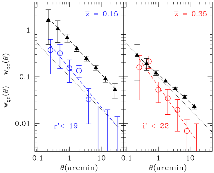
Figure 8.— Galaxy-galaxy (closed triangles) and galaxy-QSO (open circles) correlation in for bright (left panel) and faint (right panel) galaxies. Dotted-line shows $w_{GQ}=0.1\theta^{-0.7}$ for comparison, dashed-lines are power-law fits to the data. Galaxy-galaxy correlations have been shifted slightly to the left of the corresponding galaxy-QSO values to avoid intersection of the error-bars.

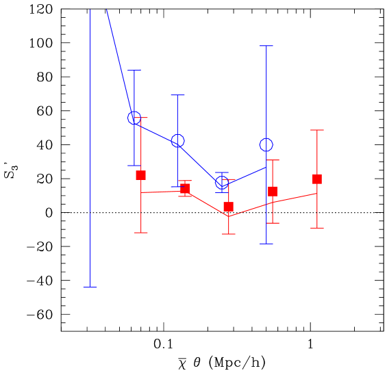
Figure 9.— Pseudo-Skewness Eq.[18] as a function of $\theta$. Square (circles) correspond to $\overline{z}\simeq 0.35$ ($\overline{z}\simeq 0.15$). Continuous lines in each case correspond to the excess skewness Eq.[19].

Fig.8 summarizes the main observational results in this paper. We compare $w_{GQ}(\theta)$ (open circles) and $w_{GG}(\theta)$ (closed triangles) for bright $i^{\prime}_{Q}<18.8$ QSOs with faint ($r^{\prime}<19$) and bright $i^{\prime}<22$ galaxies samples. The dotted line shows (for comparison) the power-law $w_{GQ}=0.1\theta^{-0.7}$. The $i^{\prime}<22$ case is also shown as closed circles in the top-left panel of Fig.6.

All data is well fitted to power-laws taking into account the errors (and neglecting the covariance). We find:

$$\begin{array}[]{ll}\beta_{GG}\equiv{d\log{w_{GG}}\over{d\log(\theta)}}=&\left\{\begin{array}[]{ll}-0.72\pm 0.02~{}~{}~{}~{}\overline{z}\simeq 0.15\\ -0.60\pm 0.03~{}~{}~{}~{}\overline{z}\simeq 0.35\end{array}\right.\end{array}$$ (16)

$$\begin{array}[]{ll}\beta_{GQ}\equiv{d\log{w_{GQ}}\over{d\log(\theta)}}=&\left\{\begin{array}[]{ll}-0.83\pm 0.17~{}~{}~{}~{}\overline{z}\simeq 0.15\\ -0.96\pm 0.13~{}~{}~{}~{}\overline{z}\simeq 0.35\end{array}\right.\end{array}$$ (17)

4.4. The Skewness

Fig.9 shows the pseudo-skewness (symbols with error-bars):

$$S^{\prime}_{3}(\theta)\equiv{w_{GGQ}(\theta)\over{w_{GQ}^{2}(\theta)}}$$ (18)

and the normalized excess skewness (continuous lines):

$$S^{\Delta}_{3}(\theta)\equiv{\Delta(\theta)\over{w_{GQ}^{2}(\theta)}}={w_{GG;Q}(\theta)-w_{GG}(\theta)\over{w_{GQ}^{2}(\theta)}}$$ (19)

where $w_{GG;Q}$ is the galaxy variance around QSOs. It is expected that both quantities, $S^{\prime}_{3}$ and $S^{\Delta}_{3}$, should roughly agree on large scales. In fact, when shot-noise can be neglected $S^{\Delta}_{3}=S^{\prime}_{3}-1$ (see MBM02). Within the errors this relation is in good agreement with Fig.9.

A fit of a constant skewness in Fig.9 gives:

$$\begin{array}[]{ll}S_{3}^{\prime}~{}=&\left\{\begin{array}[]{ll}20.6\pm 5.7~{}~{}~{}~{}{\overline{z}}\simeq 0.15\\ 13.6\pm 4.3~{}~{}~{}~{}{\overline{z}}\simeq 0.35\end{array}\right.\end{array}$$ (20)

In Fig.9 we have used the masked mapped with $0.2$ reddening and $2"$ seeing. Results for other choices of the mask parameters are similar.

5. Comparison with predictions

Consider the case of power-law correlations: $\xi(r)=\left({r_{0}\over{r}}\right)^{\gamma}$ or $P(k)\sim k^{n}$, with $\gamma=n+3$. In current models of structure formation $n$ or $\gamma$ vary only smoothly with scale, so this should be a good approximation if we limit our study to a small range of scales. We will normalized the amplitude as:

$$\overline{\xi}(R)=\sigma_{0.2}^{2}\left({0.2Mpc/h\over{R}}\right)^{\gamma}$$ (21)

where $\sigma^{2}_{0.2}$ refers to the non-linear amplitude of mass fluctuations on scales of $0.2Mpc/h$, which correspond to $\sim 1^{\prime}$ in the sky.

Galaxies might not be fair traces of the underlaying mass distribution. This is in fact one of the main motivations to use weak lensing as a tool to study large scale structure. In the Appendix we give a prescription to parameterize the possible bias that relates galaxies and matter distributions. For a power-law correlation, this parameterization allows for a shift $b_{0.2}$ in the amplitude and also a shift $\gamma_{b}$ in the slope of the galaxy correlation with respect to that of the matter distribution.

5.1. Projection and lens magnification

To simplify notation, and without lost of generality, we will give all expression for a flat universe, $\Omega_{m}+\Omega_{\Lambda}=1$, where the comoving angular distance $r(\chi)$ equals the radial comoving distance $\chi$ (see Bernardeau, Van Waerbeke & Mellier 1997, Moessner & Jain 1998, for the more general case). Also, by default, assume $\Omega_{m}=0.3$, in agreement with current observations (see §6).

The $\chi$ distance is given in terms of the redshift $z$ by:

$$d\chi={dz\over{E(z)}}~{}~{}~{};~{}~{}~{}E(z)={H_{0}\over{c}}\sqrt{1-\Omega_{m}+(1+z)^{3}\Omega_{m}}$$ (22)

which can be used to map $\chi=\chi(z)$ and $z=z(\chi)$. For $\overline{z}\simeq 0.15$ we find a mean $\chi\simeq 430$ Mpc/h, while $\overline{z}\simeq 0.35$ we have $\chi\simeq 960$ Mpc/h.

The projected galaxy fluctuation is:

$$\delta_{G}(\theta)=\int_{0}^{\chi_{H}}~{}d\chi~{}W_{G}(\chi)~{}\delta_{G}(\chi,\theta)$$ (23)

where $\chi_{H}$ is the distance to the horizon and $\theta$ refers to either the angular position in the sky or the radius of a circular cell in the sky. In the later case, which is the one we will study, $\delta$ is smoothed over a cell or radius $\theta$ (a cone in the sky). The galaxy selection function $W_{G}(\chi)$ corresponds to the probability of including a galaxy in the survey and is normalized to unity:

$$\int_{0}^{\chi_{H}}~{}d\chi~{}W_{G}(\chi)=\int_{0}^{z_{H}}~{}dz~{}n_{G}(z)=1$$ (24)

where $n(z)$ is the normalized redshift distribution.

On the other hand, fluctuations in the flux limited QSO induced by weak lensing magnification, $\delta_{\mu}$, can be expressed in terms of the weak lensing convergence ${\cal K}$:

$$\delta_{\mu}(\theta)=2~{}(\alpha-1)~{}{\cal K}(\theta)$$ (25)

where $\alpha$ is the slope of the QSO number counts:

$$N(>i^{\prime}_{Q})\sim 10^{0.4~{}\alpha~{}i^{\prime}_{Q}}$$ (26)

In our sample we find a least square fit of $\alpha\simeq 1.88\pm 0.03$ in the range $18.4<i^{\prime}_{Q}<18.9$ (shown as continuous line in Fig.4). The convergence is given by a projection over the radial matter fluctuation $\delta(\chi,\theta)$, that acts as a lens. This projection is an integral over the lensing magnification efficiency, ${\cal E}(\chi)$, a geometrical factor $\simeq{{\chi_{Q}-\chi}\over{\chi_{Q}}}$ that depends on the QSO $\chi_{Q}$ radial distribution and $\Omega_{m}$. We express this projection as:

$$\delta_{\mu}(\theta)=\int_{0}^{\chi_{H}}~{}d\chi~{}{\cal E}(\chi)~{}\delta(\chi,\theta)$$ (27)

where

$${\cal E}(\chi)=2(\alpha-1){3H_{0}^{2}\Omega_{m}\over{2~{}c^{2}}}(1+z)\chi\int_{\chi}^{\chi_{H}}d\chi^{\prime}{{\chi^{\prime}-\chi}\over{\chi^{\prime}}}~{}W_{Q}(\chi^{\prime})$$ (28)

and $W_{Q}(\chi)$ is given by the normalized probability to include a QSO in our sample:

$$\int_{0}^{\chi_{H}}~{}d\chi~{}W_{Q}(\chi)=\int_{0}^{z_{H}}~{}dz~{}n_{Q}(z)=1$$ (29)

As noted in Bernardeau, Van Waerbeke & Mellier (1997), the crucial difference between galaxy projection in Eq.[23] and lensing magnification in Eq.[27] is that ${\cal E}$ is not normalized to unity. Thus, besides the projection effect, which can be modeled as an stochastic selection function, we have an overall re-scaling of fluctuation amplitudes (this has been used in Gaztañaga & Bernardeau 1998 to produce simple non-linear weak-lensing simulations). Figure 10 compares ${\cal E}(z)/E(z)$ with $n_{G}(z)$ and $n_{Q}(z)$ for the QSO and galaxy samples in our analysis. For QSOs the redshift distribution is the one measured in the EDR/QSO $16.5<i_{Q}<18.8$ sample, while for galaxies we show the predictions in Dodelson et al. (2001).

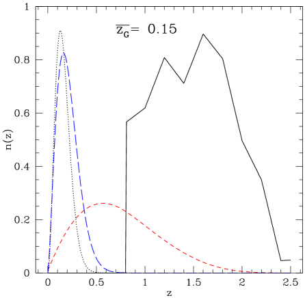
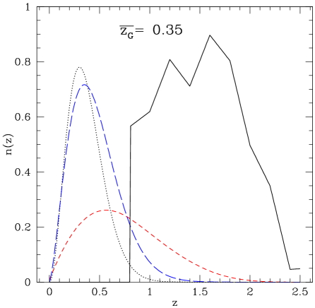
Figure 10.— The dotted line shows the predicted galaxy redshift distribution $n_{G}(z)$ (divided by 3 to be on scale) for $\overline{z}=0.35$ (right panel), which corresponds to $r^{\prime}<22$ (and also $i^{\prime}<22$) and for $\overline{z}=0.15$ (left panel), which corresponds to $r^{\prime}<19$. The continuous line shows the normalized QSO redshift distribution $n_{Q}(z)$ as measured in EDR/QSO. Short-dashed line is the lensing magnification efficiency ${\cal E}(z)/E(z)$ for the shown $n_{Q}(z)$. The long-dashed line corresponds to $\sqrt{n_{G}(z)~{}{\cal E}(z)/E(z)}$ which roughly represents the efficiency of galaxy-QSO cross-correlation.

5.2. Mass-mass and galaxy-galaxy correlations

Using Eq.[21] and within the small angle approximation( eg see §7.2.1 in Bernardeau et al. 2002), the variance of the projected mass fluctuations can be expressed as:

$$w(\theta)\equiv<\delta^{2}(\theta)>=\sigma_{0.2}^{2}~{}A~{}\theta^{1-\gamma}$$ (30)

where

$$A = A(\gamma)=B(\gamma)~{}T_{\gamma}~{}\overline{W^{2}_{G}}$$ (31)

$$B(\gamma) \equiv {(3-\gamma)~{}(4-\gamma)~{}(6-\gamma)~{}\Gamma(\gamma/2-1/2)\Gamma(1/2)\over{5^{\gamma}~{}2^{3-\gamma}~{}9~{}\Gamma(\gamma/2)}}$$

$T_{\gamma}$ is a geometrical factor of order unity ($T_{\gamma}\simeq 0.7-0.8$) that comes from the area average over the 2-point function:

$$T_{\gamma}\equiv{4\over{\pi(5-\gamma)}}\int_{0}^{1}x~{}dx\int_{0}^{2\pi}d\phi\left(1+x^{2}-2x\cos{\phi}\right)^{{1-\gamma}\over{2}},$$ (32)

and $\overline{W^{2}_{G}}$ is given by the radial galaxy selection:

$$\overline{W^{2}_{G}}\equiv\int_{0}^{\chi_{H}}~{}d\chi~{}W_{G}^{2}(\chi)~{}\chi^{1-\gamma}D^{2}(z)$$ (33)

where $D(z)$ accounts for the redshift evolution of the correlation function: eg in the linear regime $D(z)$ is the linear growth factor, in the stable clustering regime $D^{2}(z)=(1+z)^{-3}$.

For the galaxy-galaxy variance we assume the bias in Eq.[A4], which allows for a shift $b_{0.2}$ in the amplitude and also a shift $\gamma_{b}$ in the slope of the galaxy correlation with respect to that of the matter distribution. Thus, we have:

$$w_{GG}(\theta)\equiv<\delta^{2}_{G}(\theta)>=b_{0.2}^{2}~{}\sigma_{0.2}^{2}~{}A_{GG}~{}\theta^{1-\gamma-2\gamma_{b}}$$ (34)

where $A_{GG}$ is the same as $A$ in Eq.[31] for the new slope: $A_{GG}=A(\gamma+2\gamma_{b})$.

5.3. QSO-QSO and galaxy-QSO correlations

We next want to estimate the galaxy-QSO cross-correlation. We express the angular QSO fluctuations as:

$$\delta_{Q}(\theta)=\delta_{Q}^{I}(\theta)+\delta_{\mu}(\theta)$$ (35)

where $\delta_{Q}^{I}(\theta)$ stands for the intrinsic fluctuations while $\delta_{\mu}(\theta)$ are fluctuations induced by magnification bias. Neglecting the QSO (source) and matter (lens) cross-correlation (which is negligible given the large radial separations), the observed QSO variance has two contributions:

$$w_{QQ}(\theta)\equiv<\delta_{Q}(\theta)~{}\delta_{Q}(\theta)>=w^{I}_{QQ}(\theta)+w_{\mu\mu}(\theta)$$ (36)

where:

$$w_{\mu\mu}(\theta)\equiv<\delta^{2}_{\mu}(\theta)>=\sigma_{0.2}^{2}~{}A_{QQ}~{}\theta^{1-\gamma}$$ (37)

with:

$$A_{QQ} = B(\gamma)~{}T_{\gamma}~{}\overline{{\cal E}^{2}}$$ (38)

$$\overline{{\cal E}^{2}} \equiv \int_{0}^{\chi_{H}}~{}d\chi~{}{\cal E}^{2}(\chi)~{}\chi^{1-\gamma}D^{2}(z).$$

The above expressions can be used, for a known magnification, to separate the intrinsic from the apparent QSO clustering.

The QSO and galaxy populations are well separated in radial distances so that we can neglect the intrinsic cross-correlation $<\delta_{G}(\theta)~{}\delta_{Q}^{I}(\theta)>$. We then have:

$$w_{GQ}(\theta)\equiv<\delta_{G}(\theta)~{}\delta_{Q}(\theta)>\simeq<\delta_{G}(\theta)~{}\delta_{\mu}(\theta)>$$ (39)

so that using Eq.[27] and assuming Eq.[A4] we find:

$$w_{GQ}(\theta)=b_{0.2}~{}\sigma_{0.2}^{2}~{}A_{GQ}~{}\theta^{1-\gamma-\gamma_{b}},$$ (40)

with:

$$A_{GQ} = B(\gamma+\gamma_{b})~{}T_{\gamma+\gamma_{b}}~{}\overline{W_{G}{\cal E}}$$ (41)

$$\overline{W_{G}{\cal E}} \equiv \int_{0}^{\chi_{H}}~{}d\chi~{}W_{G}(\chi)~{}{\cal E}(\chi)~{}\chi^{1-\gamma-\gamma_{b}}D^{2}(z)$$

5.4. Measure of bias and matter fluctuations

The combination galaxy-galaxy and galaxy-QSO cross-correlation will allow us to break the intrinsic degeneracy between biasing and matter fluctuations, eg between $b_{0.2}$ and $\sigma_{0.2}$ as measured by galaxy surveys alone. Here, we propose to measure the four parameters that characterize bias and matter fluctuations in a narrow range of scales (the power-law approximation). These parameters are $\sigma_{0.2}^{2}$ and $\gamma$ for the variance in non-linear mass fluctuations (eg Eq.[21]) and $b_{0.2}$, $\gamma_{b}$ for the bias function as described in the Appendix, eg Eq.[A4].

We can estimate these four parameters, $\sigma_{0.2}$, $b_{0.2}$, $\gamma$ and $\gamma_{b}$, from the angular observations of galaxy-QSO correlations in the following way. We first take the measured logarithmic slopes of $w_{GG}$ and $w_{GQ}$ in Eq.[16]-[17] from a fit to the data in Fig.8. These slopes and the used to find the intrinsic matter slope $\gamma$ and bias scale dependence $\gamma_{b}$:

$$\gamma = 1+\beta_{GG}-2\beta_{GQ}$$

$$\gamma_{b} = \beta_{GQ}-\beta_{GG}$$ (42)

We can then obtained $b_{0.2}$ and $\sigma_{0.2}$ as:

$$b_{0.2} = {{w_{GG}(\theta)}\over{w_{GQ}(\theta)}}~{}{A_{GQ}\over{A_{GG}}}~{}\theta^{\gamma_{b}}$$

$$\sigma^{2}_{0.2} = {{w_{GQ}^{2}(\theta)}\over{w_{GG}(\theta)}}~{}{A_{GG}\over{A^{2}_{GQ}}}~{}\theta^{\gamma-1}$$ (43)

If the power-law model is a good approximation these values should not be a strong function of scale. This will provide a consistency test for our power-law approximation.

The above reconstruction scheme has been tested against mock angular simulations in Gaztañaga (1995). This method can be generalized to extract the shape $\overline{\xi}(R)$ from $w_{GG}(\theta)$ in the quasi-scale invariance approximation by performing local inversions around $R\simeq\theta\chi$, where $\chi$ is the mean depth of the sample (see Gaztañaga 1995 for details). We have also verified the validity of such approximations over the weak lensing simulations presented in Gaztañaga & Bernardeau (1998).

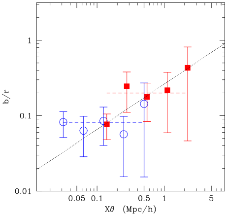
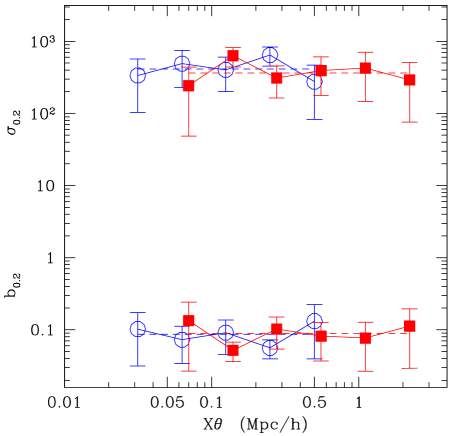
Figure 11.— In both panels: open circles correspond to $r^{\prime}<19$ ($\overline{z}=0.15$) and closed squares to $i^{\prime}<22$ ($\overline{z}=0.35$). Left Panel: Values of $b/r$ de-projected from the ratio $w_{GG}/w_{GQ}$ assuming a constant, but stochastic, bias. Dashed lines are the best fit constant value of $b/r$ for each galaxy sample. The dotted line gives the best fit linear relation for both samples. Right Panel: Values of $b_{0.2}$ and $\sigma_{0.2}$ de-projected using Eq.[43], as a function of scale.

5.5. Scale dependence bias

Left panel of Fig.11 shows $b/r$ defined in Eq.[A13] and de-projected from the data at each point as

$${b\over{r}}={w_{GG}\over{w_{GQ}}}{A_{GQ}\over{A_{GG}}},$$ (44)

ie assuming that $b/r$ is scale independent (ie $\gamma_{b}=0$). Each point is shown at scale corresponding to the mean depth in the sample $\chi\theta$. The resulting values of $b/r$ show a tendency to increase with scale, which means that $\gamma_{b}=0$ is not such a good approximation. But note that this trend is not very significant given the large errorbars: a constant value of $b/r$ is only ruled out with a 3-sigma significance.

Right panel of Fig.11 shows the recovered values of $\sigma_{0.2}$ and $b_{0.2}$ as a function of scale given the prescription in Eq.[43]. The recovered values are quite flat, in good agreement with the assumption that the correlation functions can be approximated locally by power-laws (eg Eq.[34]).

5.6. Results for $\sigma_{0.2}$, $b_{0.2}$, $\gamma$ and $\gamma_{b}$

From Eq.[16]-[17] and Eq.[42]:

$$\begin{array}[]{ll}\gamma~{}=&\left\{\begin{array}[]{ll}1.94\pm 0.34~{}~{}~{}~{}\overline{z}\simeq 0.15\\ 2.33\pm 0.26~{}~{}~{}~{}\overline{z}\simeq 0.35\end{array}\right.\end{array}$$ (45)

$$\begin{array}[]{ll}\gamma_{b}~{}=&\left\{\begin{array}[]{ll}-0.11\pm 0.17~{}~{}~{}~{}\overline{z}\simeq 0.15\\ -0.36\pm 0.13~{}~{}~{}~{}\overline{z}\simeq 0.35\end{array}\right.\end{array}$$ (46)

While the mean values from right panel of Fig.11 are:

$$\begin{array}[]{ll}b_{0.2}~{}=&\left\{\begin{array}[]{ll}0.09\pm 0.02~{}~{}~{}~{}\overline{z}\simeq 0.15\\ 0.09\pm 0.02~{}~{}~{}~{}\overline{z}\simeq 0.35\end{array}\right.\end{array}$$ (47)

$$\begin{array}[]{ll}\sigma_{0.2}~{}=&\left\{\begin{array}[]{ll}412\pm 97~{}~{}~{}~{}\overline{z}\simeq 0.15\\ 364\pm 86~{}~{}~{}~{}\overline{z}\simeq 0.35\end{array}\right.\end{array}$$ (48)

These values assume that clustering is fixed in comoving coordinates. Values for other clustering evolution, ie $\epsilon\neq 0$, can be obtained using in Eq.[33]:

$$D^{2}(z)\simeq(1+z)^{-(3+\epsilon)}$$ (49)

If we require the underlaying ($z=0$) $\sigma_{0.2}$ to be the same in both samples we find:

$$\epsilon\simeq 0.8\pm 1.3$$ (50)

which roughly agrees with stable clustering, but has a large error.

6. Discussion

As we will show in some detailed here, the values we have recovered for $\sigma_{0.2}$, $b_{0.2}$, $\gamma$ and $\gamma_{b}$ appear in contradiction with currently popular expectations. We should therefore discuss first the two more important systematics in our analysis: error-bar estimation (section §6.1) and extinction (§6.2).

In §6.3 we give a brief account of what are the currently popular expectations for the above observables. In §6.4 we will show how the results we find in this paper seem to contradict the expectations. A possible solution for this contradiction is hinted in §6.5 and §6.6 as we consider clustering evolution in shape and amplitude. In subsection 6.7 we discuss how our interpretation changes with $\Omega_{m}$ and find that our proposed solution can also explained the low value of the measured skewness. Finally in §6.8, we compare our results with other estimates.

6.1. Unrealistic or correlated error-bars?

We have sliced the data, as displaced in Fig.1, in $N=10-40$ RA bins (horizontal direction in the Figure). Because of the mask, this results in subsamples with different shapes and holes, which increases the sample-to-sample scatter in the jackknife error estimation Eq[4]. Thus we believe that this approach is conservative and slightly overestimates all the jackknife errorbars presented in the above section. We have tested this idea with the APM (Maddox et al. 1990) pixel maps.

We compare the jackknife error over a given slice out of the APM map against the scatter from different slices (the APM can fit over 20 EDR slices). The jackknife error is comparable to the zone to zone scatter on scales larger than a few arc-minutes (where the mean density of galaxies in a cell is larger than unity), but is about a factor of 3 larger than the zone to zone errors on the smallest scales (dominated by shot-noise fluctuations). We do not attempt to correct for this here, but rather take the conservative approach of using the jackknife errors. This means that in principle the significance of the analysis presented below can be improved with a more sophisticated treatment of errors (eg see Colombi, Szapudi & Szalay 1998).

There is also an overall shift in the mean amplitude of the zone to zone correlations (variance or skewness), due to large scale (sample size) density fluctuations, which is not taken into account by the jackknife error. The amplitude of this effect is comparable to the jackknife error on 20’ scales. This is similar to an overall calibration error as indeed corresponds to the uncertainty in the value of the mean density over the whole map (eg see Hui & Gaztañaga 1999). Our error analysis hardly changes if we take this into account as we are mostly dominated by the (relatively large) scatter from shot-noise and small scale fluctuations.

Other than this, the covariance shown in bottom-right panel of Figure 6 seems to be dominated by the diagonal terms and we have neglected it.

6.2. Variable obscuration from the Galaxy

Could our result be caused by small scale variations from obscuration in our galaxy? In §3 we have shown that large scale extinction is not affecting our results. There is a small but significant anti-correlation of the SDSS/EDR galaxy and QSO maps with Schlegel et al. (1998) which induces an artificial galaxy-QSO cross-correlation. We have shown how this effect disappears when using an extinction mask. But Schlegel et al. (1998) maps have a FWHM of $\theta=6^{\prime}$, while we measure correlations below $\theta=1^{\prime}$. Could our cross-correlation be caused by extinction at smaller scales? The spectrum of extinction fluctuations as measured by Schlegel et al. (1998), $P(k)\propto k^{-2.5}$ at scales from $\simeq 6$ arc-min to $\simeq 30$ degrees. , indicates that the amplitude of density fluctuations induced by absorption $<\delta^{2}_{A}>\propto\theta^{+0.5}$ grows slowly with scales. Thus extinction produces larger galaxy-QSO artifacts on larger scales.

Extrapolating this spectrum to smaller scales should produce smaller contributions than the ones we have already estimated in §3. In summary, the detected galaxy-QSO cross-correlation have therefore the wrong amplitude and the wrong shape to be explained by galactic extinction.

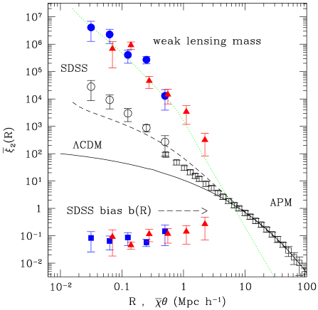
Figure 12.— Left panel: Comparison of the linear (continuous line) and non-linear (open squares) variance in the $\Lambda$CDM simulations ($\overline{\xi}^{\Lambda CDM}$) with that in APM galaxies ($\overline{\xi}^{A}PM$, squares with error-bars), from Fig.11 in Gaztañaga (1995). Dashed lines shows the non-linear fitting formulae of Smith et al. (2002). The inset shows the bias function $b(R)\equiv\sqrt{{\overline{\xi}^{A}PM\over{\overline{\xi}^{\Lambda CDM}}}}$ for the non-linear (closed squares with errorbars) and linear $\Lambda$CDM (continuous line) cases. Right panel: Comparison of the linear (continuous line) and non-linear (dashed line) variance in the $\Lambda$CDM model with that from the $b_{J}<20$ APM galaxies (open squares with error-bars) and $r^{\prime}<19$ SDSS galaxies ( open circles with error-bars). Upper closed circles and triangles show the non-linear variance reconstructed from the galaxy-QSO correlation in the EDR/SDSS at $\overline{z}\simeq 0.15$ and $\overline{z}\simeq 0.35$ (scaled to $z=0$ under stable clustering). Lower closed figures show the corresponding results for the bias function $b(R)$. The dotted line shows the non-linear mass variance prediction for a steep $n_{eff}\simeq 0.97$ initial spectrum.

6.3. The standard $\Lambda$CDM picture

In the non-linear regime dark-matter ($\Lambda CDM$) numerical simulations typically find that on cluster scales ($r\simeq 0.1$ Mpc/h) the non-linear variance of density fluctuations is $\overline{\xi}_{NL}\simeq 10^{2}\overline{\xi}_{L}$, where $\overline{\xi}_{L}$ stands for the linear value (compare continuous line with short-dashed line in left panel of Fig.12). Moreover $\overline{\xi}_{NL}\sim R^{-1}$ ( $\sim R^{-3/2}$ at the non-linear transition) which is typically steeper than the linear values $\overline{\xi}_{L}\sim R^{-1/2}$ ( $\sim R^{-1}$ at the non-linear transition). This behavior is reproduced by the non-linear fitting formulaes (eg Peacock & Dodds 1996) and have been extensively used in weak-lensing predictions (eg Bartelmann & Schneider 2001, Benitez et al. 2001). For galaxies, predictions vary from model to model but one can typically find that on non-linear scales (1 to 10 Mpc/h) $\overline{\xi}_{G}\simeq\overline{\xi}_{L}$ for blue (Late-type) galaxies and up to $\overline{\xi}_{G}\simeq 10\overline{\xi}_{NL}$ for the red (Early-type) population. This gives a range $b\simeq\sqrt{\overline{\xi}_{G}/\overline{\xi}_{NL}}\simeq 0.1$ and $b\simeq 3$. This is also in rough agreement with the estimations in galaxy surveys. We will call this the standard $\Lambda$CDM picture for non-linear galaxy and mass evolution (see Cooray & Sheth 2002 for an excellent review on all the above ideas).

In terms of the variance most of these features can be summarized in the left panel of Figure 12, which is a expanded version of Fig.11 in Gaztañaga (1995). Note how APM galaxies seem to be anti-bias on small scales with respect the $\Lambda$CDM model, something that seems to be compatible with different models of galaxy formation (eg Jenkins et al. 1998, Seljak 2000, Scoccimarro et al. 2001a, Sheth et al. 2001 and references therein).

6.4. Weak lensing magnification

If we take the detected galaxy-QSO cross-correlation signal as being purely due to weak lensing magnification, we find important challenges for the above picture, even in the orders of magnitude involved. These are summarized in right panel of Fig.12, which shows the recovered mass variance as a function of scale. We find $b\simeq 0.1$ (which seems to agree with the above blue galaxy model above) but note that $\overline{\xi}_{NL}\simeq 10^{4}\overline{\xi}_{L}$ (ie compared upper closed figures, $\overline{\xi}_{NL}$, with dashed line, $\overline{\xi}_{L}$) which is much larger than expected in the standard $\Lambda$CDM picture above.

We also find some evolutionary trends. First of all, from Eq.[45] we find $\overline{\xi}_{NL}\sim R^{-2}$ which is steeper (3 sigma significance) than in the standard $\Lambda$CDM picture (slope of the dashed line in right panel of Fig.12). At higher redshifts ($\overline{z}\sim 0.35$) the slope seems slightly steeper $\overline{\xi}_{NL}\sim R^{-2.3}$, as expected if we assume that on average there are lower mass halos at higher redshifts, and therefore steeper profiles (see Navarro, Frenk & White 1996). Obviously, the slope of the galaxy $\overline{\xi}_{G}$ distribution is the same as in the standard $\Lambda$CDM picture (as these are direct observations that we also reproduce in our analysis).

The measured values of the amplitude today $\sigma_{0.2}\simeq 400$ is about $100$ times larger that expected in the standard $\Lambda$CDM picture, although the discrepancy factor depends on the particular cosmology. The significance of this result is over 4-sigma.

The biasing amplitude $b$ at $0.2$ Mpc/h remains constant $b\simeq 0.1$ with redshift. The null hypothesis of $b=1$ is ruled out at a large significance. The slope $\gamma_{b}$ (ie from Eq.[46]) seems to become more negative at $\overline{z}\sim 0.35$ (only 1-sigma effect), which partially masks the steepening of the density profiles as we increase the redshift.

On weakly non-linear scales, the shape of the galaxy 3-point function and bispectrum can be used to determine $b$ with independence of the underlaying spectrum. This was first proposed by Frieman & Gaztañaga (1994) and Fry (1994), following the ideas in Fry & Gaztañaga (1993). Recent measurements ( Frieman & Gaztañaga 1999, Scoccimarro et al. 2001b, Verde et. al 2002) find $b\simeq 1$ at scales $>10$ Mpc/h. In fact this value is not in contradiction with the values above as the bias seems to increase with scale, which extrapolates well to $b\simeq 1$ at $\simeq 10$ Mpc/h.

Our recovered valued do not assume any model for the primordial spectrum or its subsequent evolution, but assumed a flat geometry with $\Omega_{m}=0.3$. This affects both the projection and the amplitude of the lensing magnification. The geometry enters in both the lensing and the galaxy projections and should therefore cancel out to some extend for $b$, but not quite for $\overline{\xi}_{NL}$ which is estimated from ratio $w^{2}_{GQ}/w_{GG}$. Thus we expect our estimations of $b$ to scale with $\sim{\Omega_{m}\over{0.3}}$ and $\overline{\xi}_{NL}$ as $\sim({0.3\over{\Omega_{m}}})^{1.5}$ (see Bernardeau et al. 1997). Thus if $\Omega_{m}\simeq 1$ this would produce $b\simeq 0.3$ and $\sigma_{0.2}\simeq 158$. These values are closer to the standard $\Lambda$CDM picture above but still uncomfortably far from it. Moreover they represent an inconsistency in the value of $\Omega_{m}$.

If the standard $\Lambda$CDM picture fails on these small scales, is there any possible alternative?

6.5. Stable clustering

The amplitude of $\overline{\xi}_{NL}$ at $0.2$ Mpc/h follows the stable clustering regime (structures are decoupled from the Hubble expansion): $\overline{\xi}\sim(1+z)^{-(3+\epsilon)}$, with $\epsilon\simeq 0$, indicating that indeed clustering could be dominated by the halo profile ($1h$) rather than by the relative distribution of halo pairs ($2h$ term in Eq.[86] of Cooray & Sheth 2002). The fact that the recovered amplitudes at redshifts $\overline{z}_{1}\simeq 0.15$ and $\overline{z}_{2}\simeq 0.35$ follow:

$${\overline{\xi}(\overline{z}_{1})\over{\overline{\xi}(\overline{z}_{2})}}\simeq\left({1+\overline{z}_{1}\over{1+\overline{z}_{2}}}\right)^{-3}\simeq 1.6$$ (51)

does not involved any parameter fitting and is non trivial given that the raw observed correlation at different redshifts are quite different (eg see Fig.[8]). In other words, there is no reason to expect any systematic effect to mimic this redshift dependence. Note that both in the linear regime $\overline{\xi}_{L}\simeq D^{2}\overline{\xi}_{0}$ and in the strongly non-linear regime, this ratio should be independent of the amplitude $\overline{\xi}_{0}$ of the primordial spectrum. The fact that is good agreement with stable clustering on scales where clusters have collapsed is not surprising. Unfortunately the error we find for $\epsilon$ in Eq.[50] is too large to draw more significant conclusions.

There is another aspect to stable clustering, which is related to the scale dependence of the correlations. Peebles (1980) have shown that in the stable clustering for a power-law initial spectrum $\overline{\xi}_{L}\sim R^{-(n+3)}$ (where $n$ is the index of the linear spectrum $P(k)\sim k^{n}$), the non-linear slope $\overline{\xi}_{NL}\sim R^{-\gamma}$ is:

$$\gamma={3(n+3)\over{5+n}}$$ (52)

In the $\Lambda$CDM models $n\simeq-1.5$ on non-linear scales so that one would expect $\gamma\simeq 1.3$. Smith et al. find that N-body simulations in fact fall a bit short of this prediction, with $\gamma\simeq 1.0$. For other values of $n$ they find that $\gamma$ increases with the steepness roughly as predicted by the stable clustering, but the measure $\gamma$ always falls a bit below the stable clustering prediction in Eq.[52] (see Fig. 9 in Smith et al. 2002). It should be noted that the agreement seems to improve for steep slopes: ie at $n=0$, Smith et al. (2002) find $\gamma\simeq 1.7$ while Eq.[52] gives $\gamma=1.8$. Also note that Eq.[52] might be valid for stronger non-linearities (or smaller scales) than tested in the Smith et al (2002) simulations.

Thus, the value we find from the galaxy-QSO data, $\gamma\simeq 2$ in Eq.45], indicates a spectrum $n\simeq 1$ in Eq.[52]. This value is very different from the standard $\Lambda$CDM picture. But we will now show that in fact, for such steep initial spectrum normalized to $\sigma_{8}\simeq 1$, one expects the non-linear amplitude to be $\sigma_{0.2}\simeq 400$, just as found in the our interpretation of the galaxy-QSO correlations.

6.6. Non-linearities and halo model

One of the possible origins of the discrepancy that we find for the measured value of $\sigma_{0.2}$ as compared with the standard $\Lambda$CDM picture is the modeling of the non-linear variance $\overline{\xi}_{NL}$. Based in the stable clustering ideas, Hamilton et al (1991) proposed that the non-linear variance should be a fixed universal function $f_{NL}$ of the linear variance once we identify the adequate mapping of linear to non-linear scales: $\overline{\xi}_{NL}\simeq f_{NL}(\overline{\xi}_{L})$. Under stable clustering, the cosmic evolution of $\overline{\xi}_{NL}$ with the scale factor $a$ is $\overline{\xi}_{NL}\sim a^{3}$ while $\overline{\xi}_{L}\sim a^{2}$, which implies that $\overline{\xi}_{NL}\simeq\overline{\xi}_{L}^{3/2}$. These transformations were generalized to the power spectrum and to models with $\Omega\neq 1$ by Peacock & Dodds (1994, 1996) and Jain, Mo & White (1995) to provide phenomenological fitting formulaes for non-linear clustering which have since been widely used. The range of validity and the accuracy of these initial ansatze was limited and, when looked in detail, there appears to be a fundamental problem in getting a universal fit that works for scale dependent models (see Baugh & Gaztañaga 1996, Smith et al. 2002).

A more recent realization of this idea involves the dark matter halo approach (see Cooray & Sheth 2002 for a review) which assumes that the density field can be modeled by a distribution of clumps of matter (the halos) with some density profile. The large-scale clustering of the mass in the linear (and weakly non-linear) regime is given by that of the correlation between halos, which should trace the linear (and weakly non-linear) perturbation theory predictions, while the small-scale clustering of the mass arises from a convolution of the halo density profile with itself. Thus, in this model the results from weak-lensing magnification in right panel of Fig.12 mostly traces the halo profiles.

Smith et al. (2002) present new versions of the universal non-linear fitting formulae $f_{NL}$ that incorporate these new ideas. The new formulae seems to perform quite well against the Virgo N-body simulations. For the $\Lambda$CDM model, the comparison involves scales up to $k\simeq 20$ h/Mpc, which corresponds to $R\simeq\pi/k\simeq 0.16$ Mpc/h, comparable to the ones of interest here. We will therefore use this new formulae for $f_{NL}$ (as implemented in the software made publicly available in Smith et al. 2002), to compare to our results. As a first test, left panel of Fig.12 shows the Smith et al. (2002) non-linear prediction (dashed-line) against our N-body results from $\Lambda$CDM simulation (opened circles). The agreement is excellent and does not involve any additional parameter fitting. It should be noted that the differences with previous fitting formulaes (eg Peacok & Dodds 1996) in this particular case are small. This is important as it means that $\Lambda$CDM predictions for galaxy-QSO cross-correlations on non-linear scales in the literature are correct and we need to look elsewhere for the origin of the discrepancy.

As can be seen in the right panel of Fig.12 the weak-lensing magnification predictions show a very steep non-linear variance, $\gamma\simeq 2$, which in the context of stable model or direct simulation (see §6.5 above) can be interpreted as indication of a steep linear spectrum $n_{eff}\simeq 0.9-1.0$. This steep linear spectrum can be obtained from the Smith et al. (2002) formulae by using a large effective value of the shape parameter $\Gamma$. For example, $\Gamma=200$ ($\sigma_{8}=1$, $\Omega_{m}=0.3$ and $\Omega_{\Lambda}=0.7$) produces $n_{eff}=0.96$. This prediction is shown as a dotted-line in left panel of Fig.12. This illustrates the point that we need a large positive slope to fit the data. Note that, once we fix the slope (from the same measurements) the only free parameter is $\sigma_{8}$, which we take to be $\sigma_{8}=1$ for consistency with power spectrum measurements (eg Gaztañaga & Baugh 1998, Tegmark & Zaldarriaga 2002 and references therein) and with the higher order correlations (see Bernardeau et al. 2002 and references therein).

This means that the shape and amplitude for $\overline{\xi}_{NL}$ that we find from weak-lensing are compatible with the general picture of non-linear evolution of clustering and with the $\sigma_{8}=1$ normalization. Under this assumptions the only difference with the standard $\Lambda$CDM picture is that the linear spectrum on small (non-linear) scales has to be steeper. If we match this with the standard $\Lambda$CDM $P(k)$ on larger scales, this requires $P(k)$ to turn around and increase (rather than decrease) on galactic scales. As these scales are not strongly constraint by other observations (see below), the contradiction can be resolved in this way.

6.7. $\Omega_{m}$ dependence and Skewness

Other alternatives to the above considerations on non-linear modeling are to change the value of $\Omega_{m}$ and $\Omega_{\Lambda}$ but keeping $n_{eff}\simeq-1.5$ (eg with a low shape parameter).

Open models with $\Omega_{m}\simeq 0.01$ have more power on small scales, just as we need to explain the data. This does not seem to work for two reasons. First, because if we lower $\Omega_{m}$ the weak lensing magnification signal becomes smaller which translates into a higher value of the recovered mass $\overline{\xi}_{NL}$. Second, because the non-linear slope $\gamma$ is too low compare to the weak-lensing reconstruction.

As mentioned above (end of §6.4) closed models with $\Omega_{m}\simeq 1$ predict a three times stronger weak lensing magnification signal. This translates into a nine times smaller reconstructed variance and three times larger biasing, which is still not able to reconcile the discrepancy with the standard predictions for the amplitude of non-linear matter fluctuations.

Bernardeau et al (1997) predicted $S_{3}\simeq-40\Omega_{m}^{-0.8}\overline{z}_{QSO}~{}^{-1.35}$ for the convergence skewness $S_{3}$ in the $\Lambda$CDM model. One should roughly expect $S_{3}^{\prime}\simeq-S_{3}$, so that a direct comparison with Eq.[20] using our mean $\overline{z}_{QSO}=1.67$ yields $\Omega_{m}\simeq 1.08~{}^{-0.31}_{+0.65}$. This is high and about 3 sigma out of the currently favored value of $\Omega_{m}\simeq 0.2-0.3$ (eg Tegmark & Zaldarriaga 2002 and references therein). Note nevertheless that this is just a very rough comparison, both because we need to take into account non-linear effects (see Hui 1999) and because of the differences with pseudo-skewness. A direct comparison can be made to Fig.3 in Ménard, Bartelmann & Mellier (2002), which corresponds to $z_{Q}\simeq 1.5$. Again here, the values for $S^{\prime}_{3}$ in Eq.[20] favor the $\Omega_{m}\simeq 1$ and seem about 3-sigma away from the $\Omega_{m}\simeq 0.3$ value. The $S_{3}$ predictions are insensitive to the linear (scale dependence) bias and the amplitude and shape of the linear mass spectrum. But note that they are quite sensitive to linear spectrum $n_{eff}$ of fluctuations on non-linear scales as they relay on the so-called saturation value in hyper-extended perturbation theory (Scoccimarro & Frieman 1999). If we change the value from $n_{eff}\simeq-1.5$ to $n_{eff}\simeq 0.9$, as suggested by the non-linear slope $\gamma$ (see §6.5 above) then we get a value for $S_{3}$ which is about $5$ times smaller. We thus have $S_{3}\simeq 8\Omega_{m}^{-0.8}\overline{z}_{QSO}~{}^{-1.35}$ which now yields:

$$\Omega_{m}\simeq 0.15~{}^{-0.05}_{+0.08}$$ (53)

in better agreement with the $\Lambda$CDM cosmology.

6.8. Comparison with other results

As mentioned in the introduction, previous measurements of galaxy-QSO associations typically find evidence for weak lensing magnification. In fact, our results seem to agree well with the ones presented in Benitez et al. (2001 and references therein) which also seem at odds with current expectation (see Bartelmann & Schneider 2001).

Are these results in contradiction with other measurements of the mass or of the bias? On these scales we have measurements of the spectrum from Ly-alpha forest (Croft et al. 2002), but they are mostly sensitive to the linear regime, as they correspond to higher redshifts. Weak shear lensing results (Hoekstra et al. 2002) seem to agree well with the standard $\Lambda$CDM picture above, and therefore seems at odds with the results presented here. In particular, compare $b/r\simeq 1$ in Fig.6 in Hoekstra et al. 2002 with our $b/r\simeq 0.1$ in Fig.11, which are both obtained under the same definitions of biasing parameters. Note nevertheless that our analysis is probing slightly smaller scales, and more importantly note that we do not assume any specific model for the underlaying matter fluctuations. If the value of $\xi_{NL}$ is indeed as large as indicated by our analysis one would also expect a stronger aperture mass variance, but given the number of parameters involved in the comparison of data with theory, some other interpretations may still be possible (eg Croft & Metzler 2000, Mackey, White & Kamionkowski 2002). More work is needed to understand this apparent discrepancy. The values of $S_{3}$ found by Bernardeau, Van Waerbeke & Mellier (2002) from the VIRMOS-Descart data should also be compared with the pseudo-skewness we find in Fig.9.

7. Conclusion

Our results for a strong galaxy-QSO cross-correlation passed several test presented in §3 and §4 and Fig.6-7. In particular note right panel in Figure 7 which shows how the signal disappears for faint QSOs, as expected if produced by weak lensing magnification. Also note in top-left panel of Fig.7 that the brighter the QSO sample the larger the amplitude of the positive detection.

Strong galaxy-QSO or cluster-QSO lensing magnification can also contribute to the positive cross-correlation. Multiple QSOs images or just strong magnification by chance alignment will typically give positive correlations, in addition to the magnification bias effect. The key issue here is the probability of strong lensing, which for a fixed QSO redshift increases with the number density of QSOs. Thus, one would expect this effect to be stronger for the fainter QSOs, as the mean density is larger and the redshift distribution is very similar. This is contrary to what we find in Fig.7. Moreover, Benitez et al. 2001 argue that for strong lensing $w_{GQ}\simeq f_{S}w_{GG}$, where $f_{S}$ is the fraction of QSOs in a sample that are strongly lensed. In Fig. 8 we find $w_{GQ}\simeq w_{GG}$ on the smallest scale for $\overline{z}=0.35$. This requires $f_{S}\simeq 1$, which is unrealistic given the small size of the Eisntein radius of galaxies or clusters. Non-linear corrections to the weak-lensing approximation are typically small for the variance (see Ménard et al. 2002). Thus, weak lensing magnification seems the most plausible explanation for the detected galaxy-QSO correlation (for other interpretations see Burbidge et al. 1990).

Fig. 8 and Fig.12 summarized the main results presented in this paper, which seems at odds with the standard $\Lambda$CDM model, both because the large amplitude and the steep slope of the recovered variance on non-linear scales. Note that this broad interpretation is independent of the details in our modeling to recover the variance. As can be seen in Fig. 8 we find $w_{GQ}\simeq w_{GG}$ on the smallest scale for $\overline{z}=0.35$. This alone, indicates that the bias factor $b$ has to be quite small, $b<<1$, as weak lensing is typically less efficient that unity. In §6 we argue that a possible explanation for this strong correlation is that the effective linear spectral slope, $P(k)\sim k^{n_{eff}}$, on small scales is $n_{eff}\simeq 1$, which reproduces the measured slope $\gamma\simeq 2$ in agreement with Eq.[52]. This is much steeper than in $\Lambda$CDM, where $n_{eff}\simeq-1.5$ and $\gamma\simeq 1.3$. Within currently accepted cosmological parameters ( $\sigma_{8}\simeq 1$, $\Omega_{m}\simeq 0.3$ and $\Omega_{\Lambda}\simeq 0.7$) adopting $n_{eff}\simeq 1$ can explain at the same time the slope and amplitude of the recovered variance in Fig.12 and the low skewness in Fig.9. In the $\Lambda$CDM cosmology this corresponds to a bump or step on the power spectrum $P(k)$ on galatic scales. A physical interpretation for this feature can be found in the early universe, where a bump or step in the primordial sprectum is expected (see Barriga et al. 2001). If such a primordial feature is really present, it would have important implications for models of galaxy formation. Our weak lensing analysis requieres the bias $b$ to be a strong function of scale decreasing from $b\simeq 1$ at large scales to $b=0.1$ at galactic scales, thus hiding the presence of such primordial bump. Note nevertheless, that if biasing is more complicated than modeled here (eg Eq.A4), our quantitative interpretation could be different in detail (see the Appendix for a discussion).

This is a preliminary analysis from a small fraction of the SDSS early commissioning data. To explain the detected excess galaxy-QSO correlation of $\sim 10\%$ with correlated photometric errors, such us flat-fielding or scatter light, we would need very significant photometric variations: RMS of at least $\Delta i^{\prime}\simeq 0.3$ on arc-minute scales, which is larger than the nominal calibration uncertainties of 0.03 magnitudes (see Stoughton et al 2002). It is improbable that such large photometric errors are present in the EDR/SDSS as they would have already been detected as an excess galaxy-galaxy correlation when compared to other surveys (eg see Gaztañaga 2002a, 2002b, Connolly et al. 2002, Scranton et al. 2002). Nevertheless, the full SDSS catalog should be able to do a much better analysis of systematics that the one presented here and confirm or refute our findings with a high significance. A larger piece of the SDSS would allow a comparisons to larger scales, which is missing in our analysis because of the narrow width of the EDR strips. On larger scales, the weak-lensing magnification signal can be more directly compared to other indications of mass clustering, which will be an essential test for cosmology and for the weak lensing magnification nature of these cross-correlations.

Appendix A galaxy biasing

We will consider two different mathematical approaches to parameterize the effects of biasing, ie. how galaxy fluctuations $\delta_{G}$ trace the underlaying mass distribution $\delta$. More elaborated physical models are based on semi-analytical galaxy formation (see eg Baugh, Cole & Frenk 1996, Seljak 2000, Scoccimarro et al. 2001, Sheth et al. 2001, Cooray & Sheth 2002) but the results are quite model dependent.

The first model consists in assuming that bias is linear, but non-local:

$$\delta_{G}(x)=\int~{}d^{3}x^{\prime}~{}b(x-x^{\prime})~{}\delta(x^{\prime})$$ (A1)

Which in Fourier space is just:

$$\delta_{G}(k)=b(k)~{}\delta(k)$$ (A2)

This translates into a scale-dependence bias on the power-spectrum:

$$P_{G}(k)=b^{2}(k)~{}P(k)$$ (A3)

For a power-law correlation $P(k)$ and a power-law $b(k)$ we have that the galaxy variance is

$$\overline{\xi}_{G}(R)=b^{2}_{0.2}~{}\sigma_{0.2}^{2}\left({0.2Mpc/h\over{R}}\right)^{\gamma+2\gamma_{b}}$$ (A4)

where $b_{0.2}$ and $\gamma_{b}$ characterize the amplitude and scale dependence of the effective bias:

$$b(R)=b_{0.2}\left({0.2\over{R}}\right)^{\gamma_{b}}.$$ (A5)

If $\gamma_{b}=0$ this reduces to the standard linear biasing model $\overline{\xi}_{G}(R)=b^{2}~{}\overline{\xi}(R)$.

In the second model we assume that bias is non-linear, but local:

$$\delta_{G}(r)=F[\delta(r)].$$ (A6)

For small fluctuations $\delta<1$:

$$\delta_{G}\simeq b_{1}~{}\delta+{b_{2}\over{2!}}~{}\delta^{2}+{b_{3}\over{3!}}~{}\delta^{3}+{\cal O}[\delta^{4}]$$ (A7)

which gives rise to (see Fry & Gaztañaga 1993):

$$\overline{\xi}_{G}=b_{1}^{2}~{}\overline{\xi}+c~{}\overline{\xi}^{2}+d~{}\overline{\xi}^{3}+\dots$$ (A8)

where $c=(S_{3}b_{2}b_{1}+b_{3}b_{1}+0.5b_{2}^{2})$ depends both on the non-linear biasing parameters and $S_{3}$, the reduced skewness of the mass. Thus, the local model formally gives

$$\overline{\xi}_{G}={\cal F}[\overline{\xi}]$$ (A9)

which reduces to the standard linear biasing model $\xi_{G}(r)=b^{2}~{}\xi(r)$ for $\overline{\xi}\rightarrow 0$. On non-linear scales we can write:

$$\overline{\xi}_{G}\simeq K\overline{\xi}^{\phi}~{}~{},\phi\equiv{d\log{\cal F}\over{d\log{\overline{\xi}}}}$$ (A10)

which reproduces Eq.[A4] with $\phi=2\gamma_{b}$ and $K=b^{2}_{0.2}/\sigma_{0.2}^{2(1+\gamma_{b})}$.

Thus we have shown that two quite different hypothesis about biasing drives to a similar expression, ie Eq.[A4], at least in the power-law limit. It is therefore plausible to assume that a more generic non-local and non-linear biasing could also be cast with such a parameterization. We therefore adopt Eq.[A4] on the assumption that a power-law should be a good approximation for the limited range of scales we consider here. We will be able to somehow test this assumption with the data.

A.1. Stochastic bias

The stochasticity of the galaxy-mass relation can also contribute to the observed galaxy clustering (see Pen 1998, Scherrer & Weinberg 1998, Tegmark & Peebles 1998, Dekel & Lahav 1999, Matsubara 1999, Bernardeau et al. 2002, and references therein), so that the relation between $\delta_{G}$ and $\delta$ is not deterministic but rather stochastic,

$$\delta_{G}(r)=F[\delta(r)]+\epsilon_{\delta}(r)$$ (A11)

where the random field $\epsilon_{\delta}$ denotes the scatter in the biasing relation at a given $\delta$ due to the fact that $\delta(r)$ does not completely determine $\delta_{G}(r)$. Under the assumption that the scatter is local, in the sense that the correlation functions of $\epsilon_{\delta}(r)$ vanish sufficiently fast at large separations (i.e. faster than the correlations in the density field), the deterministic bias results hold for the two-point correlation function in the large-scale limit ( Scherrer & Weinberg 1998).

This stochasticity is usually characterized by a parameter $r$ defined as:

$$r\equiv{<\delta\delta_{G}>\over{b<\delta\delta>}}~{}~{}~{}{\rm with}~{}~{}~{}b^{2}\equiv{<\delta_{G}\delta_{G}>\over{<\delta\delta>}}$$ (A12)

which implies:

$${r\over{b}}\equiv{<\delta\delta_{G}>\over{<\delta_{G}\delta_{G}>}}$$ (A13)

Note that $r$ and $b$ are mean quantities and both contain information on the scale independence and the stochastic $\epsilon$. This provides a different parameterization of biasing than the one given in the above subsection and has been used by Hoekstra et al. (2002) to characterize the comparison of the weak-lensing and galaxy correlations. To provide a comparison we also present in Fig.11 results for $b/r$ define in such a way, but note that the meaning of $b$ here is quite different from the one in Eq.[A2] (see Dekel & Lahav 1999). Note that the cross-correlation coefficient $|r|\leq 1$, which introduces important constraints: eg $b/r<0.1$ implies $b<0.1$.

The parameterization presented in the above subsection in terms of $b_{0.2}$ and $\gamma_{b}$, is not necessarily in contradiction with the idea that the stochasticity could play an important role in biasing. We choose $b_{0.2}$ and $\gamma_{b}$ for simplicity and to keep the number of parameters to a minimum. At each scale we can recover from our analysis the above stochastic modeling by simply replacing our constraints for $b_{0.2}$ by constraints $b/r$ and our constraints for $\sigma_{0.2}$ by constraints on $r\sigma_{0.2}$. As $|r|<1$ we have that $\sigma_{0.2}>r\sigma_{0.2}$ which shows that our prediction for $\sigma_{0.2}$, assuming $r=1$, is a lower bound. Thus the qualitative conclusion in §7, that $\sigma_{0.2}$ is too large as compare to $\Lambda$CDM models, is unchange by this modeling of bias. Further work would be needed to disentangle more complicated biasing schemes.

References

- (1)
- (2) Barriga, J., Gaztañaga, E., Santos, M.G., Subir, S. 2001, MNRAS 324, 977
- Bartelmann & Schneider (1993) Bartelmann, M. & Schneider, P. 1993b, A&A, 271, 421
- (4) Bartelmann, M., & Schneider, P. 1994, A&A, 284, 1
- (5) Bartelmann, M., Schneider, P., Phys. Rep., 2001, 340, 291
- (6) Bartsch, A., Schneider, P. & Bartelmann, M., 1997, A&A, 319, 375
- (7) Baugh, C.M., Cole, S., Frenk, C.S., 1996, MNRAS 283, 1361
- (8) Baugh, C.M., Gaztañaga, E., 1996, MNRAS 280 L37
- (9) Benítez, N., & Martínez-González, 1995, ApJL 339, 53
- (10) Benítez, N., & Martínez-González, 1997, ApJ, 477, 27
- (11) Benítez, N., Martínez-González, E., González-Serrano, J.I., & Cayón L. 1995, AJ, 109, 935
- (12) Benítez, N., Martínez-González, E. & Martín-Mirones, J. M. 1997, A&A, 321, L1
- (13) Benitez, N., Sanz, J.L., Martinez-Gonzalez, E., 2001, MNRAS 320, 241
- (14) Bernardeau, F., Van Waerbeke, Mellier, Y. 1997, A&A 322, 1
- (15) Bernardeau, F., Van Waerbeke, Mellier, Y. 2002, A&A 389, L28
- Bernardeau et al (2001) Bernardeau, F., Colombi., S, Gaztañaga, E., Scoccimarro, R., 2002, Phys. Rep., 367, 1
- (17) Blanton, and the SDSS collaboration, 2002 2001, A.J., 121, 2358
- (18) Burbidge, G. et al. , 1990, ApJS 74, 675
- (19) Colombi, S., Szapudi, I., Szalay, A.S., 1998, MNRAS296, 253
- (20) Connolly and the SDSS collaboration, 2002 astro-ph/0107417
- (21) Cooray, A, Sheth, R., Phys. Rep, in press, astro-ph/0206508
- (22) Croft, R.A.C. et al. 2002, ApJ in press, astro-ph/0012324
- (23) Croft, R.A.C. & Metzler, C.A., 2000, ApJ 545, 561
- (24) Croom, S.M., Shanks, T, 1999, MNRAS307, L17
- (25) Dekel, A., Lahav, O., 1999, ApJ 520, 24
- (26) Dodelson, S., and the SDSS collaboration, 2002 ApJ 572, 140
- (27) Drinkwater, M. J., Webster, R. L., Thomas, P. A. & Millar, E. 1992, Proceedings of the Astronomical Society of Australia, 10, 8
- (28) Frieman, J.A., Gaztañaga, E., 1994, ApJ425, 392
- (29) Frieman, J.A., Gaztañaga, E., 1999, ApJ521, L83
- (30) Fry, J. N. 1994, PRL 73, 215
- (31) Fry, J. N. & Peebles, P.J.E., 1980, ApJ, 238, 785
- (32) Fry, J. N. & Gaztañaga, E. 1993, ApJ, 413, 447
- Fugmann (1988) Fugmann, W. 1988, A&A, 204, 73
- (34) Fukugita, M., et al. 1996, AJ 111, 1748
- Gaztañaga (1994) Gaztañaga, E., 1994, MNRAS268, 913
- (36) Gaztañaga, E., 1995, ApJ, 454, 561
- (37) Gaztañaga, E., & Baugh, C.M. 1998, MNRAS, 294, 229
- (38) Gaztañaga, E., 2002a, MNRAS333, L21
- (39) Gaztañaga, E., 2002b, ApJ 580, 144
- (40) Gaztañaga, E., & Bernardeau, F 1998, A&A 331, 829
- (41) Guimarães, A.C.C., van de Bruck, C. Brandenberger, R., 2001, MNRAS, 325, 278
- (42) Hamilton, A.J.S., Kumar, P., Lu, E., Matthews, A., 1991, ApJ Lett., 374, L1
- Hammer & Le Fevre (1990) Hammer, F. & Le Fevre, O. 1990, ApJ, 357, 38
- (44) Hintzen, P., Romanishin, W., & Valdés, F., 1991, ApJ, 371, 49
- (45) Hoekstra, H., Van Waerbeke, L., Gladders, M.D., Mellier, Y., Yee, H.K.C., 2002, Ap.J in press, astro-ph/0206103
- (46) Hui, L.& Gaztañaga, E., 1999, ApJ, 519, 622
- (47) Hui, L., 1999, ApJL, 519, L9
- (48) Kiss Cs, et al. 2002, astro-ph/0212094
- Jenkins et al. (1998) Jenkins, A., et al. 1998, ApJ, 499, 20
- (50) Jain, B., Mo, H.J., White, S.D.M., 1995, MNRAS 276, L25
- (51) Mackey, J, White, M., Kamionkowski M, 2002, astro-ph/0106364
- Maddox (2000) Maddox, S.J., Efstathiou, G., Sutherland, W.J. & Loveday, J., 1990, MNRAS, 242, 43P
- (53) Matsubara, T, 1999, ApJ 525, 543
- (54) Ménard, B., Bartelmann, M., Mellier, Y, 2002, A&A submitted, astro-ph/0208361
- (55) Ménard, B., Bartelmann, M. 2002, A&A submitted astro-ph/0203163
- (56) Ménard, B., Hamana, T., Bartelmann, M., Yoshida, N, 2002, A&A submited, astro-ph/0210112
- (57) Moessner, R. Jain, B, 1998, MNRAS294, 291
- (58) Navarro, J., Frenk, C., White, S.D.M, 1996, ApJ, 462, 563
- (59) Norman, D. J. & Impey, C. D. 1999, AJ, 118, 613
- (60) Norman, D.J. & Williams, L.L.R. 2000, ApJ 119, 2060
- (61) Peacock, J.A., & Dodds S.J., 1994, MNRAS 267, 1020
- (62) Peacock, J.A., & Dodds S.J., 1996, MNRAS 280 L19
- (63) Pen, U-L, 1998, ApJ 504, 601
- Peebles (1980) Peebles, P.J.E., 1980, The Large–Scale Structure of the Universe, Princeton University Press, Princeton (LSS)
- (65) Richards, G.T. et al. 2002, AJ 123, 2945
- (66) Schneider, D.P. and the SDSS collaboration 2002, AJ 123, 567
- (67) Scoccimarro, R., Sheth, R.K., Hui, L., Jain, B. 2001a, ApJ, 546, 20
- (68) Scoccimarro, R., Feldman, H., Fry, J. N. & Frieman, J.A., 2001b ApJ, 546, 652
- (69) Scoccimarro, R., Frieman, J.A., 1999, ApJ 520, 35, 44
- (70) Scranton, R., and the SDSS collaboration astro-ph/0107416, submitted to ApJ.
- (71) Schneider, D.P.. et al. 2002, AJ 123, 567
- (72) Scherrer, R.J., Weinberg, D.H., 1998, ApJ 504, 607
- (73) Seljak, U. ; 2000, MNRAS, 318, 203
- (74) Seldner M., Peebles, P.J.E.; 1979, ApJ 227, 30
- Seitz & Schneider (1995) Seitz, S. & Schneider, P. 1995, A&A, 302, 9
- (76) Sheth, R., Diaderio, A., Hui, L. Scoccimarro, R., 2001, MNRAS, 326, 463
- (77) Smith, R.E., et al. 2002, astro-ph/0207664
- (78) Stoughton C. and the SDSS collaboration, 2002 AJ 123, 485
- (79) Szapudi, I. & Gaztañaga, E., 1998, MNRAS300, 493
- (80) Szapudi, I., Dalton, G.B. , Efstathiou, G., Szalay, A.S. 1995, ApJ 444, 520
- (81) Szapudi, I., and the SDSS collaboration, 2002 ApJ 570, 75
- (82) Tegmark, M., Hamilton, A.J.S., Strauss, M.A., Vogeley, M.S. & Szalay, A.S. 1998, ApJ, 499, 555
- (83) Tegmark, M., Zaldarriaga, M., 2002, astro-ph/0207047
- (84) Tegmark, M., and the SDSS collaboration, 2002 ApJ 571, 191
- (85) Tegmark, M., Peebles, P.J.E., 1998 ApJL 500, 79
- (86) Thomas, P.A., Webster, R.L., & Drinkwater, M.J. 1994, MNRAS, 273, 1069
- (87) Tyson, J.A., 1986, AJ, 92, 691
- (88) Verde, L., et al. 2002, MNRAS in press
- (89) Zehavi, I., and the SDSS collaboration, 2002 ApJ 571, 172