A multiwavelength vision of star forming regions: What does $\lambda_{1}$ know about $\lambda_{2}$?

Abstract

In this contribution I show the physical limitations to the application of standard synthesis models from 0 to 10 Gyr. I also present the multiwavelength spectrum (from $\gamma$-rays to radio) of young star forming regions based on evolutionary population synthesis models that takes into account the stochasticity of the star formation proces. I show how the correlation of different observables can allow to establish a better understanding of the star formation processes. Finally I compare the spectral energy distribution of AGNs and star forming regions and I show the possible connection of Star Forming Galaxies with Seyfert 2 AGNs.

Instituto de Astrofísica de Andalucía (CSIC), Apdo. 3004, 18008 Granada, Spain

Laboratorio de Astrofísica Espacial y Física Fundamental (INTA), Apdo. 50727, 28080 Madrid, Spain

1. Introduction: Intrinsic limits of synthesis models

Since the work of Tinsley & Gunn (1976), evolutionary synthesis models have been extensively used to obtain the integrated properties of systems where stars are formed. Models are based on the convolution of isochrones with the Initial Mass Function (IMF) and the Star Formation History. For the case of an instantaneous burst of star formation (simple stellar population, SSP), the mean luminosity in a given band and a given age, $\mu_{L}(t)$, results from the weighted sum of the number of stars with initial mass $m_{i}$, $w_{i}$, (given by the IMF), and the individual luminosities $l_{i}(m_{i},t)$ (given by the isochrone). If the sum of the $w_{i}$ values is normalized to 1 M_⊙ transformed into stars from the onset of the burst (as usual), the resulting luminosity will also be normalized. The total luminosity of a cluster is then, directly proportional to the initial mass transformed into stars, $\cal M$: $L^{clus}(t)={\cal M}\times\mu_{L}(t)$.

Such a modeling has some intrinsic constraints:

• The total luminosity of the cluster modeled, $L^{clus}(t)$, must be larger than the individual contribution of any of the stars included in the model, and, in particular, larger than the most luminous star, $l_{i}^{max}(m_{i},t)$. This statement defines a natural theoretical limit, that is not always considered when the models are applied to real observations. The modeling of clusters with masses below this limit can only be performed by codes that include sampling effects, either analytically or via Monte Carlo simulations (see, e.g. Cerviño et al. 2002).

• There is also an uncertainty coming from the very nature of the IMF. Most theoretical models assume that the IMF is completely populated, but Nature does not follow such rule. In other words, any modeling that assumes a completely populated IMF will be correct only under the asymptotic assumption of an infinite number of stars. Otherwise, the modeling only yields a mean value of the observed quantities. In fact, Monte Carlo simulations for clusters at different ages show that the mean values of the synthesized quantities depend on the amount of stars used for the simulations (see Santos & Frogel 1997, Cerviño, Luridiana & Castander 2000 or Bruzual 2002 as examples). The main difference between Monte Carlo and standard simulations is that Monte Carlo simulations always use an integer number of stars. On the other hand, by construction, standard (analytical) simulations always assume that most of the mass values are represented by a fractional number of stars.

  Note that such uncertainty is relevant to any modeling that makes use of the IMF. An example of its influence in galactic chemical evolution models can be found in Cerviño & Mollá (2002).

Figure 1.: ${\cal M}$ ranges where different situations may occur when the results of synthesis models are compared with observed data as a function of time and metallicity: Z=0.019 (solid line), Z=0.008 (dashed line) and Z=0.0004 (point-dashed line). The upper line defines the ${\cal M}$ value where there are, at least, 10 post-main sequence stars ($t<10^{8}$ yr) or where $L_{bol}^{clus}>10\times l_{bol}^{max}(m_{i},t)$ ($t>10^{8}$).

Then, before using a synthesis model, it is necessary to know the ${\cal M}$ value for which a variation of $\pm 1$ star is relevant to the results. This value can be estimated imposing that $L_{bol}^{clus}$ is larger than $10\times l_{bol}^{max}(m_{i},t)$. The resulting values for $\cal M$ for a Salpeter IMF in the mass range 0.08 – 120 M_⊙ are shown in Fig. 1 using the results from Girardi et al. (2000). It yields a value of ${\cal M}>10^{5}$ M_⊙, that assure that there are, at least, 10 Post-main sequence stars ($t<10^{8}$ yr) or that $L_{bol}^{clus}>10\times l_{bol}^{max}(m_{i},t)$ ($t>10^{8}$).

2. Statistical synthesis models

The only way to deal with small systems is to include statistical effects in the synthesis models. This can be performed computing the variance of the observable, $\sigma^{2}_{L}(t)$, together with the mean value. It can be done easily assuming that the $w_{i}$ values follow a Poissonian distribution (they must always be positive and integer numbers, see Cerviño et al. 2002 for details). However, it is more useful to show the variance in terms of an effective number of stars, ${\cal N}_{L}(t)={\mu^{2}_{L}(t)}/{\sigma^{2}_{L}(t)}$ which was defined by Buzzoni (1989). Both, variance and $\cal N$, scale linearly with $\cal M$: the smaller the system, the smaller $\cal N$ (and the larger the relative error). This formulation has the additional advantage of enabling us to obtain the correlation coefficient between two observables, $\rho(L_{1},L_{2})$. This coefficient is independent of $\cal M$ and it only depends on the IMF slope, so it can also be used for the analysis of large samples (see the contribution from R. Terlevich on the subject of mega datasets). Finally, the use of $\cal N$ also enables us to know when multi- or bi-modal distributions may be observed and when the results of synthesis models are biased in comparison with the observations (see Cerviño & Valls-Gabaud 2002 for details).

In the following I am going to apply our synthesis models results to different astrophysical scenarii. Model outputs can be found in the www server

http://www.laeff.esa.es/users/mcs/SED

2.1. Multiwavelength emission

In Fig.2 I show the multiwavelength spectrum of a 5.5 Myr old burst of star formation including the 90% confidence interval that arise from sampling fluctuations in the stellar population for clusters with a given $\cal M$ and a Salpeter IMF slope with mass limits 2 – 120 M_⊙. It is interesting to note that the lower dispersion corresponds to the UV continuum, which turns out to be the most reliable age indicator (in absence of extinction effects).

Additionally, the correlation coefficients obtained theoretically can allow to establish which are the better observables to determine physical properties. Let me give you an example: The presence of Wolf-Rayet (WR) stars imply the presence of ionizing flux, hence, some degree of correlation is expected in the age-diagnostic diagrams of EW(H$\beta$) vs. EW(WR). The age-dependent correlation coefficient defines the geometry and the way how the observational data must be interpreted in such a plot, in the sense that variations in one of the observables also determine how the other observable varies. Such variations are only dependent on the age and the IMF slope since the correlation coefficient is sampling independent.

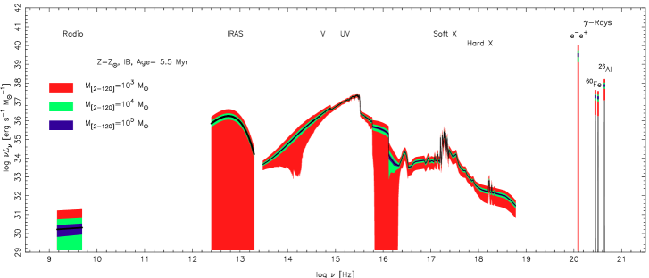
Figure 2.: Analytical 90% Confidence Level for the multiwavelength spectrum for a 5.5 Myr old burst.

Finally, there remains the problem of how to apply synthesis models to individual small systems. In this case, the situation is more complicated. Taking again the example of WR stars, whereas the presence of such stars enable us to quote an age range where the star formation began, their absence cannot be used to quote any plausible age range. However, if synthesis models have a physical reality, different observables must be related to each other. Hence, the real solution will lie in the joint distribution of the probability distributions of the different observables. Unfortunately, this kind of study has not yet been performed.

2.2. Starburts-AGN connection

In the preceding items I have shown that synthesis models must be applied with cautions to small systems. However, the definition of small depends on the statistics of the observable. In Cerviño, Mas-Hesse & Kunth (2002) we have computed the soft X-ray emission from starburst galaxies. This emission is produced from the reprocessing of the kinetic energy produced by the star forming regions and from the Supernova Remnants. In this case, the dispersion arises mainly from the occurrence of Supernova (SN) events, that is intrinsically a poor statistical observable: the SN rate is around 10^-9 SN yr^-1 M${}_{\odot}^{-1}$ (following a Salpeter IMF in the mass range 2 – 120 M_⊙, Cerviño & Mas-Hesse 1994), and the X-ray life time of an event is around 10⁴ yr, which implies $\cal M$ larger than 10⁵ in order to have a mean value of 1 SN active in X-rays. In that work the X-ray emission of individual SN events was averaged over the SN life time (see Aretxaga et al. in this proceedings for the statistics and evolution of SN fluxes), hence the quoted values are an average estimation with an additional dispersion that has not been considered. This additional dispersion may be relevant in the interpretation of the optical emission line spectrum in star forming galaxies (see also Rodríguez-Gaspar & Tenorio-Tagle 1998, Silich et al 2001, and Stasińska & Izotov 2002)

Besides the limitations, the approach is enough to test the relevance of circumnuclear star forming regions in the energy budget of Active Galactic nuclei (AGN). In Fig. 3, left panel, I show the soft-X ray/UV ratio predicted by the synthesis models and their comparison with the observational data of Star forming galaxies. In all the cases, some amount of kinetic energy must be reprocessed in X-ray in order to explain the observations. The comparison with Seyfert galaxies is shown in the right panel of the figure. Star forming regions are able to explain the X-ray emission of some Seyfert 2 galaxies, but their emission is not enough to explain the X-ray emission in Seyfert 1. In this approach, the putative black hole in some Seyfert 2 galaxies will only be relevant in the hard X-ray domain.

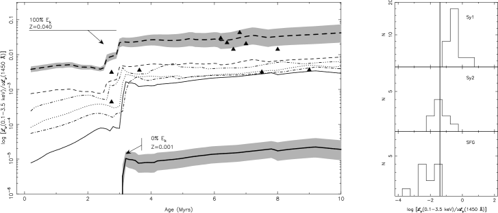
Figure 3.: Left: Ratio L_ν(0.1 – 3.5 keV) over $\nu$L_ν(1450 Å) computed for a 20% reprocessing values of mechanical energy into soft X rays and different metallicities. In grey, the 90% CL for a cluster where $10^{5}$ M_⊙ have been transformed into stars for two extreme metallicities and reprocessing values. Data points from star forming galaxies are marked as triangles. Right: Histograms for the ratio X-ray/UV for different types of emission line galaxies. The vertical solid line corresponds to the upper value predicted by our evolutionary synthesis models.

Acknowledgments.

I am gratefully for useful discussions with V. Luridiana, J.M. Mas-Hesse, E. Pérez, D. Valls-Gabaud, J.M. Vílchez, G. Stasińska and D. Kunth at different stages of this project. This project has been partially supported by the AYA 3939-C03-01 program. I also thank the LOC for financial support.

References

Bresolin, F., & Kennicutt, R. C. Jr. 2002, ApJ, 572, 838

Bruzual, G. 2002, in IAU Symp. 207, Extragalactic star clusters, eds. D. Geisler and E. Grebel (San Francisco: Astr. Soc. Pacific), in press (astro-ph/0110245)

Buzzoni, A. 1989, ApJS, 71, 871

Cerviño, M., Luridiana, V., & Castander, F. 2000, A&A, 360, L5

Cerviño, M., Valls-Gabaud, D., Luridiana, V., & Mas-Hesse, J.M. 2002, A&A, 381, 51

Cerviño, M., Mas-Hesse, J.M. & Kunth D. 2002, A&A, 392, 19

Cerviño, M., & Mollá 2002, A&A(accepted, astro-ph/0209147)

Cerviño, M., & Valls-Gabaud, D. 2002, MNRAS, (accepted, astro-ph/0209307)

Girardi, L., Bressan, A., Bertelli, G., & Chiosi, C. 2000, A&ASS, 141, 317

Rodríguez-Gaspar, J.A. & Tenorio-Tagle, G. 1998, A&A, 331, 347

Santos, J. F. C. Jr., & Frogel, J.A. 1997, ApJ,  479, 764

Stasińska G. & Izotov, Y.I. 2002, A&A (accepted, astro-ph/0209050)

Silich, S. A., Tenorio-Tagle, G., Terlevich, R., Terlevich, E. & Netzer, H. 2001, MNRAS, 324, 191

Tinsley, B. M., & Gunn, J. E. 1976, ApJ, 203, 52

Discussion

Dottori: How circumnuclear are the circumnuclear star forming regions you are talking about?

Cerviño: The data I have presented are based on IUE observations, so they are in a region of $10\times 20$ arc sec around the center.

Cid Fernandes: You have rightfully warned us that evolutionary synthesis predictions come with a statistical uncertainty. Have you compared your predictions for the variances with the observed dispersion in properties of star-forming regions?

Cerviño: Not personally. At this moment I am still working on the statistical implications. However, other authors (Bresolin & Kennicutt 2002) have applied the models results available on the Web server to high-metallicity star-forming regions and the theoretical dispersion looks to be consistent with the observed data.

García Vargas: It is true that taking into account all the probabilistic effects on cluster modeling is important to understand the dispersion, or degree of correlation when plotting observed data of GEHRs. However I think that this approach should be systematically applied to large GEHR where there is evidence of several small clusters ($<10^{5}$ M_⊙) from the region (as revealed from HST)

Cerviño: Yes, indeed the effect of sampling is more dramatic for low mass clusters (${\cal M}<10^{5}$ M_⊙), but it will be also present in more massive systems.