The evolution of stars and gas in starburst galaxies

Abstract

In systems undergoing starbursts the evolution of the young stellar population is expected to drive changes in the emission line properties. This evolution is usually studied theoretically, with a combination of evolutionary synthesis models for the spectral energy distribution of starbursts and photoionization calculations. In this paper we present a more empirical approach to this issue. We apply empirical population synthesis techniques to samples of Starburst and HII galaxies in order to measure their evolutionary state and correlate the results with their emission line properties. A couple of useful tools are introduced which greatly facilitate the interpretation of the synthesis: (1) an evolutionary diagram, whose axis are the strengths of the young, intermediate age and old components of the stellar population mix, and (2) the mean age of stars associated with the starburst, $\overline{t}_{SB}$. These tools are tested with grids of theoretical galaxy spectra and found to work very well even when only a small number of observed properties (absorption line equivalent widths and continuum colors) is used in the synthesis.

Starburst nuclei and HII galaxies are found to lie on a well defined sequence in the evolutionary diagram. Using the empirically defined mean starburst age in conjunction with emission line data we have verified that the equivalent widths of H$\beta$ and [OIII] decrease for increasing $\overline{t}_{SB}$. The same evolutionary trend was identified for line ratios indicative of the gas excitation, although no clear trend was identified for metal rich systems. All these results are in excellent agreement with long known, but little tested, theoretical expectations.

1 Introduction

Starburst systems in the local universe, from giant HII regions to Starburst nuclei, are important laboratories to study the evolution of massive stars and physical processes thought to be associated with the very early stages of galaxy formation. These motivations, coupled to the advances in modeling and observational capabilities, have led to a burst of activity in this field during the past decade.

By far the most common approach to infer the physical properties of starbursts is to compare their spectral energy distribution (SED) with models based on evolutionary synthesis (eg. Mas-Hesse & Kunth 1991; Olofsson 1995; Leitherer et al. 1999). This technique performs ab initio calculations of the spectral evolution of a stellar population on the basis of evolutionary tracks for stars covering a wide range of masses, stellar spectral libraries plus prescriptions for the initial mass function, star formation rate and chemical evolution. The comparison between observations and models may focus on particular spectral features, such as stellar wind lines in the UV (Robert, Leitherer & Heckman 1993), WR features (Cerviño & Mas-Hesse 1994; Schaerer & Vacca 1998), Balmer absorption lines (González Delgado, Leitherer & Heckman 1999), lines from red super giants (García-Vargas et al. 1997; Mayya 1997), or on a combination of lines and the multiwavelength continuum (Mas-Hesse & Kunth 1999; Lançon et al. 2001). A common difficulty faced in such studies is the contamination of the spectrum by an underlying old stellar population, which can be significant in the optical–near IR range. This contamination is sometimes removed by adopting a template spectrum for the old population (Lançon et al. 2001), or else its effects are evaluated from the excess flux between models and data (Mas-Hesse & Kunth 1999). Other uncertainties include those associated with differences between different sets of evolutionary tracks, incomplete or imperfect spectral libraries; stochastic effects and numerical issues (Cerviño et al. 2001); and possible effects of binary stars (Mas-Hesse & Cerviño 1999). We refer the reader to the review by Schaerer (2001) for a detailed discussion.

The massive, hot stars in young starbursts photoionize the surrounding gas, producing an emission line spectrum which can also be used to constrain the properties of the starburst, like its age, metallicity and star-formation rate. In fact, emission line diagnostics of starbursts play a central role in this field for the simple practical reason that emission lines are much easier to measure than stellar features. A great number of studies have been devoted to developing such diagnostics through a combination of theoretical SEDs from evolutionary synthesis and phototoionization calculations for the corresponding nebular conditions (García-Vargas, Bressan & Díaz 1995; Stasińska & Leitherer 1996; Charlot & Longhetti 2001; Moy, Rocca-Volmerange & Fioc 2001; Stasińska, Schaerer & Leitherer 2001; Schaerer 2000).

Among the many diagnostic tools developed, the equivalent width of H$\beta$ ($W_{H\beta}$) stands out as a powerful age indicator of starbursts. The prediction, known for more than 20 years (Dottori 1981), is that $W_{H\beta}$ decreases as a burst evolves. This behavior has been so extensively confirmed by more elaborate calculations that $W_{H\beta}$ is often used as a substitute for an age axis in studies which investigate the evolution of starbursts (e.g., Stasińska et al. 2001). Other general predictions of evolutionary synthesis + photoionization models are that the gas excitation and that the equivalent width of [OIII]$\lambda$5007 should decrease as a starburst evolves (Coppeti, Dottori & Pastoriza 1986; Stasińska & Leitherer 1996) although such diagnostics are more critically affected by metallicity effects.

These predictions, now routinely applied to infer physical properties of starbursts, are hard to be tested directly, since that requires evaluating the age of a starburst without resorting to emission line diagnostics. In this paper we take a step back in time and investigate the empirical validity of these long known predictions by means of a simple Empirical Population Synthesis (EPS) analysis of Starburst and HII galaxies. This analysis allows a quantitative assessment of the evolutionary state of a stellar population based only on observed stellar features. EPS techniques have their own limitations (eg, Cid Fernandes et al. 2001a), but these are of a different nature than the uncertainties involved in evolutionary synthesis, and thus serve as an independent test of predictions of evolutionary synthesis models.

Our main goals are to:

• Study the stellar population properties of a large and varied sample of star-forming galaxies by means of an EPS analysis.

• Develop and test EPS-based tools to assess the evolutionary state of star-forming galaxies in a quantitative and easy-to-interpret manner.

• Perform a model-independent investigation of the relation between gaseous properties and the evolutionary state of starbursts.

In section 2 we present the data sets used in this study. Section 3 deals with points (i) and (ii) above. The EPS method is presented and its results for star-forming galaxies are discussed by means of simple empirical tools designed to aid the interpretation of the synthesis. We also present a comparative study of EPS and evolutionary synthesis methods, which serves to test and calibrate our tools to measure evolution. In section 4 we address point (iii) by studying the evolution of emission line properties of Starburst and HII galaxies using an EPS-based measure of the burst age. Section 5 summarizes our main results.

2 Data

This investigation requires optical spectra where both gaseous (emission lines) and stellar properties (continuum and absorption lines) can be discerned. Two data sets meeting this requirement were used in this work.

The first set, which we denote “Sample I”, comes from the studies of Storchi-Bergmann, Kinney & Challis (1995) and McQuade, Kinney & Calzetti (1995), extracted from the atlas of Kinney et al. (1993). This sample covers both large, luminous galaxies with star-forming nuclei (“Starburst nuclei”) and smaller, weaker systems such as HII galaxies and blue compact dwarves. Active galaxies were discarded, with the exception of NGC 6221, which is dominated by Starburst activity except in X-rays (Levenson et al. 2001). We further limit our analysis to those objects with metallicity estimates by Storchi-Bergmann, Calzetti & Kinney (1994), which leaves a total of 41 galaxies, 18 of which are classified as Starburst nuclei. The spectra were collected through a large $10^{\prime\prime}\times 20^{\prime\prime}$ aperture, which corresponds to a circular aperture of 1.3 $h_{75}^{-1}$ kpc in radius at the median distance of the galaxies.

Emission line fluxes and equivalent widths ($W$) for this sample were re-measured from the publicly available original spectra and found to be in good agreement with those obtained by Storchi-Bergmann et al. (1995) and McQuade et al. (1995). All spectra were corrected for Galactic extinction using the reddening law of Cardelli, Clayton & Mathis (1989, with $R_{V}=3.1$) and the $E(B-V)$ values from Schlegel, Finkbeiner & Davis (1998) as listed in NED. Corrections for internal extinction were applied based on the H$\alpha$/H$\beta$ ratio, whose intrinsic value was taken to be 2.86, and allowing for underlying absorption components (see Section 4.1.1). For the stellar population analysis we have measured the $W$’s of the CaII K $\lambda$3933, CN $\lambda$4200 and G band $\lambda$4301 with respect to a pseudo continuum defined at selected pivot points, located at $\lambda=3660$, 3780, 4020 and 4510 Å, following the methodology outlined in Cid Fernandes, Storchi-Bergmann & Schmitt (1998). Our values agree very well with those of Storchi-Bergmann et al. (1995), but there were significant discrepancies between our measurements and those published by McQuade et al. (1995).

“Sample II” comes from the Spectrophotometric Atlas of HII galaxies of Terlevich et al. (1991), as analysed by Raimann et al. (2000a,b). Most of the individual spectra in this atlas do not have enough signal to measure stellar features, which prompted Raimann et al. to average them in order to increase the stellar signal. Out of 185 galaxies, they have defined 19 groups of similar characteristics. Each group is then treated as if it corresponded to an individual galaxy. Three of these groups are composed of Seyfert 2 galaxies. These were kept in our analysis only to illustrate their systematically different properties with respect to the remaining groups, 10 of which are composed of HII galaxies, 2 are Starburst nuclei and 4 are classified as intermediate HII/Staburst systems. The typical aperture covered by these spectra correspond to an equivalent radius of $0.8h_{75}^{-1}$ kpc.

Raimann et al. (2000a) have measured absorption line $W$’s and continuum fluxes for these groups following the same methodology as above. Emission line properties were analysed by Raimann et al. (2000b). Line fluxes were initially measured after subtraction of a stellar population model which included internal reddening. The resulting H$\alpha$/H$\beta$ ratio was used to further correct for residual extinction towards the line emitting regions. We have adopted both stellar and nebular properties as published by these authors without further corrections.

In summary, of all stellar and nebular properties compiled for these 2 samples, the following will be used in the analysis below: (1) the $W$’s of the CaII K, CN and G-band absorption features; (2) continuum fluxes at 3600, 4020 and 4510 Å; (3) emission line fluxes and $W$’s of strong optical lines: [OII]$\lambda$3727, H$\beta$, [OIII]$\lambda$5007, H$\alpha$ and [NII]$\lambda$6584; (4) nebular abundances, as listed in Storchi-Bergmann et al. (1994) and Raimann et al. (2000b); (5) the “activity class”, as reported in the afore mentioned papers. This last item is used to distinguish small systems like HII and blue compact galaxies from Starburst nuclei, which live on larger and more luminous galaxies, usually late type spirals. The latter kind of galaxies present a more complex mixture of stellar populations and are richer in heavy elements than HII galaxies, as will become clear in the analysis that follows.

3 Empirical Population Synthesis analysis

3.1 The method: input and output quantities

In order to provide a quantitative description of the stellar populations for galaxies in Samples I and II, we have used their absorption line $W$’s and continuum colors as input to the EPS algorithm developed by Cid Fernandes et al. (2001a). The code decomposes a spectrum onto a base of 12 simple stellar populations of different ages and metallicities ($Z$). This base was defined by Schmidt et al. (1991) out of a large sample of star clusters originally observed by Bica & Alloin (1986a,b). The main output of the code is the population vector ${\bf x}$, whose 12 components carry the fractional contributions of each base element to the observed flux at a given normalization wavelength $\lambda_{0}$. This vector corresponds to the mean solution found from a $10^{8}$ steps likelihood-guided Metropolis walk through the parameter space. Since colors are also modeled, extinction enters as an extra parameter, but this will not be directly used in our analysis. Some EPS studies (e.g., Bica 1988) impose that solutions follow well behaved paths on the age-$Z$ plane spanned by the base, in order to force consistency with simple scenarios for chemical evolution. Here we follow Schmidt et al. (1991) in not imposing such a priori constraints in order to allow for more general scenarios, such as systems undergoing mergers.

There are no major conceptual differences between this EPS method and that originally developed by Bica (1988) or its variants, which have been applied to many stellar population studies (e.g., Bica, Alloin & Schmidt 1990; De Mello et al. 1995; Kong & Cheng 1999; Schmitt, Storchi-Bergmann & Cid Fernandes 1999; Raimann et al. 2000a). However, in this work we will explore novel ways of expressing the results of the synthesis, which use the population vector to construct easy-to-interpret diagrams and indices.

The results presented below were all obtained feeding the EPS code with just 5 observables: The $W$’s of CaII K, CN and the G-band, plus the $F_{3660}/F_{4020}$ and $F_{4510}/F_{4020}$ continuum colors. The errors on these quantities were fixed at 0.5 Å for $W_{K}$ and $W_{G}$, 1 Å for $W_{CN}$, and 0.05 for the colors. As discussed by Cid Fernandes et al. (2001a), the combination of observational errors, little input information and quasi-linear dependences within the base hinders accurate estimates of all 12 components of ${\bf x}$, but reliable results are obtained grouping ${\bf x}$ components of same age. We have therefore employed age-grouping schemes in our analysis.

The base spans 5 logarithmicaly spaced age bins: $10^{6}$, $10^{7}$, $10^{8}$, $10^{9}$ and $10^{10}$ yr. Components with these ages are combined onto a reduced 5-D population vector, whose components are denoted by $x_{6}$, $x_{7}$, $x_{8}$, $x_{9}$ and $x_{10}$ respectively. We will also work with an even further reduced description of stellar populations, in which the $10^{9}$ and $10^{10}$ yr old components are re-grouped onto $x_{O}\equiv x_{9}+x_{10}$, and the young $10^{6}$ and $10^{7}$ yr components are binned onto $x_{Y}\equiv x_{6}+x_{7}$. Renaming the “intermediate age” $10^{8}$ yr component to $x_{I}\equiv x_{8}$, we obtain a compact, 3-D version of the population vector: $(x_{Y},x_{I},x_{O})$.

Normalization requires that $x_{Y}+x_{I}+x_{O}=1$, while the positivity constraint implies that all components are $\geq 0$. Therefore, an EPS solution is confined to a triangular cut of a plane in the $(x_{Y},x_{I},x_{O})$ space, which facilitates the visualization of results (see Cid Fernandes et al. 2001b for an application of this scheme to trace the evolution of circumnuclear starbursts in active galaxies). We note that the description of a galaxy spectrum in terms of ${\bf x}$-components is analogous to a Principal Component Analysis (e.g., Sodré & Stasińska 1999), with the difference that, by construction, each component has a known physical meaning.

We concentrate our analysis of the EPS results on evolutionary effects. Furthermore, we focus on the evolution of recent stellar generations ($\leq 10^{8}$ yr), associated with the star-forming activity in Starburst and HII galaxies. Metallicity effects are discussed using the nebular oxygen abundance, which essentially reflects the metallicity of the most recent stellar generation (Storchi-Bergmann et al. 1994).

3.2 EPS results and the evolutionary diagram

EPS Results for Samples I and II
Galaxy	$x_{6}$	$x_{7}$	$x_{8}=x_{I}$	$x_{9}$	$x_{10}$	$x_{Y}$	$x_{O}$	$\log\overline{t}_{SB}$ [yr]
ESO 296-11	22 $\pm$ 7	15 $\pm$ 8	29 $\pm$ 7	10 $\pm$ 5	23 $\pm$ 8	38 $\pm$ 6	33 $\pm$ 8	7.1 $\pm$ 0.9
ESO 572-34	28 $\pm$ 9	29 $\pm$ 11	16 $\pm$ 6	12 $\pm$ 5	15 $\pm$ 5	57 $\pm$ 5	27 $\pm$ 4	6.8 $\pm$ 0.5
1050+04	12 $\pm$ 6	12 $\pm$ 7	47 $\pm$ 8	11 $\pm$ 5	17 $\pm$ 6	24 $\pm$ 6	28 $\pm$ 6	7.5 $\pm$ 0.7
Haro 15	16 $\pm$ 7	21 $\pm$ 9	49 $\pm$ 7	6 $\pm$ 3	8 $\pm$ 5	37 $\pm$ 6	14 $\pm$ 5	7.4 $\pm$ 0.5
IC 1586	13 $\pm$ 7	22 $\pm$ 9	27 $\pm$ 7	21 $\pm$ 6	18 $\pm$ 7	35 $\pm$ 6	38 $\pm$ 6	7.2 $\pm$ 0.8
IC 214	11 $\pm$ 6	15 $\pm$ 7	37 $\pm$ 7	16 $\pm$ 6	22 $\pm$ 5	26 $\pm$ 5	38 $\pm$ 5	7.4 $\pm$ 0.6
Mrk 66	24 $\pm$ 6	10 $\pm$ 6	41 $\pm$ 7	7 $\pm$ 4	17 $\pm$ 4	34 $\pm$ 5	24 $\pm$ 5	7.2 $\pm$ 0.5
Mrk 309	16 $\pm$ 8	32 $\pm$ 10	25 $\pm$ 7	16 $\pm$ 5	12 $\pm$ 5	48 $\pm$ 6	28 $\pm$ 5	7.1 $\pm$ 0.5
Mrk 357	39 $\pm$ 10	31 $\pm$ 12	5 $\pm$ 3	13 $\pm$ 5	11 $\pm$ 4	70 $\pm$ 4	25 $\pm$ 3	6.5 $\pm$ 0.4
Mrk 499	16 $\pm$ 7	16 $\pm$ 8	50 $\pm$ 7	8 $\pm$ 4	10 $\pm$ 5	32 $\pm$ 6	18 $\pm$ 5	7.4 $\pm$ 0.5
Mrk 542	11 $\pm$ 6	16 $\pm$ 7	49 $\pm$ 8	10 $\pm$ 5	15 $\pm$ 6	27 $\pm$ 6	24 $\pm$ 6	7.5 $\pm$ 0.7
NGC 1140	20 $\pm$ 8	26 $\pm$ 10	35 $\pm$ 7	7 $\pm$ 4	12 $\pm$ 6	46 $\pm$ 6	19 $\pm$ 6	7.2 $\pm$ 0.6
NGC 1313	16 $\pm$ 7	19 $\pm$ 9	50 $\pm$ 7	5 $\pm$ 3	9 $\pm$ 5	35 $\pm$ 6	14 $\pm$ 5	7.4 $\pm$ 0.5
NGC 1510	8 $\pm$ 5	13 $\pm$ 6	57 $\pm$ 7	10 $\pm$ 5	11 $\pm$ 5	21 $\pm$ 5	22 $\pm$ 5	7.6 $\pm$ 0.6
NGC 1569	21 $\pm$ 9	44 $\pm$ 11	3 $\pm$ 2	25 $\pm$ 4	8 $\pm$ 4	65 $\pm$ 4	32 $\pm$ 3	6.7 $\pm$ 0.4
NGC 1614	16 $\pm$ 7	20 $\pm$ 9	39 $\pm$ 8	8 $\pm$ 4	17 $\pm$ 8	36 $\pm$ 6	25 $\pm$ 7	7.3 $\pm$ 0.7
NGC 1705	20 $\pm$ 9	34 $\pm$ 11	30 $\pm$ 7	7 $\pm$ 3	9 $\pm$ 5	54 $\pm$ 6	16 $\pm$ 5	7.1 $\pm$ 0.5
NGC 1800	10 $\pm$ 6	14 $\pm$ 7	55 $\pm$ 8	9 $\pm$ 4	13 $\pm$ 6	24 $\pm$ 6	22 $\pm$ 6	7.6 $\pm$ 0.6
NGC 3049	8 $\pm$ 6	31 $\pm$ 8	16 $\pm$ 6	26 $\pm$ 7	20 $\pm$ 8	39 $\pm$ 6	46 $\pm$ 6	7.1 $\pm$ 0.9
NGC 3125	21 $\pm$ 9	40 $\pm$ 11	17 $\pm$ 6	10 $\pm$ 4	11 $\pm$ 5	61 $\pm$ 6	22 $\pm$ 5	7.0 $\pm$ 0.5
NGC 3256	19 $\pm$ 8	29 $\pm$ 11	36 $\pm$ 7	6 $\pm$ 3	10 $\pm$ 5	48 $\pm$ 6	16 $\pm$ 5	7.2 $\pm$ 0.5
NGC 4194	10 $\pm$ 6	16 $\pm$ 7	39 $\pm$ 7	19 $\pm$ 6	16 $\pm$ 6	26 $\pm$ 5	35 $\pm$ 6	7.4 $\pm$ 0.7
NGC 4385	7 $\pm$ 5	26 $\pm$ 8	23 $\pm$ 7	24 $\pm$ 7	20 $\pm$ 8	33 $\pm$ 6	44 $\pm$ 7	7.3 $\pm$ 0.9
NGC 5236	10 $\pm$ 7	30 $\pm$ 9	35 $\pm$ 7	11 $\pm$ 5	13 $\pm$ 6	40 $\pm$ 6	25 $\pm$ 6	7.3 $\pm$ 0.6
NGC 5253	21 $\pm$ 10	46 $\pm$ 12	16 $\pm$ 6	8 $\pm$ 4	10 $\pm$ 5	67 $\pm$ 6	18 $\pm$ 5	6.9 $\pm$ 0.5
NGC 5860	12 $\pm$ 6	18 $\pm$ 8	22 $\pm$ 7	18 $\pm$ 8	30 $\pm$ 9	30 $\pm$ 6	49 $\pm$ 8	7.2 $\pm$ 1.1
NGC 5996	8 $\pm$ 5	20 $\pm$ 7	7 $\pm$ 4	28 $\pm$ 9	38 $\pm$ 9	28 $\pm$ 5	66 $\pm$ 6	7.0 $\pm$ 1.2
NGC 6052	10 $\pm$ 6	27 $\pm$ 9	32 $\pm$ 7	15 $\pm$ 6	16 $\pm$ 7	37 $\pm$ 6	31 $\pm$ 6	7.3 $\pm$ 0.7
NGC 6090	10 $\pm$ 6	20 $\pm$ 8	32 $\pm$ 7	29 $\pm$ 5	9 $\pm$ 4	30 $\pm$ 5	38 $\pm$ 4	7.4 $\pm$ 0.5
NGC 6217	9 $\pm$ 6	26 $\pm$ 8	20 $\pm$ 7	19 $\pm$ 7	26 $\pm$ 9	35 $\pm$ 6	45 $\pm$ 7	7.2 $\pm$ 1.0
NGC 6221	6 $\pm$ 5	19 $\pm$ 7	26 $\pm$ 8	24 $\pm$ 8	24 $\pm$ 9	25 $\pm$ 6	48 $\pm$ 7	7.4 $\pm$ 1.1
NGC 7250	20 $\pm$ 9	34 $\pm$ 11	25 $\pm$ 7	12 $\pm$ 4	9 $\pm$ 4	54 $\pm$ 6	21 $\pm$ 4	7.1 $\pm$ 0.4
NGC 7496	18 $\pm$ 7	17 $\pm$ 8	38 $\pm$ 8	10 $\pm$ 5	17 $\pm$ 7	35 $\pm$ 6	27 $\pm$ 7	7.3 $\pm$ 0.7
NGC 7552	7 $\pm$ 5	15 $\pm$ 7	48 $\pm$ 8	12 $\pm$ 5	18 $\pm$ 8	22 $\pm$ 6	30 $\pm$ 8	7.6 $\pm$ 0.8
NGC 7673	11 $\pm$ 6	19 $\pm$ 8	52 $\pm$ 8	6 $\pm$ 3	12 $\pm$ 7	30 $\pm$ 6	19 $\pm$ 7	7.5 $\pm$ 0.6
NGC 7714	17 $\pm$ 8	27 $\pm$ 10	33 $\pm$ 7	11 $\pm$ 5	12 $\pm$ 6	44 $\pm$ 6	23 $\pm$ 6	7.2 $\pm$ 0.6
NGC 7793	5 $\pm$ 4	12 $\pm$ 6	28 $\pm$ 8	23 $\pm$ 8	32 $\pm$ 10	17 $\pm$ 6	55 $\pm$ 8	7.5 $\pm$ 1.4
1941-543	23 $\pm$ 8	20 $\pm$ 9	40 $\pm$ 7	8 $\pm$ 4	9 $\pm$ 4	43 $\pm$ 5	17 $\pm$ 4	7.2 $\pm$ 0.4
Tol 1924-416	10 $\pm$ 7	45 $\pm$ 9	9 $\pm$ 5	19 $\pm$ 6	16 $\pm$ 6	56 $\pm$ 6	35 $\pm$ 5	7.0 $\pm$ 0.6
UGC 9560	31 $\pm$ 9	24 $\pm$ 10	13 $\pm$ 6	17 $\pm$ 6	15 $\pm$ 4	55 $\pm$ 5	32 $\pm$ 4	6.7 $\pm$ 0.5
UGCA 410	46 $\pm$ 6	9 $\pm$ 6	4 $\pm$ 3	6 $\pm$ 3	35 $\pm$ 3	55 $\pm$ 3	41 $\pm$ 2	6.3 $\pm$ 0.3
G_Cam1148-2020	91 $\pm$ 4	6 $\pm$ 4	1 $\pm$ 1	1 $\pm$ 1	2 $\pm$ 1	97 $\pm$ 1	3 $\pm$ 1	6.1 $\pm$ 0.1
G_UM461	84 $\pm$ 7	11 $\pm$ 7	1 $\pm$ 1	2 $\pm$ 1	3 $\pm$ 1	95 $\pm$ 2	4 $\pm$ 2	6.1 $\pm$ 0.1
G_Tol1924-416	59 $\pm$ 11	29 $\pm$ 12	5 $\pm$ 3	3 $\pm$ 2	4 $\pm$ 2	88 $\pm$ 4	7 $\pm$ 3	6.4 $\pm$ 0.3
G_NGC1487	56 $\pm$ 10	29 $\pm$ 12	8 $\pm$ 4	2 $\pm$ 2	4 $\pm$ 3	85 $\pm$ 5	7 $\pm$ 3	6.5 $\pm$ 0.3
G_Tol1004-296	47 $\pm$ 11	40 $\pm$ 12	4 $\pm$ 3	4 $\pm$ 2	5 $\pm$ 3	87 $\pm$ 4	9 $\pm$ 3	6.5 $\pm$ 0.3
G_UM488	42 $\pm$ 11	42 $\pm$ 12	6 $\pm$ 4	4 $\pm$ 2	6 $\pm$ 3	84 $\pm$ 5	9 $\pm$ 3	6.6 $\pm$ 0.3
G_Tol0440-381	45 $\pm$ 9	23 $\pm$ 11	22 $\pm$ 6	4 $\pm$ 2	7 $\pm$ 4	67 $\pm$ 6	11 $\pm$ 4	6.7 $\pm$ 0.4
G_UM504	35 $\pm$ 9	21 $\pm$ 10	25 $\pm$ 7	6 $\pm$ 3	13 $\pm$ 7	56 $\pm$ 6	19 $\pm$ 6	6.9 $\pm$ 0.6
G_UM71	22 $\pm$ 8	19 $\pm$ 9	38 $\pm$ 7	7 $\pm$ 4	14 $\pm$ 7	41 $\pm$ 6	21 $\pm$ 7	7.2 $\pm$ 0.7
G_NGC1510	16 $\pm$ 7	17 $\pm$ 9	51 $\pm$ 8	4 $\pm$ 3	12 $\pm$ 7	33 $\pm$ 6	16 $\pm$ 7	7.4 $\pm$ 0.6
G_Cam0949-2126	20 $\pm$ 8	21 $\pm$ 9	30 $\pm$ 7	13 $\pm$ 5	17 $\pm$ 6	41 $\pm$ 6	29 $\pm$ 6	7.1 $\pm$ 0.7
G_Mrk711	24 $\pm$ 10	38 $\pm$ 12	15 $\pm$ 6	8 $\pm$ 4	15 $\pm$ 7	62 $\pm$ 7	23 $\pm$ 6	6.9 $\pm$ 0.7
G_UM140	25 $\pm$ 8	16 $\pm$ 9	44 $\pm$ 7	4 $\pm$ 3	11 $\pm$ 6	41 $\pm$ 6	15 $\pm$ 6	7.2 $\pm$ 0.6
G_NGC3089	20 $\pm$ 7	12 $\pm$ 7	44 $\pm$ 8	5 $\pm$ 3	19 $\pm$ 9	32 $\pm$ 6	24 $\pm$ 8	7.3 $\pm$ 0.8
G_Mrk710	58 $\pm$ 11	30 $\pm$ 12	4 $\pm$ 3	3 $\pm$ 2	5 $\pm$ 3	87 $\pm$ 4	8 $\pm$ 3	6.4 $\pm$ 0.3
G_UM477	27 $\pm$ 8	20 $\pm$ 10	31 $\pm$ 8	6 $\pm$ 3	15 $\pm$ 7	47 $\pm$ 7	21 $\pm$ 7	7.1 $\pm$ 0.7
G_UM103	6 $\pm$ 5	10 $\pm$ 6	45 $\pm$ 8	15 $\pm$ 7	23 $\pm$ 8	17 $\pm$ 6	38 $\pm$ 8	7.6 $\pm$ 1.0
G_NGC4507	3 $\pm$ 2	6 $\pm$ 4	4 $\pm$ 3	26 $\pm$ 9	61 $\pm$ 9	9 $\pm$ 4	87 $\pm$ 4	7.1 $\pm$ 2.3
G_NGC3281	1 $\pm$ 1	4 $\pm$ 2	5 $\pm$ 3	39 $\pm$ 11	51 $\pm$ 11	5 $\pm$ 3	90 $\pm$ 4	7.3 $\pm$ 2.9

Table 1: Columns 2–6: Population vector in the $(x_{6},x_{7},x_{8},x_{9},x_{10})$ description. Columns 7, 4 and 8: $x_{Y}$, $x_{I}$ and $x_{O}$ respectively. All $x$ components are in percentages of the total flux at $\lambda_{0}=4020$ Å. Column 9: mean starburst age as defined in Section 3.4. Objects starting with a G_ are the spectral groups of Sample II. The three last entries in the table correspond to Seyfert 2 systems.

Figure 1: Results of the empirical population synthesis analysis for Samples I (a) and II (b), condensed on an evolutionary diagram. The horizontal axis $x_{Y}$ is the fraction of light at $\lambda_{0}=4020$ Å due to stars in the $10^{6}$ and $10^{7}$ yr age bins, while the fraction $x_{I}$ due to $10^{8}$ yr stars is plotted along the vertical axis. A third perpendicular axis carries the contribution $x_{O}$ of older populations ($\geq 10^{9}$ yr). Dotted lines indicate lines of constant $x_{O}$, as labeled. HII galaxies are plotted as triangles and Starburst nuclei as squares. Filled symbols correspond to galaxies with WR features. Crosses in panel (b) indicate Seyfert 2s. Note that the Starburst nucleus G_Mrk710 and the HII galaxy G_Tol1004_296, both of which show WR features, overlap at $(x_{Y},x_{I})=(0.87,0.04)$ in panel (b).

The results of the EPS analysis of galaxies in Samples I and II are listed in Table 1 both for the $(x_{6},x_{7},x_{8},x_{9},x_{10})$ and the Young, Intermediate and Old descriptions. The normalization wavelength is $\lambda_{0}=4020$ Å. A very convenient way to present the results of the synthesis is to project the $(x_{Y},x_{I},x_{O})$ vector onto the $x_{Y}$-$x_{I}$ plane. This is done in Figs. 1a and b for Samples I and II respectively. Dotted lines in these plots mark lines of constant $x_{O}$, computed from the $x_{Y}+x_{I}+x_{O}=1$ condition. Note that these are actually straight lines in the $x_{Y}$-$x_{I}$ plane, which appear curved because of the logarithmic axis.

Galaxies from both samples define a smooth sequence from large $x_{Y}$ to large $x_{I}$, with not much spread in $x_{O}$, particularly for Sample II. The larger spread seen in Fig. 1a is partly due to the fact that the data for Sample I was collected through apertures typically 2.6 times larger than for Sample II, and thus sample a more heterogeneous mix of stellar populations. This interpretation is supported by the fact that NGC 1510, which appears in both samples, looks somewhat younger in Sample II (see Table 1). Another source of scatter in Fig. 1a stems from the large number of Starburst nuclei in Sample I. These systems, represented by squares in both panels, live on galaxies with a significant old stellar component, whose effect is to drag points towards the bottom-left of the plot. For instance, the point at $(x_{Y},x_{I},x_{O})=(0.28,0.06,0.66)$ in Fig. 1a is NGC 5996, whose spectrum reveals a weak starburst immersed in an old population (McQuade et al. 1995; Kennicutt 1992). HII galaxies, on the other hand, are closer to “pure starbursts”. In fact, they were once thought to be truly young galaxies undergoing their first star-formation episode (Searle & Sargent 1972). Only recently it has become clear that they too contain old stars (Telles & Terlevich 1997; Schulte-Ladbeck & Crone 1998; Raimann et al. 2000a). This explains why Sample II, which is essentially an HII galaxy sample, exhibits a more well defined sequence in Fig. 1, with all non-AGN sources bracketed by the $x_{O}=0$ and 30% contours.

The three deviant crosses spoiling the Sample II sequence in Fig. 1b are the Seyfert 2 groups, with their predominantly old stellar populations (Raimann et al. 2000a). G_UM103 has a significant “post-starburst” component, reminiscent of more evolved starburst + Seyfert 2 composite systems, while the other two groups occupy a region characteristically populated by LINERs and non-composite Seyfert 2’s (Cid Fernandes et al. 2001b).

Since the location of a galaxy in Fig. 1 reflects the evolutionary state of its stellar population, we interpret the distribution of objects in this diagram as an evolutionary sequence, with the mean stellar age running counter-clockwise.

There are several reasons to interpret Fig. 1 as an evolutionary sequence. First, metal absorption lines become deeper and galaxy colors become progressively redder as one moves from large $x_{Y}$ to large $x_{I}$ along the sequence. In fact, the sequence defined by Sample II follows very closely the blue to red (young to old) spectral sequence in Figure 1 of Raimann et al. (2000a). Second, all Sample II galaxies in which WR features have been detected (those marked by filled symbols in Fig. 1b) are located in the large $x_{Y}$ region of the diagram, consistent with the young burst ages (a few Myr) implied by the mere presence of WR stars. Filled symbols in Fig. 1a mark galaxies from Sample I which are listed in the WR-galaxy catalog maintained by D. Schaerer (webast.ast.obs-mip.fr/people/scharer). Their more even distribution, as compared to Sample II, is due to the old population and aperture effects discussed above and nicely illustrated by Meurer (2000). Whereas the data analyzed here pertains to kpc-scales, spectra used to classify a starburst as a WR-galaxy are usually obtained through much narrower slits centered on the brightest cluster, thus favoring the detection of young systems. Processing such spectra through our EPS-machinery would surely move the filled points in Fig. 1a towards younger ages. (Conversely, one would expect that narrow slit observations of galaxies represented by empty symbols in the bottom right of Fig. 1a, such as Mrk 357 and UGCA 410, have a good chance of revealing WR features.) Finally, galaxies located in the large $x_{I}$ zone in the top-left (such as NGC 1800 in Sample I and group G_NGC3089 in Sample II) have spectra typical of a “post-starburst” population, with pronounced high order Balmer absorption lines typical of A stars (González Delgado et al. 1999). It is important to remark that neither the presence of WR features nor Balmer absorption lines were used in the EPS analysis, and yet the EPS results are compatible with the information apported by these observables.

3.3 EPS analysis of theoretical galaxy spectra

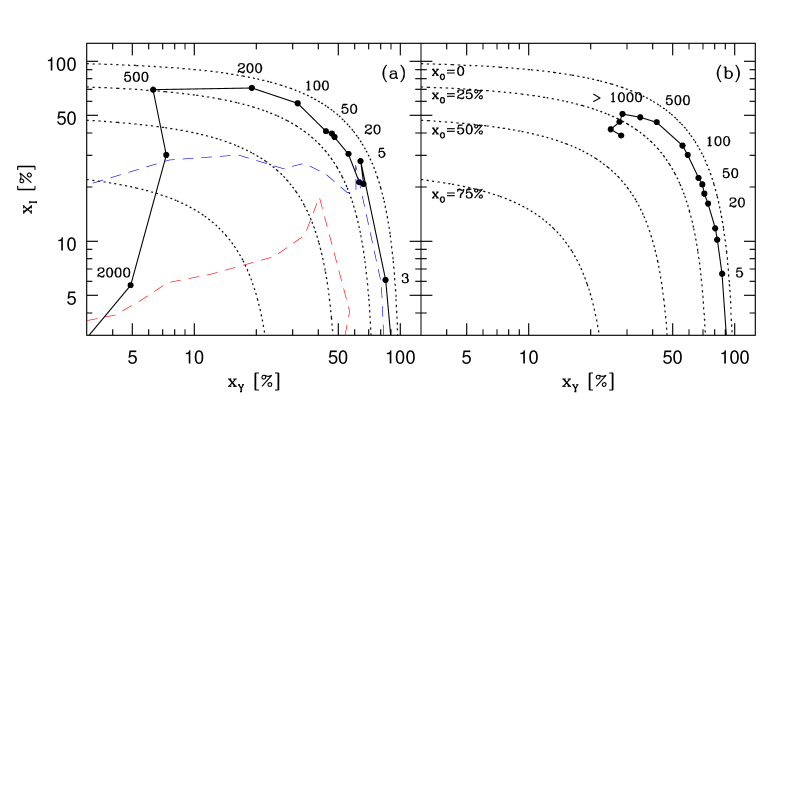
Figure 2: Evolution of GISSEL96 models on the $(x_{Y},x_{I},x_{O})$ EPS diagram, obtained processing the theoretical galaxies as the data. Dotted lines indicate lines of constant $x_{O}$. (a) The solid line shows results for an instantaneous burst. Numbers indicate the model age in Myr (note that evolution proceeds counterclockwise). Dashed lines correspond to instantaneous bursts on top of an old population which at $t=0$ accounts for $x_{Old}(0)=10\%$ (top) and 50% (bottom) of the flux at $\lambda_{0}=4020$ Å. (b) Models with continuous star formation.

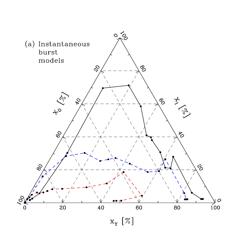
Figure 3: Evolution of GISSEL96 models in the $(x_{Y},x_{I},x_{O})$ EPS-space seen from a face on projection of the $x_{Y}+x_{I}+x_{O}=1$ plane. (a) Instantaneous burst models. The top curve corresponds to a pure burst, while the middle and bottom curves correspond to bursts atop a pre-existing old population with $x_{Old}(0)=10$ and 50% respectively. (b) Continuous star formation models.

A straight-forward theoretical reason to interpret Fig. 1 as an evolutionary sequence is that, schematicaly, a simple (i.e., coeval) stellar population moves on this diagram from $(x_{Y},x_{I},x_{O})=(1,0,0)$ at age $t=0$ to $(0,1,0)$ after some $10^{8}$ yr and then to $(0,0,1)$ for ages $\geq 10^{9}$ yr.

In order to follow this evolutionary path more closely we have carried out an EPS analysis of theoretical galaxy spectra from GISSEL96, the evolutionary synthesis code of Bruzual & Charlot (1993). The theoretical spectra were processed in exactly the same way as the real spectra of Samples I and II. Instantaneous burst and continuous star-formation models were computed for various ages between $t=0$ and 15 Gyr, a Salpeter IMF between 0.1 and 125 $M_{\odot}$ and $Z=Z_{\odot}$. GISSEL96 uses stellar tracks from the Padova group and offers a choice of spectral libraries. We have chosen the one which uses the atlas of Jacoby, Hunter & Christian (1984) for the optical range. The absorption features necessary for our EPS are clearly defined with this library. Spectral resolution was in fact the reason we have chosen GISSEL96 over the Starburst99 code of Leitherer et al. (1999), which is more taylored to study young stellar populations but currently works with an optical library too coarse for EPS analysis.

3.3.1 Burst models

The results for an instantaneous burst are shown as a solid line in the $(x_{Y},x_{I},x_{O})$ evolutionary diagram of Fig. 2a. Labels next to selected points indicate the model age in Myr. As expected, evolution proceeds from $x_{Y}$ to $x_{I}$ to $x_{O}$, such that a position on this diagram can be associated with an age. Fig. 3a provides an alternative representation of this diagram, in which all 3 components are explicitly plotted in a face-on projection of the plane containing the $(x_{Y},x_{I},x_{O})$ vector. The idea for this projection was borrowed from similar plots by Pelat (1997, 1998) and Moultaka & Pelat (2001).

In principle one would expect all evolution prior to ages of $\sim 10^{9}$ yr to progress along the $x_{O}=0$ contour, whereas in practice the GISSEL96 models oscillate between $x_{O}=10$ and 15% for $t<2\times 10^{8}$ yr. Similarly, the value of $x_{I}$ starts to increase before $t=10^{7}$ yr, when all stars should still belong to the $x_{Y}$ age bin. These deviations occur due to the limited number of observables used in the synthesis and because these contain observational errors which broaden the likelihood-function of ${\bf x}$ in a non-trivial way (Cid Fernandes et al. 2001a). As a result, some of the true $x_{Y}$ proportion always spills over onto $x_{I}$ and $x_{O}$, and so on. Overall, however, these figures show an excellent correspondance between empirical and evolutionary populations synthesis calculations.

In Fig. 4c we show the behavior of the 5 age components $x_{6}$–$x_{10}$ as a function of the age of the GISSEL96 models. The population vector evolves smoothly with age, except for the small kink a little short of $10^{7}$ yr due to the sudden appearance of red supergiants (Charlot & Bruzual 1991). As expected, $x_{6}$ peaks around $t=10^{6}$ yr, $x_{7}$ peaks around $t=10^{7}$ yr and so on, but note how $x_{7}$ is less well defined than any other component. The EPS decomposition tends to represent a $\sim 10^{7}$ yr burst as a combination of $x_{6}$ and $x_{8}$ instead of a strong $x_{7}$. Also, a non-negligible fraction of the $10^{6}$ yr component spills from $x_{6}$ onto $x_{7}$ for $t\mathrel{\hbox{\raise 2.15277pt\hbox{$<$}\hbox to0.0pt{\hss\lower 2.15277pt\hbox{$\sim$}}}}10^{6}$ yr. A similar effect occurs with $x_{9}$ and $x_{10}$ for $t\mathrel{\hbox{\raise 2.15277pt\hbox{$>$}\hbox to0.0pt{\hss\lower 2.15277pt\hbox{$\sim$}}}}10^{9}$ yr.

Such imprecisions in the mapping between evolutionary and empirical population synthesis are largely suppressed in the coarser, but more robust, $(x_{Y},x_{I},x_{O})$ description, as shown in Fig. 4b. The figure also shows the evolution of $x_{SB}=x_{6}+x_{7}+x_{8}$, which we hereafter treat as the “starburst component”, representing the past $\sim 10^{8}$ yr of the history of star formation in a galaxy. This is a more reasonable definition for our purposes than using only the youngest, ionizing population ($x_{6}$), since single burst models are not adequate to describe kpc scale regions such as those sampled by the observations of Samples I and II. Instead, the inner kpc of star-forming galaxies, particularly Starburst nuclei, contains a collection of many individual associations plus a field population with a spread in age. The detailed studies by Lançon et al. (2001) and Tremonti et al. (2001) illustrate this point (see also Calzetti 1997; Legrand et al. 2001). Such systems are frequently better represented by models with multiple bursts or continuous star formation over $\sim 10^{8}$ yr (Meurer 2000; Meurer 1995; Coziol, Barth & Demers 1995; Coziol, Doyon & Demers 2001).

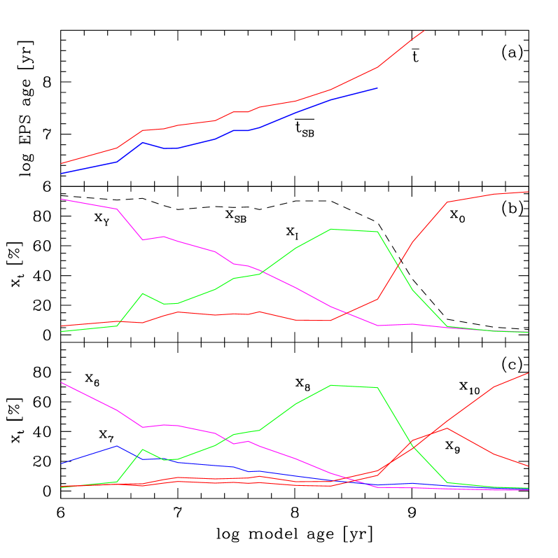
Figure 4: EPS parameters against model age for instantaneous burst models. (a) Mean ages, (b) population vector ${\bf x}$ in the reduced Young, intermediate and old description, and (c) in the 5 component description. The $\overline{t}_{SB}$ curve in (a) is stopped at a few times $10^{8}$ yr, after which it loses meaning for instantaneous bursts.

3.3.2 Burst plus an underlying old population

Real galaxies have a mixture of stellar populations of different ages, and galaxies in Samples I and II are no exception. The ongoing star-formation which makes them classifiable as starburst systems is observed atop an old ($\geq 10^{9}$ yr) stellar substrate formed in the earlier history of the galaxy. In our young, intermediate and old description, the effect of this underlying population is to dilute the values of $x_{Y}$ and $x_{I}$, which represent the recent history of star-formation. As a result, an instantaneous burst occurring on top of an old background does not follow the evolutionary sequence traced by the solid line in Fig. 2a.

Two quantities suffice to examine these diluting effects: the fraction $x_{Old}(0)$ of the total $L_{Burst}+L_{Old}$ luminosity at the start of the burst ($t=0$) which is due to old stars, and the function $l(t)=L_{Burst}(t)/L_{Burst}(0)$, which describes the luminosity evolution of the burst in units of its initial luminosity. Naturally, all these quantities refer to the same wavelength, $\lambda_{0}$. With these definitions, and considering that $L_{Old}$ does not evolve significantly on the time-scales of interest ($\leq 10^{8}$ yr), it is easy to show that

$$x_{Old}(t)=\frac{x_{Old}(0)}{x_{Burst}(0)l(t)+x_{Old}(0)}$$ (1)

where $x_{Burst}(0)=1-x_{Old}(0)$. We can now look at the evolution of ${\bf x}$ presented above for a pure burst as corresponding just to the $L_{Burst}(t)$ component, which at time $t$ accounts for only $x_{Burst}(t)=1-x_{Old}(t)$ of the total luminosity of the system. This allows us to, with the help of equation 1, re-normalize the evolution of $(x_{Y},x_{I},x_{O})$ to this new scale for any desired value of the contrast parameter $x_{Old}(0)$.

Results for $x_{Old}(0)=10$ and 50% are shown as dashed lines in Figs. 2a and 3a. As the burst fades, the evolutionary sequence bends over towards large $x_{O}$ quicker for larger $x_{Old}(0)$, i.e., for smaller initial ratios of burst to underlying old population power. Despite this effect, evolution still proceeds in an orderly counterclockwise fashion.

3.3.3 Continuous star-formation models

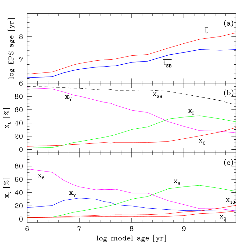
Figure 5: As Fig. 4 for models with continuous star formation.

Figs. 2b and 3b show the evolution of $(x_{Y},x_{I},x_{O})$ for GISSEL96 models with continuous star-formation. Since in this regime there are always young stars, at any given age $>0$ the system looks younger than an instantaneous burst model. At $t=10^{8}$ yr, for instance, $(x_{Y},x_{I},x_{O})\sim(0.6,0.3,0.1)$ for the continuous star-formation models and $(0.3,0.6,0.1)$ for an instantaneous burst. For $t>10^{9}$ yr, ${\bf x}$ converges to a region around $(0.3,0.4,0.3)$, instead of plunging towards large $x_{O}$ as for instantaneous bursts. Evolutionary sequences for models with time-decaying star-formation rates (say, exponentially or an “extended burst” step function), would define curves intermediary between those traced in Figs. 2a and b.

Since the luminosity increases without bounds for continuous star formation, any underlying old population is quickly outshone by the new stars. We therefore do not present dilution curves such as those computed for an instantaneous burst, since, except for the earliest ages, they are practically identical to the undiluted curves in Figs. 2b and 3b. The evolution of the population vector for continuous star-formation models is shown in Figs. 5b and c. As expected, the curves are smoother, and each component lives longer than for an instantaneous burst (Fig. 4).

3.4 Mean stellar age

The experiments above demonstrate that the evolutionary state of a starburst can be assessed by its location on the $(x_{Y},x_{I},x_{O})$ diagram. In order to translate this location into a number which quantifies the “evolutionary state” one could use, for instance, the angle $\theta=\tan^{-1}x_{I}/x_{Y}$, which increases as a burst evolves. Alternatively, we may use ${\bf x}$ to compute the mean age $\overline{t}$ of the stellar population. Since stellar populations evolve in a non-linear way, it makes more sense to define $\overline{t}$ from the mean $\log t$ among the populations represented by the base:

$$\log\overline{t}(\lambda_{0})\equiv\sum x_{i}(\lambda_{0})\log t_{i}$$ (2)

The dependence of ${\bf x}$ on the normalization wavelength is explicitly written in this equation to emphasize that this definition of $\overline{t}$ is $\lambda$-dependent. This happens because the $x_{i}$’s are flux fractions at $\lambda_{0}$, so $\overline{t}(\lambda_{0})$ is a flux-weighted mean age. A $\lambda$-dependent age makes observational sense for the simple reason that young stars are bluer than old stars, which makes $\overline{t}$ an increasing function of $\lambda$. Though the value of $\overline{t}$ depends on $\lambda_{0}$, the evolutionary sequence traced by this index independs on the choice of normalization, and so it can be used to rank populations on different evolutionary states.

For our 5-ages base ($t_{i}=10^{6}$, $10^{7}$, $10^{8}$, $10^{9}$ and $10^{10}$ yr), $\overline{t}(\lambda_{0})$ becomes (in yr)

$$\log\overline{t}(\lambda_{0})\equiv 6x_{6}+7x_{7}+8x_{8}+9x_{9}+10x_{10}$$ (3)

Since we are primarily interested in quantifying the evolutionary stage of populations associated with the most recent star-formation in starburst systems, it is interesting to consider a definition of $\overline{t}$ which removes the diluting effects of an underlying old stellar population. This can be done re-normalizing $x_{6}+x_{7}+x_{8}$ to 1, which yields the following definition for the mean starburst age (also in yr):

$$\log\overline{t}_{SB}(\lambda_{0})\equiv\frac{6x_{6}+7x_{7}+8x_{8}}{x_{6}+x_{7}+x_{8}}$$ (4)

Note that by construction $6\leq\log\overline{t}\leq 10$ and $6\leq\log\overline{t}_{SB}\leq 8$.

The solid lines in Fig. 4a compare our $\overline{t}$ and $\overline{t}_{SB}$ EPS-based age indices for $\lambda_{0}=4020$ Å with the corresponding age of the GISSEL96 models for an instantaneous burst. Despite some minor oscillations, these two indices bear a $\sim$ one-to-one relation with the theoretical age. Fig. 5a presents these same indices but for the continuous star-formation models. As expected, $\overline{t}$ and $\overline{t}_{SB}$ evolve more slowly than for an instantaneous burst, but they still increase steadily with the model age. Since $\overline{t}$ and $\overline{t}_{SB}$ are entirely obtained from a few easily measurable quantities, this result encourages their use as empirical clocks for stellar populations.

As it is clear from its very definition, due to the coarse age-resolution of the base, our mean age index $\overline{t}_{SB}$ is not meant to be used as a fine-graded chronometer of starbursts. Yet, the above experiments with theoretical spectra clearly show that $\overline{t}_{SB}$ provides a useful way to rank galaxies according to the age of the dominant population among the multiple generations of stars formed in the recent history of star-formation. This definition is particularly well suited to describe spectra which are integrated over large regions and hence average over many such generations, Although all galaxies discussed here contain populations younger than $10^{7}$ yr, which power their emission line spectrum, this ongoing star-formation may be less intense than in the recent past ($10^{7}$–$10^{8}$ yr), such that the young generations live among an older, non-ionizing starburst population. In this case, one expects to find significant $x_{7}$ and $x_{8}$ components, and thus $\overline{t}_{SB}>10^{7}$ yr. Conversely, if the current star-formation is more vigorous than in the past, mean ages of less than $10^{7}$ yr are expected. It is in this context of starbursts extended over a period of up to $\sim 10^{8}$ yr that we envisage $\overline{t}_{SB}$ and the $(x_{Y},x_{I},x_{O})$ diagram as useful tracers of evolution.

In principle, a base with a finer age resolution, including elements intermediate between $x_{6}$, $x_{7}$ and $x_{8}$, could yield a more detailed description of the evolution of starbursts. In practice, however, these elements would be well approximated by linear combinations of the existing base elements unless new observables were introduced in the synthesis process. For this reason, we opted to perform our EPS analysis with the base and observables described in §3.1, whose pros and cons have already been fully exploited in our previous investigations (Cid Fernandes et al. 2001a,b; Schmitt et al. 1999). Furthermore, as we shall soon see, this relatively coarse description is well suited to our present purposes.

4 The evolution of emission line properties

Emission lines in star-forming galaxies are umbilicaly linked to their young stellar population, whose massive, hot stars photoionize the surrounding gas. Also, in non-instantaneous starbursts the continuum carries a large contribution of stars borne before the current generation of ionizing stars, thus affecting emission line equivalent widths. In this section, we combine the tools to measure the evolution of starbursts developed in Section 3 with the emission line data compiled in Section 2 to investigate whether the emission line properties do indeed evolve along with the burst.

4.1 The equivalent width of H$\beta$

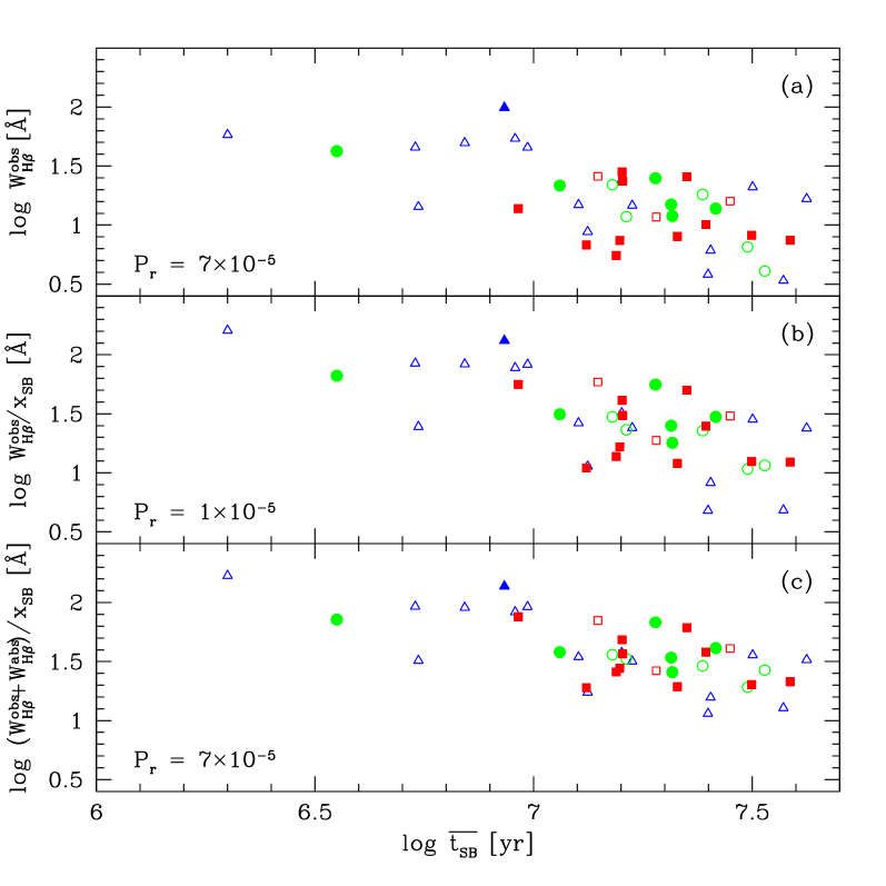
Figure 6: Equivalent width of H$\beta$ against the EPS-defined mean starburst age $\overline{t}_{SB}$ for Sample I. Panel (a) shows the observed equivalent widths ($W_{H\beta}^{obs}$). In (b) the contribution of old stars to the continuum under H$\beta$ is removed dividing $W_{H\beta}^{obs}$ by $x_{SB}(4861)$. In panel (c) $W_{H\beta}$ is further corrected for the presence of an absorption component. Triangles, circles and squares correspond to gas metallicity ranges of (O/H) $<0.4$, 0.4–0.6 and $>0.6$ (O/H)_⊙ respectively. Open and filled symbols are used to distinguish HII galaxies from Starburst nuclei. The $P_{r}$ values are the probabilities of no correlation in a Spearman test, small values indicating significant correlations.

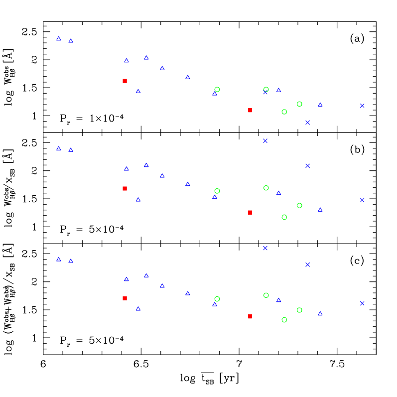
Figure 7: As Fig. 6 but for Sample II. Crosses indicate Seyfert 2’s, which were excluded from the correlation analysis.

As a burst ages, its most massive stars are the first to die, resulting in a steady decline of the ionizing photon flux and hence on the luminosity of recombination lines such as H$\beta$. The stellar continuum $C_{H\beta}$ underneath H$\beta$ also decreases, but more slowly than $L_{H\beta}(t)$, since it carries a significant contribution from longer-lived, non-ionizing, lower mass stars. As a result $W_{H\beta}=L_{H\beta}/C_{H\beta}$ decreases as the burst evolves, as first discussed by Dottori (1981) and confirmed by evolutionary synthesis calculations. $W_{H\beta}$ is therefore an age indicator, and it is frequently used as such in studies of star-forming systems (e.g, Stasińska et al. 2001). However, an empirical confirmation of the $W_{H\beta}(t)$ prediction requires an independent measure of the starburst age.

In Figs. 6a and 7a we carry out this test with galaxies from Samples I and II respectively, using our EPS-based index $\overline{t}_{SB}$ as a clock for the starburst. The anti-correlation between $W_{H\beta}$ and $\overline{t}_{SB}$ is evident for both samples, thus confirming that $W_{H\beta}$ decreases with time. The probability $P_{r}$ of no correlation in a Spearman’s rank test is just $7\times 10^{-5}$ for Sample I and $10^{-4}$ for Sample II, indicating a very high statistical significance. We emphasize that $W_{H\beta}$ and $\overline{t}_{SB}$ are determined from completely independent measurements, which only highlights the significance of this result.

The different symbols in Figs. 6, 7 and all subsequent plots represent three gas metallicity ranges, triangles, circles and squares corresponding to (O/H) $<0.4$, 0.4 to 0.6 and $>0.6$ (O/H)_⊙ respectively. Open and filled symbols are used to distinguish HII galaxies from Starburst nuclei. We postpone a discussion of the effects of $Z$ and activity class to Sections 4.3 and 4.4, which explore emission line properties more directly affected by these variables.

4.1.1 Corrections to $W_{H\beta}$

The values of $W_{H\beta}$ in Figs. 6a and 7a are the raw measurements ($W^{obs}_{H\beta}$). At least two corrections have to be considered, both of which increase $W_{H\beta}$.

(1) The continuum under H$\beta$ carries a contribution from an old stellar population which dilutes $W_{H\beta}$ with respect to the value it would have in a pure starburst. Our EPS analysis provides a natural way of correcting for this effect, which is a major source of concern in studies which use $W_{H\beta}$ as an age-indicator (Stasińska et al. 2001 and references therein). In order to isolate the contribution of the starburst to $C_{H\beta}$ it suffices to multiply it by $x_{SB}(4861)$, the starburst component defined in Section 3.3.1 but renormalized to $\lambda=4861$ Å. The corrected $W_{H\beta}$ is thus simply $W^{obs}_{H\beta}/x_{SB}(4861)$. Figs. 6b and 7b show the dilution-corrected evolution of $W_{H\beta}$.

The effects of this correction are largest for two of the Seyfert 2 groups in Sample II, which move significantly above the sequence in Fig. 7b because of their bulge dominated optical continuum (large $x_{O}$). The effect is not so large for G_UM103, which, as already discussed, resembles a starburst + Seyfert 2 composite. The fact that the observed values of $W_{H\beta}$ in Seyfert 2’s are in general smaller than those in starburst systems is purely due to this dilution effect. As explained by Cid Fernandes et al. (2001b), Seyfert 2’s ought to have intrinsically larger $W_{H\beta}$ than starbursts, as we obtain with our EPS-based dilution correction.

Among the star-forming galaxies in Samples I and II, this correction typically increases $W_{H\beta}$ by $\sim 50\%$ (in good agreement with the corrections inferred by Mas-Hesse & Kunth 1999 on similar objects), but it reachs more than a factor of 2 in some cases. The correction is somewhat smaller for Sample II, partly because it contains intrinsically younger systems and partly because of its smaller apertures, which reduces “contamination” by an extended old stellar population. The dilution correction improves the $W_{H\beta}$-$\overline{t}_{SB}$ correlation for Sample I and degrades the one for Sample II, while for the combined sample the statistical significance remains unchanged at $P_{r}=5\times 10^{-10}$.

(2) A second correction to be considered is that due to the presence of an absorption component hidden underneath the H$\beta$ emission. This component is present in our spectral base with strengths of up to $W^{abs}_{H\beta}=8$ Å, achieved for $10^{8}$ yr populations. We have used the population vector ${\bf x}$ obtained in the synthesis to compute the expected value of $W^{abs}_{H\beta}$, typically 3–5 Å. Adding $W^{abs}_{H\beta}$ to $W^{obs}_{H\beta}$ yields a corrected emission $W_{H\beta}$. The combined dilution and absorption corrected values of $W_{H\beta}$ are shown in Figs. 6c and 7c.

The absorption correction is only significant for galaxies with weak H$\beta$ emission, such as those bellow $W^{obs}_{H\beta}\sim 10$ Å at the bottom right of Fig. 6a. For these systems one has to look at the absorption-corrected values of $W_{H\beta}$ as uncertain by as much as a factor of 2. The correction is negligible for most galaxies in Sample II, which, due to its objective prism selection criterium, contains more strong lined objects than Sample I. Indeed, the mean $W^{obs}_{H\beta}$ is 55 Å for Sample II but just 22 Å for Sample I. This is also why, as a whole, Sample II contains a higher proportion of young starbursts.

The absorption correction degrades the $W_{H\beta}$-$\overline{t}_{SB}$ correlation for Sample I slightly. For the combined Sample I + II data the $P_{r}$ value increases from $5\times 10^{-10}$ to $3\times 10^{-8}$, which is still significant at the 5-$\sigma$ level. We thus see that these ‘1^st order corrections’ introduce very little scatter, and do not alter our conclusion that $W_{H\beta}$ does indeed evolve along with the stars that make up a starburst. One can also look at this result the other way around, and conclude that the fact that the $W_{H\beta}$ versus $\overline{t}_{SB}$ diagram behaves as expected proves the usefulness of our EPS-based evolutionary index $\overline{t}_{SB}$, with the advantage that it is immune to the dilution and absorption effects which plague $W_{H\beta}$ and other emission-line based age indicators.

We note in passing that these corrections alone are enough to bring the values of $W_{H\beta}$ within the range spanned by evolutionary synthesis calculations such as those by Leitherer et al. (1999), whereas, as it has long been known, the raw observed values fall bellow such predictions (Bressolin, Kennicutt & Garnett 1999 and references therein). Differential extinction, with line emitting regions being more reddened than the stellar continuum (Calzetti, Kinney & Storchi-Bergmann 1994) and leakage of ionizing photons out of the HII regions associated with the starburst are further examples of processes that act in the sense of reducing $W_{H\beta}$. We thus concur with Raimann et al. (2000b) and Stasińska et al. (2001) in that the apparent mismatch between theoretical and observed values of $W_{H\beta}$ bears no fundamental physical significance. In fact, the combined effects of differential extinction, leakage and the uncertainties in the dilution and absorption corrections are probably responsible for most of the vertical scatter in Figs. 6c and 7c.

4.1.2 Comparison with models

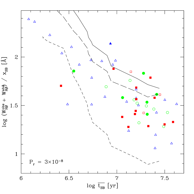
Figure 8: Observed and predicted evolution of $W_{H\beta}$. Data points are as in Figs. 6c and 7c. Lines correspond to theoretical $W_{H\beta}(t)$ curves with $t$ converted onto the EPS-based $\overline{t}_{SB}$ scale. Solid line: GISSEL96 models with a Salpeter IMF between 0.1 and 125 M_⊙. Dashed lines: Starburst99 models with a Salpeter IMF with M${}_{upp}=100$ M_⊙ (long dashes) and 30 M_⊙ (short dashes).

A quantitative comparison of the predicted evolution of $W_{H\beta}$ with that detected in Figs. 6 and 7 demands processing model spectra through the same EPS machinery used to analyse the data. This is necessary to translate model ages ($t$) onto our $\overline{t}_{SB}$ age scale. We have used the evolution of the rate of ionizing photons $N(H^{0})$ and the continuum under H$\beta$ predicted by GISSEL96 to compute $W_{H\beta}(t)$ for the same models synthesized in Section 3.3, for which the $t\rightarrow\overline{t}_{SB}$ conversion is shown in Figs. 4a and 5a.

The result for the continuous star formation models is shown as a solid line in Fig. 8, over-plotted onto the data points from Samples I and II (Figs. 6c and 7c). The dashed curves in this plot are the Starburst99 predictions (Leitherer et al. 1999) for solar metallicity, constant star formation models with a Salpeter IMF up to M${}_{upp}=100$ and 30 M_⊙. These latter curves are drawn with the $t\rightarrow\overline{t}_{SB}$ conversion obtained for GISSEL96, since, as already explained, it is not currently possible to do an EPS analysis with Starburst99 due to its poor spectral resolution optical libraries. Instantaneous burst models (not shown for clarity) follow roughly the same curves up to $\overline{t}_{SB}\sim 10^{6.8}$ yr and then plunge vertically, signaling the end of the ionizing phase of the cluster.

The rate at which $W_{H\beta}$ evolves is similar for models and data. Furthermore, practically all data points are bracketed by the models shown! Given the already discussed caveats affecting both axis of this figure, it would be premature to use this result to draw any conclusion about, say, the IMF in starbursts. The point to emphasize here is that, to our knowledge, this is the first time that predicted and observed values of $W_{H\beta}$ are plotted against an age axis, and it is gratifying to see a good agreement between data and models.

4.2 The equivalent width of [OIII]

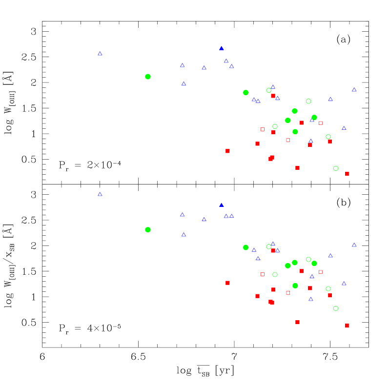
Figure 9: Equivalent width of [OIII]$\lambda$5007 against the mean starburst age $\overline{t}_{SB}$ for Sample I. Panel (a) shows the observed equivalent widths, whereas in (b) the dilution of $W_{[OIII]}$ by the underlying old stellar population is removed. Symbols as in Fig. 6.

The popularity of $W_{H\beta}$ as an age indicator stems mostly from its insensitivity to nebular conditions such as density, temperature and metallicity. Yet, the detailed photoionization models for evolving starbursts by Stasińska & Leitherer (1996) show that the equivalent width of [OIII] is also a powerful chronometer of starbursts for metallicities below solar, as is the case for most of the galaxies studied here. We therefore explore the behavior of $W_{[OIII]}$ against our empirical age index $\overline{t}_{SB}$.

The results for Sample I are shown in Fig. 9. An anti-correlation is clearly present. The relation gets even stronger after correcting $W_{[OIII]}$ for the dilution by an underlying population (Fig. 9b). Triangles and circles, which correspond to the two lower $Z$ bins, trace rather well defined sequences in Fig. 9b, but the more metal rich galaxies (plotted as squares) present a more scattered distribution. A plausible explanation for this larger spread is that, as discussed by Stasińska & Leitherer (1996), $W_{[OIII]}$ ceases to be a decreasing function of age as $Z$ approaches $Z_{\odot}$. Fig. 9b also shows that the higher $Z$ galaxies tend to have older starbursts, an effect which is further discussed below.

4.3 Gas excitation

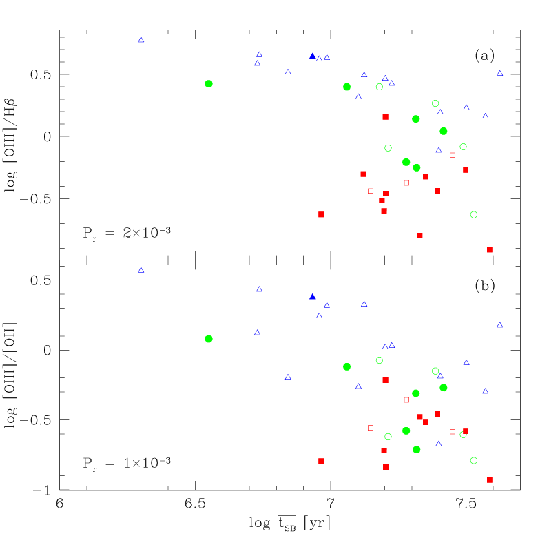
Figure 10: The evolution of gas excitation for Sample I galaxies, as measured by (a) [OIII]/H$\beta$ and (b) [OIII]/[OII]. Reddening and H$\beta$ absorption corrections were applied. Symbols as in Fig. 6.

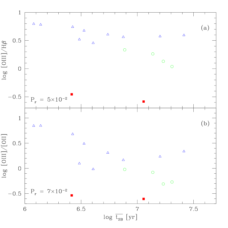
Figure 11: As Fig. 10 but for non-Seyfert galaxies in Sample II.

Another prediction of evolutionary synthesis plus photoionization calculations is that the gas excitation decreases with time, because the ratio of ionizing photons per gas particle (the “ionization parameter”) decreases and the ionizing spectrum softens as the hotter stars die (e.g., Copetti et al. 1986; Cid Fernandes et al. 1992; García-Vargas et al. 1995; Stasińska & Leitherer 1996). In Figs. 10 and 11 we explore the evolution of two line ratios in order to address this issue.

Unlike for emission line equivalent widths, particularly $W_{H\beta}$, metallicity plays a key role in defining ratios involving forbidden lines because of its influence on the gas temperature. The three $Z$ intervals represented by different symbols in these figures help to disentangle the effects of evolution and $Z$. Since HII galaxies are less chemically evolved than Starburst nuclei, differences in metallicity should also become apparent distinguishing objects by their activity class. This can be readily seen in Figs. 6–12. Most HII galaxies (open symbols) are in the low $Z$ bin (triangles), while most Starburst nuclei (filled symbols) are in the high $Z$ bin (squares). Sample I contains only one Starburst nucleus of the 16 sources with (O/H) $<0.4$ (O/H)_⊙ and only 3 HII galaxies among the 14 objects with (O/H) $>0.6$ (O/H)_⊙. For Sample II, the only two Starburst nuclei are also the most metal rich objects. Furthermore, the four (O/H) = 0.4–0.6 (O/H)_⊙ sources (open circles) located below the HII galaxy sequences in the $Z$-dependent Figs. 11a and b are precisely the four intermediate Starburst/HII galaxy groups defined by Raimann et al. (2000a). Metallicity and activity class are hence practically equivalent quantities.

Figs. 10 and 11 show the behavior of [OIII]/H$\beta$ and [OIII]/[OII] against $\overline{t}_{SB}$ for Samples I and II respectively. In this section we discuss only results for metal poor objects (triangles and circles), which are mostly HII galaxies. These systems present clear trends of decreasing excitation for increasing $\overline{t}_{SB}$, in qualitative agreement with theoretical predictions. Sources in Sample II join smoothly the sequences defined by sources in Sample I in all plots above, extending it to smaller $\overline{t}_{SB}$. As already explained, this happens mainly because of its objective prism selection, which favors the detection of young starbursts (e.g. Stasińska & Leitherer 1996). Since emission lines are powered solely by the most massive stars, they should be insensitive to the presence of older, non-ionizing populations, and hence we can expect the decrease in gas excitation to level off for $\overline{t}_{SB}>10^{7}$ yr. This is consistent with the distributions of low Z objects in Figs. 10 and 11. We have also investigated other line ratios, such as [OII]/H$\beta$ and [NII]/H$\alpha$, both of which increase systematically with increasing $\overline{t}_{SB}$.

These same trends, were identified and discussed by Stasińska et al. (2001), who used $W_{H\beta}$ as an age indicator. This agreement is hardly surprising, since we have empirically verified that $W_{H\beta}$ and our evolutionary index $\overline{t}_{SB}$ are related. In fact, as a corollary of this relation, we can automatically subscribe all trends found using $W_{H\beta}$ as measure of evolution! We therefore need not repeat here the extensive discussions on the evolution of emission line properties of starbursts by Stasińska et al. (2001) and previous studies. The usual caveats about reddening sensitive line ratios (such as [OIII]/[OII]) and the effects of an absorption component in H$\beta$, discussed in the references above, also apply here.

Of course, $\overline{t}_{SB}$ is a new age indicator, based entirely on measured stellar properties. Sure enough, it too has its limitations, but these are of a completely different nature than the uncertainties affecting emission line age diagnostics (e.g., the dilution correction for $W_{H\beta}$ or $W_{[OIII]}$). This reassuring agreement supports the interpretation of the trends in [OIII]/H$\beta$ and [OIII]/[OII] against $\overline{t}_{SB}$ for metal poor objects as a result of (theoretically expected) evolution of the gas excitation.

4.4 Metallicity effects

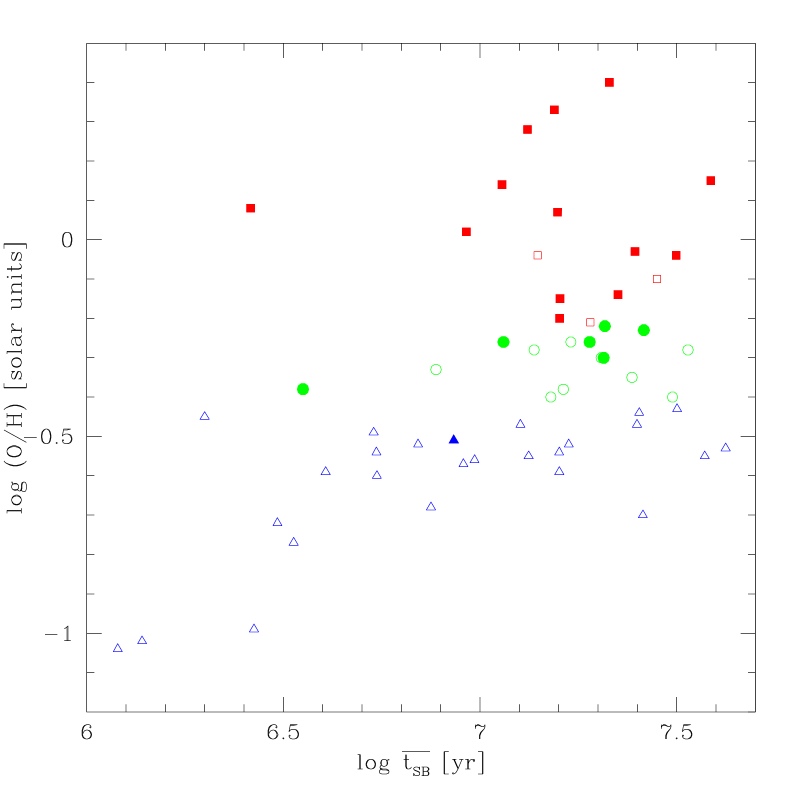
Figure 12: Gas metallicity against the evolutionary index $\overline{t}_{SB}$. Symbols as in Fig. 6. Starburst nuclei (filled symbols) are richer in metals than HII galaxies, and their mixed populations of $10^{6}$–$10^{8}$ yr stars make them look more evolved, producing the concentration towards to the top right.

Galaxies in our (O/H) $>0.6$ (O/H)_⊙ metal-rich bin, are heavily concentrated in the bottom-right regions of Figs. 6–12, corresponding to low emission line equivalent widths, low excitation and large age. Despite their horizontal offset towards large $\overline{t}_{SB}$, high $Z$ systems (plotted as squares) are well mixed with metal poor systems in the $W_{H\beta}$ diagrams (Figs. 6 and 7), in agreement with the idea that $W_{H\beta}$ is largely insensitive to $Z$. In the other diagrams, however, high $Z$ galaxies are clearly offset along the vertical axis, particularly in the gas-excitation plots (Figs. 10 and 11). Furthermore, while metal poor objects line up on broad but well defined sequences of decreasing $W_{[OIII]}$, [OIII]/H$\beta$ and [OIII]/[OII] for increasing $\overline{t}_{SB}$, no clear trends appear when considering high $Z$ objects by themselves. The scattered distribution of metal rich objects in these plots is in qualitative agreement with the models by Stasińska et al. (2001), which show that $Z$-dependent indices such as those used in Figs. 6–11 are not good chronometers for metal rich starbursts.

A more intriguing result is the systematic displacement of high $Z$ galaxies towards large $\overline{t}_{SB}$. A naive interpretation of this offset would be that these systems represent the late stages of evolution of metal poor starbursts. In this scenario, a triangle would become a circle and then a square in Figs. 6–11. Note, however, that this would require that (O/H) increases by factors of 3–10 in less than $10^{8}$ yr. Furthermore, this scenario would not be general, since there are several metal poor objects with large $\overline{t}_{SB}$. A more appropriate reading of Figs. 6–11 is that there is a wide spread in $Z$ for evolved starbursts, but there is practically no young metal rich system (the single exception being group G_Mrk710). This dichotomy is illustrated in Fig. 12, where $Z$ is plotted against $\overline{t}_{SB}$ for both samples.

We attribute this behavior to the fact that, as already explained, metal rich sources are predominantly Starburst nuclei, whereas HII galaxies dominate the lower $Z$ bins, as can be seen comparing the location of filled and open symbols in Fig. 12. In most HII galaxies the starburst population is dominated by the youngest generations, partly due to selection effects (see Section 4.1.1) and partly due to the fact that these are small galaxies, where a single burst can have a large impact. In fact, instantaneous burst models often provide an acceptable description of these systems, provided allowance is made for the presence of an old underlying population (Mas-Hesse & Kunth 1999). Starburst nuclei, on the other hand, present a more even distribution of stellar ages in the $10^{6}$–$10^{8}$ yr range (Lançon et al. 2001), more compatible with an extended star formation episode than with a coeval burst. This age mixture is detected by the synthesis, resulting in a skew of the $\overline{t}_{SB}$ index towards larger values.

We therefore conclude that the trend of $Z$ with $\overline{t}_{SB}$ simply reflects the fact that metal rich objects have a more complex recent history of star formation than metal poor objects.

5 Summary

We have investigated the evolution of emission line properties in Starburst nuclei and HII galaxies using age diagnostics based on their observed integrated stellar population properties. Our main results can be divided in two parts.

In the first part of this paper, we have presented the results of an empirical population synthesis (EPS) analysis of star-forming galaxies and explored ways to condense these results onto simple diagrams and indices designed to assess the evolutionary state of a stellar population. Two useful tools were developed:

• An evolutionary diagram: A compact description of stellar populations in terms of young ($\leq 10^{7}$ yr), intermediate age ($10^{8}$ yr) and old ($\geq 10^{9}$ yr) components allows the evolutionary state of a galaxy to be assessed by its location on a $(x_{Y},x_{I},x_{O})$ diagram, each axis carrying the contribution of stars within a given age range to the total flux.

• Mean ages: Flux–weighted mean ages of both the total stellar population ($\overline{t}$) and the starburst component ($\overline{t}_{SB}$) were defined .

Both tools were tested with theoretical galaxy spectra for instantaneous bursts and continuous star formation. These tests showed that the evolution of stellar populations is adequately mapped by these empirical tools, supporting their application to real galaxies. Perhaps the main conclusion here is that one can achieve a good first order description of the evolutionary state of a starburst using very little spectral information; our analysis used just 3 absorption lines plus 2 continuum colors in the 3600–4500 Å interval.

The EPS-analysis of two samples of starbursting galaxies showed them be distributed along the direction of evolution in the $(x_{Y},x_{I},x_{O})$ diagram. This result encouraged us to use our mean starburst age $\overline{t}_{SB}$ as an empirical clock to gauge the evolutionary state of starbursts.

In the second part of this study we have investigated correlations between the emission line properties of Starburst nuclei and HII galaxies and the $\overline{t}_{SB}$ index in order to test, in a completely empirical way, whether emission lines evolve along with the stars in starbursts. The results of this investigation can be summarized as follows.

• We have verified that the equivalent widths of H$\beta$ and [OIII] decrease for increasing $\overline{t}_{SB}$. This is in accordance with well known, but little tested, theoretical expectations.

• The use of $W_{H\beta}$ and $W_{[OIII]}$ as age indicators is hampered by the the diluting effects of an old underlying stellar population unrelated to the starburst. Besides providing a quantitative assessment of evolution, the EPS analysis provides a straight forward estimate of this effect.

• As a whole, Starburst nuclei are found to have a more even distribution of stellar ages in the $10^{6}$–$10^{8}$ yr range than HII galaxies, which are often dominated by the youngest generations.

• Three Seyfert 2 objects were also analysed, two of which have stellar population characteristics radically different from those in starburst galaxies, as seen, for instance, by their location on the evolutionary diagram. These two sources also have dilution-corrected $W_{H\beta}$ values well above those of starbursts. The third object has characteristics suggestive of a composite starburst + Seyfert 2 system.

• The gas excitation, as measured by emission line ratios, was found to decrease systematically for increasing $\overline{t}_{SB}$, also in agreement with theoretical predictions. This evolutionary sequence is only well defined for metal poor objects, which are mostly HII galaxies. Metal rich galaxies do not present clear evolutionary trends in the gas excitation indices, in qualitative agreement with photoionization models for evolving starbursts.

References

- [] Bica E., Alloin D., Schmidt A. A., 1990, A&A, 228, 23
- [] Bica E., 1988, A&A, 195, 76
- [] Bica E., Alloin D., 1986a, A&AS, 66, 171
- [] Bica E., Alloin D., 1986b, A&A, 162, 21
- [] Bresolin, F., Kennicutt, R. C., Garnett, D. R., 1999, ApJ, 510, 104
- [] Bruzual, A. G., Charlot, S. 1993, ApJ, 405, 538
- [] Calzetti, D., 1997, AJ, 113, 162
- [] Calzetti, D., Kinney, A. L., Storchi-Bergmann, T., 1994, ApJ, 429, 582
- [] Cardelli, J. A., Clayton, G. C., Mathis, J. S., 1989, ApJ, 345, 245
- [] Cerviño, M., Gómez-Flechoso, M. A., Castander, F. J., Schaerer, D., Mollá, M., Knödlseder, J., Luridiana, V., 2001, A&A, 376, 422
- [] Cerviño, M. & Mas-Hesse, J. M. 1994, A&A, 284, 749
- [] Charlot, S., Bruzual, A. G., 1991, ApJ, 367, 126
- [] Charlot, S., Longhetti, M. 2001, MNRAS, 323, 887
- [] Cid Fernandes, R., Dottori, H. A., Gruenwald, R. B., Viegas, S. M., 1992, MNRAS, 255, 165
- [] Cid Fernandes R., Storchi-Bergmann T., Schmitt H. R., 1998, MNRAS, 297, 579
- [] Cid Fernandes R., Heckman T., Schmitt H., Delgado R. M. G., Storchi-Bergmann T., 2001, ApJ, 558, 81
- [] Cid Fernandes R., Sodré L., Schmitt H. R., Leão J. R. S., 2001, MNRAS, 325, 60
- [] Copetti, M. V. F., Pastoriza, M. G., Dottori, H. A. 1986, A&A, 156, 111
- [] Coziol, R., Barth, C. S., Demers, S. 1995, MNRAS, 276, 1245
- [] Coziol, R., Doyon, R., Demers, S. 2001, MNRAS, 325, 1081
- [] de Mello D. F., Keel W. C., Sulentic J. W., Rampazzo R., Bica E., White R. E., 1995, A&A, 297, 331
- [] Dottori H. A., Bica E., 1981, A&A, 102, 245
- [] Garcia-Vargas, M. L., Bressan, A., Diaz, A. I., 1995, A&AS, 112, 35.
- [] García-Vargas M. L., Bressan A., Diaz A. I., 1995, A&AS, 112, 13
- [] González Delgado, R. M., Leitherer, C., Heckman, T. M., 1999, ApJS, 125, 489
- [] Kinney, A. L., Calzetti, D., Bohlin, R. C., McQuade, K., Storchi-Bergmann, T., Schmitt, H. R. 1996, ApJ, 467, 38
- [] Kong X., Cheng F. Z., 1999, A&A, 351, 477
- [] Lançon, A., Goldader, J. D., Leitherer, C., Delgado, R. M. G., 2001, ApJ, 552, 150
- [] Legrand, F., Tenorio-Tagle, G., Silich, S., Kunth, D., Cerviño, M., 2001, ApJ, 560, 630
- [] Leitherer C., Schaerer D., Goldader J. D., Delgado R. M. G., Robert C., Kune D. F., de Mello D. F., Devost D., Heckman T. M., 1999, ApJS, 123, 3
- [] Levenson N. A., Cid Fernandes R, Weaver K. A., Heckman T. M., Storchi-Bergmann T., 2001, ApJ, 557, 54
- [] Mas-Hesse, J. M., Kunth, D., 1991, A&AS, 88, 399
- [] Mas-Hesse, J. M., Kunth, D., 1999, A&A, 349, 765
- [] Mas-Hesse, J. M., Cerviño, M. 1999, IAU Symp., 193, 550
- [] Meurer, G. R., Heckman, T. M., Leitherer, C., Kinney, A., Robert, C., & Garnett, D. R. 1995, AJ, 110, 2665
- [] Meurer, G. 2000, in “Massive Stellar Clusters”, Eds. A. Lançon and C. Boily, ASP Conf. Series, p. 81
- [] McQuade K., Calzetti D., Kinney A. L., 1995, ApJS, 97, 331
- [] Moultaka, J., Pelat, D., 2000, MNRAS, 314, 409
- [] Moy, E., Rocca-Volmerange, B., Fioc, M. 2001, A&A, 365, 347
- [] Olofsson, K., 1995, A&AS, 111, 57
- [] Pelat D., 1997, MNRAS, 284, 365
- [] Pelat D., 1998, MNRAS, 299, 877
- [] Raimann, D, Storchi-Bergmann, T., Bica, E., Melnick, J., Schmitt, H., 2000, MNRAS, 316, 559
- [] Raimann D., Bica E., Storchi-Bergmann T., Melnick J., Schmitt H., 2000,MNRAS, 314, 295
- [] Robert, C, Leitherer, C., Heckman, T. M., 1993, ApJ, 418, 749
- [] Schaerer, D., Vacca, W. D., 1998, ApJ, 497, 618
- [] Schaerer, D. 2001, Starburst Galaxies: Near and Far, 197
- [] Schaerer, D., Guseva, N. G., Izotov, Y. I., Thuan, T. X. 2000, A&A, 362, 53
- [] Schlegel D. J., Finkbeiner D. P., Davis M., 1998, ApJ, 500, 525
- [] Schmidt A. A., Copetti M. V. F., Alloin D., Jablonka P., 1991, MNRAS, 249, 766
- [] Schmitt H. R., Storchi-Bergmann T., Cid Fernandes R. C., 1999, MNRAS, 303, 173
- [] Stasińska G., Leitherer C., 1996, ApJS, 107, 661
- [] Stasińska, G., Schaerer, D., Leitherer, C. 2001, A&A, 370, 1
- [] Storchi-Bergmann T., Kinney A. L., Challis P., 1995, ApJS, 98, 103S,
- [] Storchi-Bergmann T., Calzetti D., Kinney A. L., 1994, ApJ, 429, 572
- [] Terlevich R., Melnick J., Masegosa J., Moles M., Copetti M. V. F., 1991, A&AS, 91, 285
- [] Tremonti, C. A., Calzetti, D., Leitherer, C., Heckman, T. M., 2001, ApJ, 555, 322