Iron abundances and heating of the ICM in hydrodynamical simulations of galaxy clusters

Abstract

Results from a large set of hydrodynamical smoothed-particle-hydrodynamic (SPH) simulations of galaxy clusters in a flat $\Lambda$CDM cosmology are used to investigate the metal enrichment and heating of the intracluster medium (ICM). The physical modeling of the gas includes radiative cooling, star formation, energy feedback and metal enrichment that follow from the explosions of supernovae of type II and Ia. The metallicity dependence of the cooling function is also taken into account. The gas is metal enriched from star particles according to the SPH prescriptions. The simulations have been performed to study the dependence of final metal abundances and heating of the ICM on the numerical resolution and the model parameters.

For a fiducial set of model prescriptions the results indicate radial iron profiles in broad agreement with observations; global iron abundances are also consistent with data. It is found that the iron distribution in the intracluster medium is critically dependent on the shape of the metal deposition profile. At large radii the radial iron abundance profiles in the simulations are steeper than those in the data, suggesting a dynamical evolution of simulated clusters different from those observed. For low temperature clusters simulations yield iron abundances below the allowed observational range, unless it is introduced a minimum diffusion length of metals in the ICM. The simulated emission-weighted radial temperature profiles are in good agreement with data for cooling flow clusters, but at very small distances from the cluster centres ($\sim 2\%$ of the virial radii) the temperatures are a factor $\sim$ two higher than the measured spectral values.

The luminosity-temperature relation is in excellent agreement with the data, cool clusters ($T_{X}\sim 1keV$) have a core excess entropy of $\sim 200keVcm^{2}$ and their X-ray properties are unaffected by the amount of feedback energy that has heated the ICM. The findings support the model proposed recently by Bryan, where the cluster X-ray properties are determined by radiative cooling. The fraction of hot gas $f_{g}$ at the virial radius increases with $T_{X}$ and the distribution obtained from the simulated cluster sample is consistent with the observational ranges.

1 INTRODUCTION

Galaxy clusters are the largest virialized structures known in the universe and are considered useful probes to constrain current cosmological theories of structure formation. X-ray observations of galaxy clusters show that most of the baryonic cluster mass is in the form of a hot ionized intracluster medium at temperatures $\simeq 10^{7}-10^{8}~{}\kern 2.0pt{}^{\circ}{\kern-2.0ptK}$, with the bulk of the emission in the X-ray band from bremsstrahlung processes [Sarazin 1986]. The dependence of the X-ray emission on the square of the gas density allows us to construct cluster samples without the biases which may arise in the optical band. The final physical state of the ICM is primarily determined by the gravitational processes, which have driven the dynamical evolution of the gas and dark matter mass components during the cluster collapse. Under the assumption of hydrostatic equilibrium the ICM gas distribution can be modeled to connect the gas temperature $T_{X}$ to the cluster virial mass or to the bolometric X-ray luminosity $L_{X}$. The X-ray temperature and luminosity functions are then predicted for a given cosmological model according to the standard theoretical Press-Schecter (1974) mass function. The observed evolutionary history of these functions [Edge et al. 1990, Henry & Arnoud 1991, Henry 1997] can then be used to put severe constraints on the allowed cosmological models [Henry & Arnoud 1991, White, Efstathiou & Frenk 1993, Eke, Cole & Frenk 1996, Bahcall & Fan 1998, Kitayama, Sasaki & Suto 1998].

If the ICM has been shock heated solely by gravitational processes, the cluster scaling relations are predicted to obey a self-similar behavior. For instance, the $L_{X}-T_{X}$ relation should scale as $L_{X}\propto T_{X}^{2}$ [Kaiser 1986]. For clusters with $T_{X}\lower 2.15277pt\hbox{$\;\buildrel>\over{\sim}\;$}2keV$ there is a wide observational evidence [David et al. 1993, Allen & Fabian 1998, Markevitch 1998] that the observed bolometric X-ray luminosity scales with temperature with a slope steeper than expected ($L_{X}\propto T_{X}^{3}$). This implies that low temperature clusters have central densities lower than those predicted by the self-similar scaling relations [Bower 1997, Ponman, Cannon & Navarro 1999, Lloyd–Davies, Ponman & Cannon 2000]. This break of self-similarity is usually taken as a strong evidence that non-gravitational heating of the ICM has played an important role in the ICM evolution [Evrard & Henry 1991, Kaiser 1991, White 1991], at least for cool clusters.

The most considered source of energy which has been considered as a heating mechanism for the ICM is supernovae (SNe) driven-winds, which inject energy into the ICM through SNe explosions of type Ia and II [White 1991, Loewenstein & Mushotzky 1996]. The energy input required to heat the gas at the entropy level necessary to reproduce the observed departure from self-similarity is estimated to lie in the range $\simeq 0.5-3keV$ per particle [Balogh, Babul & Patton 1999, Wu, Fabian & Nulsen 2000, Tozzi & Norman 2001]. Several authors have argued that it is unlikely that SNe can provide the required energy to heat the gas and have suggested active galactic nuclei [Valageas & Silk 1999, Wu, Fabian & Nulsen 2000], as the extra energy source for ICM heating. Bryan (2000) has proposed the alternative view that radiative cooling and the subsequent galaxy formation [Pearce et al. 2000], can explain the observed $L_{X}-T_{X}$ relation because of the removal of low-entropy gas at the cluster cores.

The estimates of the energy injected from SNe into the ICM are based on the measured abundances of metals in the ICM. The elements that have enriched the ICM have been synthesized in the SNe explosions of the stellar population of the cluster. Two enrichment mechanisms have been proposed: supernova-driven galactic winds from early-type galaxies [Mushotzky & Lowenstein 1997], or ram pressure stripping of the enriched gas from galaxies [Gunn & Gott 1972]. Another possibility is that of a significant contribution to the metal enrichment and heating of the ICM, associated with an early-epoch generation of massive Population III stars [Loewenstein 2001].

A large set of observations confirms that the ICM of galaxy clusters is rich in metals [Arnaud et al. 1992, Mushotzky & Lowenstein 1997, Fukazawa et al. 1998, Dupke & White 2000a, Finoguenov, David & Ponman 2000, Fukazawa et al. 2000, Matsumoto et al. 2000]. Analyses of X-ray spectra show that the abundance of heavy elements in the ICM is nearly $\simeq 1/3$ solar. These measurements provide a strong support for the SN scenario as a heating source for the ICM.

Abundance gradients have also been measured [Ezawa et al. 1997, Dupke & White 2000b, White 2000, Finoguenov, David & Ponman 2000, De Grandi & Molendi 2001, Irwin & Bregman 2001]. For instance Ezawa et al. (1997) found a decline in the iron abundance of AWM7 from $\simeq 0.5$ solar in the centre to $\simeq 0.2$ solar at a distance of $\simeq 500Kpc$. Measurements of the relative abundance of the heavy elements can be used to constrain the enrichment mechanism of the ICM and the energy input from SNe. Analysis of the spatial distribution of metallicity gradients is also important to discriminate among the proposed enrichment scenarios [Dupke & White 2000b]. From the observed metallicities one can estimate the SN energy released given a shape for the initial-mass-function (IMF) and a nucleosynthesis yield model for the SN explosions. Finoguenov, Arnaud & David (2001) have obtained the Si and Fe abundances using the X-ray data of a selected sample of X-ray clusters. From the measured abundances, they find a significant contribution to the energy per particle associated with SNe explosions at temperatures $\simeq 3keV$.

These kinds of estimates of the SN energy input suffer from the theoretical uncertainties in the yield models and in the form of the IMF [Gibson, Loewenstein & Mushotzky 1997]. Moreover, these estimates can vary widely with the assumed spatial distribution of the ICM metals and the transfer efficiency of the kinetic energy released in a SN explosion to the ambient gas [Kravtsov & Yepes 2000]. Hydrodynamical simulations of cluster evolution have the advantage over analytical methods that they take into account the dynamical evolution of the gas. From the results of numerical simulations of galaxy formation, Kravtsov & Yepes (2000) conclude that it is unlikely that SNe can provide the required energy input, even assuming the existence of radial metallicity gradients in the ICM.

In order to implement self-consistently the metal enrichment of the ICM in hydrodynamical simulations of galaxy clusters, one first must consider the effects of non-gravitational processes on the cluster gas distribution. The effects of radiative cooling in simulated clusters have been investigated by a number of authors [Anninos & Norman 1996, Lewis et al. 2000, Pearce et al. 2000, Yoshikawa, Jing & Suto 2000, Valdarnini 2002]. One of the main conclusions of these simulations is that the modeling of radiative processes for the gas cannot be decoupled from a prescription for turning cold, dense gas into stars. This is done in order to avoid unphysically high densities (cooling catastrophe). The luminosities $L_{X}$ of the simulated clusters are found to be physically plausible, provided that a suitable prescription for the treatment of the cold gas has been taken into account.

In a previous paper [Valdarnini 2002] results from a set of hydrodynamical SPH simulations of galaxy clusters have been used to investigate how final X-ray properties of the simulated clusters depend upon the simulation numerical resolution and the chosen star formation (SF) prescription. For a chosen SF model, final X-ray luminosities have been found to be numerically stable and consistent with data, with uncertainties of a factor $\simeq 2$. In these simulations the metal enrichment of the ICM has been included with a minimal number of prescriptions and it was shown that for the simulated clusters, the final iron abundances of the ICM are in broad agreement with measured values.

Chemical evolution in hydrodynamical SPH simulations has already been considered in a variety of contexts [Steinmetz & Müller 1994, Raiteri, Villata & Navarro 1996, Carraro, Lia & Chiosi 1998, Buonomo et al. 2000, Mosconi et al. 2001, Churches, Nelson & Edmunds 2001, Lia, Portinari & Carraro 2002, Aguirre et al. 2001]. Metzler & Evrard (1994) have investigated the metal enrichment of the ICM in P3MSPH simulations of galaxy clusters in a standard cold dark matter (CDM) scenario. The authors have not included radiative cooling in the simulations and have adopted a phenomenological prescription to model the chemical enrichment.

In a more recent paper, Kravtsov & Yepes (2000) have estimated SN heating of the ICM using fixed-grid Eulerian hydrodynamical simulations. However, the numerical resolution of the simulations was not adequate to study the evolution of simulated clusters. The number of SNe occurring in a given cluster was estimated statistically from many small-box galaxy formation simulations. The implementation of a self-consistent metal enrichment model for the ICM in hydrodynamical simulations is therefore important for investigations of the ICM metal evolution. This is particularly relevant in connection with the observed metallicity gradients and for assessing the reliability of the calculated amount of ICM heating from SNe, inferred from measured metallicity abundances.

The main aim of this paper is to analyze, in hydrodynamical SPH simulations of galaxy clusters, the dependence of the final iron abundance on a number of model parameters that control the ICM metal enrichment. This is done in order to obtain for the simulated clusters a final ICM distribution which can consistently fit a set of observational constraints, such as the observed iron abundances and at the same time the luminosity-temperature relation. Implications for the ICM heating from SNe are also discussed. This paper constitutes a generalization of a previous work (Valdarnini 2002, hereafter V02), where the investigation was mainly concerned with the numerical stability of different SF models. Section 2 presents the hydrodynamical simulations of galaxy clusters that have been performed. Section 3 describes the star formation algorithm and the modeling of ICM metal enrichment implemented in the simulations. Results are presented in Section 4 and the conclusions in Section 5.

2 SIMULATIONS

Here I give a short description of the simulations. Further details can be found in V02.

The cosmological model considered is a flat CDM model, with a vacuum energy density $\Omega_{\Lambda}=0.7$, matter density parameter $\Omega_{m}=0.3$ and Hubble constant $h=0.7$ in units of $100Kmsec^{-1}Mpc^{-1}$. The primeval spectral index of the power spectrum $n$ is set to $1$ and $\Omega_{b}=0.015h^{-2}$ is the value of the baryonic density. The power spectrum of the density fluctuations has been normalized in order to match at the present epoch the measured cluster number density [Eke, Cole & Frenk 1996, Girardi et al. 1998]. Initial conditions for the cluster simulations are constructed as follows. A collisionless cosmological N-body simulation is first run in a $L=200h^{-1}Mpc$ comoving box using a P3M code with $84^{3}$ particles, starting from an initial redshift $z_{in}$. At $z=0$ cluster of galaxies are located using a friend-of-friend algorithm, so to detect densities $\simeq 200\Omega_{m}^{-0.6}$ times the background density within a radius $r_{200}$. The corresponding mass $M_{200}$ contained within this radius is defined as $M_{200}=(4\pi/3)\Omega_{m}\rho_{c}\Delta_{c}r_{200}^{3}$, where $\Delta_{c}=187\Omega_{m}^{-0.55}$ for a flat cosmology and $\rho_{c}$ is the critical density. The 40 most massive clusters within the simulation box are identified according to this procedure and the most massive and least massive cluster (labels $00$ and $39$, respectively) of this sample are selected for the hydrodynamical simulations. This procedure has been already followed in V02 and the initial conditions of the cosmological simulation are the same. In addition to these two clusters, two other clusters are considered. The original sample is enlarged to include 80 more clusters of decreasing virial mass. This amounts to a total of 120 clusters. The additional clusters extracted from the new sample are : the cluster highest in mass after L$39$ (L$40$) and the least massive of the sample (L$119$). Table 1 lists the properties of the four selected clusters.

cluster	$M_{200}$	$r_{200}$	$\sigma_{1}$	$T_{m}$	$f_{g}(0.5)\cdot h^{3/2}$
$\Lambda$CDM00	$9.8\cdot 10^{14}$	2.01	1200	5.6	0.034
$\Lambda$CDM39	$3.8\cdot 10^{14}$	1.5	800	3.1	0.033
$\Lambda$CDM40	$2.6\cdot 10^{14}$	1.25	720	2.8	0.029
$\Lambda$CDM119	$0.65\cdot 10^{14}$	0.8	480	1.2	0.026

Table 1: Reference values at $z=0$ for the four simulated clusters used in the numerical tests. $M_{200}$: cluster mass within $r_{200}$ in units of $h^{-1}M_{\odot}$, $r_{200}$ is in units of $h^{-1}$ Mpc, $\sigma_{1}$ is the central 1-D dark matter velocity dispersion in $Kmsec^{-1}$, $T_{m}$ is the mass-weighted temperature in $keV$, $f_{g}$ is the ratio of the mass of gas within the radius $r=0.5h^{-1}Mpc$ to the total cluster mass within that radius.

For each of the four test clusters, hydrodynamical TREESPH simulations are performed in physical coordinates. The initial conditions of the hydro simulations are determined as follows. The cluster particles at $z=0$ within $r_{200}$ of the test cluster are located in the original simulation box back at $z_{in}$. A cube of size $L_{c}\simeq 15-25~{}h^{-1}Mpc\propto M_{200}^{1/3}$ enclosing these particles is placed at the cluster centre. A lattice of grid points is set in the cube. At each grid point is associated a dark matter particle and a gas particle, of corresponding mass and coordinates. The particle positions are then perturbed, using the same initial conditions of the cosmological simulations. Finally, the particles for which the perturbed positions lie inside a sphere of radius $L_{c}/2$ from the cube centre are kept for the hydro simulations.

To model the effects of the external gravitational fields, the inner sphere is surrounded out to a radius $L_{c}$ by dark matter particles with a mass eight times larger than the sum of the masses of a gas particle and a dark matter particle of the inner sphere. For each particle, gravitational softening parameters are set according to the scaling $\varepsilon_{i}\propto m_{i}^{1/3}$. The numerical parameters of the hydrodynamical simulations are given in Table 2.

The simulations with index L$00$ and L$39$ have a number of gas particles $N_{g}\simeq 22,600$. For this mass resolution, the corresponding runs in V02 have been found to give fairly stable final X-ray luminosities for the simulated clusters. Additional runs have been considered, with an increased resolution with respect to the standard runs. The high resolution (H) runs have $N_{g}\simeq 70,000$ and the very-high resolution (VH) runs have $N_{g}\simeq 210,000$. The other numerical parameters have their values scaled accordingly.

run	$\varepsilon_{g}^{~{}a}$	$m_{g}^{~{}b}$	$m_{d}^{~{}c}$	$N_{g}^{~{}d}$	$N_{d}^{~{}e}$	$N_{T}^{~{}f}$	$z_{in}^{~{}g}$
L00	21	$7.47\cdot 10^{9}$	$6.57\cdot 10^{10}$	22575	25391	67388	19.
L00H	10.5	$2.45\cdot 10^{9}$	$2.1\cdot 10^{10}$	69599	74983	204799	29.
L00VH	9.9	$7.7\cdot 10^{8}$	$7\cdot 10^{9}$	212035	223235	619160	39.
L39	14	$3.7\cdot 10^{9}$	$3.22\cdot 10^{10}$	22575	25439	67430	19.
L39H	10.5	$7.7\cdot 10^{8}$	$6.8\cdot 10^{9}$	69599	76255	205912	29.
L40	14	$2.3\cdot 10^{9}$	$2.1\cdot 10^{10}$	22575	25639	67605	19.
L40H	10.5	$7.7\cdot 10^{8}$	$6.8\cdot 10^{9}$	69599	75447	205205	29.
L40VH	5	$2.5\cdot 10^{8}$	$2.2\cdot 10^{9}$	211954	224298	619918	39.
L119	10.5	$2.2\cdot 10^{9}$	$1.5\cdot 10^{10}$	22575	23903	66086	29.
L119H	10.5	$7\cdot 10^{8}$	$4.9\cdot 10^{9}$	69599	73383	203399	29.

Table 2: Numerical parameters of the simulations. ^a: gravitational softening parameter for the gas in $h^{-1}$ Kpc. ^b: mass of the gas particles in $h^{-1}M_{\odot}$. ^c : mass of the dark particles. ^d: number of gas particles inside the $L_{c}/2$ sphere at $z=z_{in}$. ^e : as in the previous column but for dark particles. ^f: total number of simulation particles, including those in the external shell of radius $L_{c}$. ^g : initial redshift for the simulation If $z_{in}\geq 20$ the softenings are held fixed in comoving coordinates until $z=20$, after which are kept fixed in physical coordinates.

The gravitational forces of the hydrodynamical simulations are computed using a hierarchical tree method with a tolerance parameter $\theta=1$ and taking into account quadrupole corrections. The hydrodynamical variables of the gas are followed in time according to the SPH Lagrangian method (Hernquist & Katz 1989 , and references cited therein). In SPH, local fluid variables are estimated from the particle distribution by smoothing over a number of neighbors. A common choice is the $B_{2}$-spline smoothing kernel $W_{s}(r,h)$ [Monaghan & Lattanzio 1985], which has compact support and is zero for interparticle distances $|r|\geq 2h$. The smoothing kernel is normalized according to $\int W(\vec{r},h)d\vec{r}=1$. The smoothing length $h$ fixes the spatial resolution of the simulation. The resolution is greatly increased in high density regions when individual smoothing lengths $h_{i}$ are allowed, so that the number of neighbors of a gas particle is nearly constant ($\simeq 32$). A lower limit to the smoothing lengths $h_{i}$ is set by $h_{i}\geq h_{min}\equiv\varepsilon_{g}/4$, where $\varepsilon_{g}$ is the gravitational softening parameter of the gas particles. The time integration is done allowing each particle its own time step. The accuracy of the time integration is controlled by a number of constraints that the individual time steps must satisfy ( see, e.g., Valdarnini, Ghizzardi & Bonometto 1999). The minimum allowed time step for the gas particles is $6.9\cdot 10^{5}yr$.

The thermal energy equation for the gas particles includes a term which models the radiative processes of an optically thin plasma in ionization equilibrium. The total cooling function $\Lambda_{c}$ depends on the gas temperature and metallicity. The cooling function takes into account contributions from recombination and collisional excitation, bremsstrahlung and inverse Compton cooling. Heating from an ionizing UV background has not been considered. The cooling rate of the gas in the simulations is then dependent on the gas metallicity. This is an important difference with respect the previous simulations (V02) and is essential in order to analyze low-temperature ($T_{X}\simeq 2keV$) clusters consistently. The dependence on the metallicity has indeed larger effects, as it increases the cooling rate. The small scales resolved by the simulations will cool faster than larger ones. The inclusion of cooling with its metallicity dependence has then a strong impact also on the formation of larger clusters because of the hierarchical growth of structure.

Tables of the cooling rates as a function of the temperature and gas metallicities have been constructed from Sutherland & Dopita (1993) and stored in a file. During the simulations a cubic spline interpolation is then used to calculate from the tabulated values the cooling function $\Lambda_{c}(T,Z)$ of a gas particle of given temperature $T$ and metallicity $Z$. Here $Z$ is the mass fraction of metals of the gas particle. Conversion from the metallicity $Z$ to the corresponding value of the iron-to hydrogen ratio $[Fe/H]$ ($[X]\equiv log_{10}X-log_{10}X_{\odot}$) is done as in Sutherland & Dopita. A good fit to this relation is given by Eq. 1 of Tantalo, Chiosi & Bressan (1998). The X-ray luminosities are computed from the gas emissivities within the cluster virial radius according to the standard SPH estimator (see Eq. 8 of V02). The X-ray emissivity $\varepsilon(r)$ associated with a gas particle is calculated with a Raymond-Smith code (1977) as a function of the gas temperature and metallicity.

3 STAR FORMATION AND ICM ENRICHMENT

Cold gas in high density regions will be thermally unstable and subject to SF. In SPH simulations SF processes have been implemented using a variety of algorithms. Here conversion of cold gas particles into stars is performed according to Navarro & White (1993). In V02 it has been found that for this SF method final profiles of the simulated clusters are robust against the numerical resolution of the simulation. According to Navarro & White any gas particle in a convergent flow and for which the gas density exceed a threshold,

$$\left\{\begin{array}[]{ll}\nabla\cdot\vec{v}_{i}<&0\\ \rho_{i}~{}~{}>&\rho_{c,g}=7\cdot 10^{-26}grcm^{-3},\end{array}\right.$$ (1)

will be in a collapsing region with its cooling time smaller than the dynamical time and is eligible to form a star particle. If these conditions are satisfied, SF will occur with a characteristic dynamical time scale $\tau_{d}\equiv\sqrt{3\pi/16G\rho_{i}}$. The probability that a gas particle will form a star in a time step $\Delta t$ is then given by

$$p=1-\exp{(-\Delta t/\tau_{d})}.$$ (2)

A Monte Carlo method is used at each time step to identify those gas particles which form star particles. For these gas particles, a star particle is created with half-mass, position, velocity and metallicity of the parent gas particle. The star particle is decoupled from the parent gas particle when it is created and is treated as a collisionless particle. A gas particle is converted entirely into a star particle when its mass falls below $5\%$ of the original value. If the cooling function $\Lambda_{c}$ depends also on the gas metallicity $Z$, the density threshold criterion must be modified in order to take into account the increased cooling rate when $Z>0$. The condition that in Navarro & White (1993) defines the gas density threshold $\rho_{c,g}$ now reads:

$$\tau_{cool}=\frac{3(\rho_{c,g}/\mu m_{p})k_{B}T}{\Lambda_{c}(T,Z)}=\tau_{d},$$ (3)

where $\tau_{cool}$ is the cooling time, $T\simeq 10^{6.2}\kern 2.0pt{}^{\circ}{\kern-2.0ptK}$, $\mu=0.6$, $k_{B}$ is the Boltzmann constant and $m_{p}$ is the proton mass. Because of the metallicity dependence of the cooling function Eq. (3) must be solved numerically. A plot of $\rho_{c,g}$ as a function of $Z$ shows that $\rho_{c,g}(Z)$ is nearly flat for $Z\lower 2.15277pt\hbox{$\;\buildrel<\over{\sim}\;$}10^{-3}$ and has a fast decay above $Z\simeq 5\cdot 10^{-3}$.

It has been found that a good fit to $\rho_{c,g}(Z)$ is the following approximation:

$$\rho_{c,g}(Z)\simeq 7\cdot 10^{-26}grcm^{-3}/(1+0.3(Z/Z_{-1.5}))^{3/2},$$ (4)

where $Z_{-1.5}\simeq 1.28\cdot 10^{-3}$ is the metallicity corresponding to $[Fe/H]=-1.5$.

Once a star particle $i$ is created at the time $t_{s}(i)$ it will release energy into the surrounding gas through SN explosions. SN of type II (SNII) originate from the explosions of stars of mass $m_{u}\geq m\geq 8M_{\odot}$ at the end of their lifetime $\tau(m)$, here $\tau(m)$ is defined as in Navarro and White (1993).

Each SN explosion produces $\varepsilon_{SNII}\equiv\varepsilon_{SN}\simeq 10^{51}$ erg , which is added to the thermal energy of the gas, and leaves a $\simeq 1.4M_{\odot}$ remnant. The number of SNII explosions associated with the star particle $i$ in the time interval $[t-\Delta t,t]$ is determined as

$$\Delta N_{II}(t)=m_{s}(i)\int_{\tau^{-1}(t^{\star})}^{\tau^{-1}(t^{\star}-\Delta t)}\phi(m)dm,$$ (5)

where $\phi(m)$ is the IMF of the stellar population, $\tau^{-1}$ is the root of $\tau(m)$, $t^{\star}=t-t_{s}(i)=\tau$, $m_{s}(i)$ is the mass of the star particle and $m_{u}$ is the upper limit of the IMF . The normalization of the IMF is set to $\int_{0.1}^{m_{u}}\phi mdm=1$, with this normalization $N_{pop}=m_{s}(i)$ is the number of stellar populations of the star particle $i$. Several forms of the IMF have been considered. A Miller-Scalo (1979) has been chosen for a consistent comparison with the simulations of V02. For this IMF $m_{u}=100$. A standard IMF is the one of Salpeter (1955), where $\phi(m)\propto m^{-(1+x)}$, with $x=1.35$. Finally, a less steep IMF is given by Arimoto & Yoshii (1987) for elliptical galaxies, for which $x\simeq 1$. The latter two IMF have $m_{u}=40$. The index of the simulations with different IMF are presented in Table 3.

run	IMF${}^{~{}a}$	$\Lambda(Z)^{~{}b}$	SNIa${}^{~{}c}$
NZIa1	MS	No	No
NZIa2	S	No	No
NZIa3	A	No	No
NIa4	A	Yes	No
S	S	Yes	$0.07$
A	A	Yes	$0.07$

Table 3: Model parameters of the simulations. ^a: shape of the IMF; MS=Miller-Scalo,S=Salpeter and A=Arimoto-Yoshi. ^b: the cooling function includes also the dependence on the gas metallicity. ^c : SN of type Ia are considered as additional sources of the ICM enrichment, a non zero entry is the value of the normalization constant (Eq. 7). For these simulation $W_{Z}=B_{2}$ and $\varepsilon_{SN}=1$ (see Table 4).

The energy produced in the time interval $[t-\Delta t,t]$ by the SN explosions of type II associated with the star particle $i$ is $\varepsilon_{SN}\Delta N_{II}$. This feedback energy is returned entirely to the nearest neighbor gas particles of the star particle $i$. The velocity field of the neighboring gas particles is left unperturbed by the SN explosion, since the typical SPH simulation resolutions are much larger than the size of the shell expansion [Carraro, Lia & Chiosi 1998]. The energy is smoothed among the internal energies of the gas particles according to the SPH smoothing prescription. The internal energy increment $\Delta u_{j}$ of the gas particle $j$ is then

$$\Delta u_{j}=\left(\frac{\varepsilon_{SN}\Delta N_{II}}{m_{j}}\right)W_{s}(r_{j}-r_{i}^{s},h_{i}^{s})\frac{m_{j}}{\rho_{j}}\frac{1}{V_{c}},$$ (6)

where $m_{j}$ is the mass of the gas particle, $\rho_{j}$ is the gas density, $W_{s}$ is the $B_{2}$ SPH smoothing kernel, $2h_{i}^{s}$ is the radius of a sphere surrounding $N_{s}\simeq 32$ gas neighbors of the star particle $i$ and $V_{c}=\sum_{j}W_{s}(r_{j}-r_{i}^{s},h_{i}^{s})m_{j}/\rho_{j}$ is a normalizing factor. $V_{c}$ has been introduced to avoid that $\sum_{j}\Delta u_{j}m_{j}\neq\varepsilon_{SN}\Delta N_{II}$. The smoothing length $h_{i}^{s}$ is constrained by the upper limit $h_{i}^{s}\leq 30Kpc=h_{M}$ and there is no lower limit, unless explicitly stated. In high density regions the SN energy is then returned to the gas neighbors without being affected by the SPH resolution length. The choice of the value of $h_{M}$ is discussed in sect. 4.2, where the dependence of the simulated cluster profiles on a number of parameters is analyzed.

The number of SN of type Ia (SNIa) associated with the star particle $i$ in the time interval $[t-\Delta t,t]$ has been determined according to Greggio & Renzini (1983). The scheme implemented follows Lia, Portinari & Carraro (2002). The number of SNIa events at the epoch $t$ is

$$N_{SNIa}(<t)=m_{s}(i)~{}A\int_{m_{b,inf}}^{m_{b,sup}}\phi(m_{b})\left[\int_{\mu_{inf}}^{0.5}f(\mu)d\mu\right]dm_{b},$$ (7)

here $m_{b}$ is the mass of the binary system, $0\leq\mu=m_{2}/m_{b}\leq 0.5$ is the mass fraction of the secondary and $f(\mu)=24\mu^{2}$. The mass $m_{b}$ of the binary system lies in the range $3=m_{b,inf}\leq m_{b}\leq m_{b,sup}=12=2M_{up}$, $m_{2}=m_{2}(\tau)$ is the mass of the secondary which ends its lifetime at the time $t=\tau(m_{2})+t_{s}(i)$ and $\mu_{inf}=MAX\{m_{2}(\tau)/m_{b},1-M_{up}/m_{b}\}$. The lower limit to the mass of the secondary, $0.9\leq m_{2}$, is given by the age of the universe. The normalization constant $A$ is set to $A=0.07$ in order to match the estimated rate of type Ia SNe in galaxies [Portinari, Chiosi & Bressan 1998]. Inverting the order of integrations one obtains:

$$N_{SNIa}(<t)=m_{s}(i)~{}A\int_{m_{2}(\tau)}^{M_{up}}24m_{2}^{2}\left[\int_{m_{b,min}}^{m_{b,max}}\frac{\phi(m_{b})}{m_{b}^{3}}dm_{b}\right]dm_{2},$$ (8)

where $m_{b,min}=MAX\{m_{b,inf},2m_{2}\}$, $m_{b,max}=MIN\{m_{b,sup},m_{2}+M_{up}\}$ for the number of SNIa explosions associated with the star particle $i$ at the age $t$. The number of SNIa explosions in the time interval $[t-\Delta t,t]$ is then $\Delta N_{Ia}=\left(N_{SNIa}(<t)-N_{SNIa}(<t-\Delta t)\right)$. The corresponding explosion energy is $\varepsilon_{SNIa}\Delta N_{Ia}$, with $\varepsilon_{SNIa}\simeq\varepsilon_{SN}$ [Woosley & Weaver 1986]. This energy is smoothed as in Eq. (6) over the nearest neighbor gas particles of the star particle $i$.

SN explosions also inject enriched material into the ICM, thus increasing its metallicity with time. The mass of the $k-th$ heavy element produced in a SN explosion is defined as the stellar yield $y_{S,k}(m)$, with $S$=II or Ia. The total yield is the sum over the masses of the heavy elements : $y_{S}(m)=\sum_{k}y_{S,k}(m)$. For SNIa the yield $y_{Ia,k}$ is a constant which is independent on the progenitor mass. The adopted SNIa yields are those of Iwamoto et al. (1999, W7 model), with $y_{Ia}=1.4$ and $y_{Ia,Fe}=0.7$. The yields $y_{II,k}$ of type II SN depend on the progenitor mass $m$ and it is useful to define an average yield

$$<y_{II,k}>=\frac{\int_{m_{l}}^{m_{u}}y_{II,k}(m)\phi(m)dm}{\int_{m_{l}}^{m_{u}}\phi(m)dm}.$$ (9)

The upper limit $m_{u}$ is defined according to the IMF and $m_{l}$ is the lower bound for SNII progenitors. Here it is assumed $m_{l}=8$. For type II SNe the predicted theoretical yields suffer from a number of uncertainties. According to the assumed massive star physics the yields of different models can differ by a factor $\simeq 2$ or more. A detailed discussion can be found in Gibson, Loewenstein & Mushotzky (1997). The theoretical model chosen here is model B of Woosley & Weaver (1995). For this model the explosion energy of massive stars is boosted and the produced metals are not reabsorbed in the SN explosion. The yields of this model are therefore the most favorable from the point of view of the amount of iron synthesized from SNII. Final metal abundances for a different theoretical SN explosion model can be obtained from the SNII component of the gas metallicity profile by a rescaling of the yields. This is a valid approximation as long as there are small differences between the yields $y_{II}$ which determine the gas metallicity $Z$, and therefore the local cooling rate and the SF threshold (Eq. 4).

Woosley & Weaver (1995) yields are available down to $m_{l}=11$. The yields between $m_{l}=8$ and $m=11$ have been obtained with a linear extrapolation, the associated errors are however small since SN nucleosynthesis is negligible below $m=11$. From Table 1 of Gibson, Loewenstein & Mushotzky (1997) $<y_{II,Fe}>\simeq 0.14$ for the Woosley & Weaver B model with a Salpeter IMF, $m_{l}=10$ and $m_{u}=50$. I obtain the same value for an Arimoto-Yoshi IMF with $m_{l}=8$ and $m_{u}=40$. The mass of heavy elements which has been injected into the ICM at the age $t$ due to the SNII explosions associated with the star particle $i$ is determined as [Tinsley 1980] :

run	IMF	SNIa	$h_{M}^{~{}a}$	$W_{Z}^{~{}b}$	$\varepsilon_{SN}^{~{}c}$	$h^{d}_{min}$
A	A	0.07	30	$B_{2}$	1	0
A2	A	0.07	10	$const$	1	0
A3	A	0.07	30	$const$	1	0
A4	A	0.07	30	$const$	1/10	0
A5	A	0.07	30	$const$	1	12
A6	A	0.07	30	$const$	1	6

Table 4: Additional model parameters for runs with AY IMF (label A). ^a: maximum smoothing length for the metal enrichment spline. ^b: Functional form of the chosen spline for the metal enrichment of the gas; $B_{2}$: standard SPH, $const$ for a uniform spread. ^c : SN explosion energy in units of $10^{51}erg$. ^d : minimum smoothing length for the metal enrichment.

$$m_{s,ZII}(<t)=m_{s}(i)\left\{\int_{m(\tau)}^{m_{u}}\left[m-m_{r}-y_{II}(m)\right]Z_{s}(i)\phi(m)dm+\int_{m(\tau)}^{m_{u}}y_{II}(m)\phi(m)dm\right\},$$ (10)

where $Z_{s}(i)$ is the metallicity of the star particle $i$ , $m(\tau)$ is the SNII progenitor mass at the epoch $\tau=t-t_{s}(i)$ and $m_{r}\simeq 1.4$ the remnant mass. Similarly, the total mass returned to the ICM is

$$m_{s,ejec}(<t)=m_{s}(i)\int_{m(\tau)}^{m_{u}}\left[m-m_{r}\right]\phi(m)dm.$$ (11)

The ejected masses from star particle $i$ in the time interval $[t-\Delta t,t]$ are then $\Delta m_{s,esp}=m_{s,esp}(t)-m_{s,esp}(t-\Delta t)$, with $esp=ZII$ or $ejec$. For each star particle $i$, these masses are calculated at each time step according to the stellar particle age $\tau$. The $\Delta m_{s,esp}$ are then distributed over the gas neighbors of the star particles, using the same smoothing procedure adopted (Eq. 6) for returning the SN feedback energy to the gas, i.e.

$$\Delta m_{ZII}(j)=\Delta m_{s,ZII}W_{Z}(r_{j}-r_{i}^{s},h_{i}^{s})\frac{m_{j}}{\rho_{j}}\frac{1}{V_{c}},$$ (12)

where $\Delta m_{ZII}(j)$ is the mass increment of the metallicity of type II of the gas particle $j$, neighbor of the star particle $i$, and $W_{Z}$ is the smoothing kernel. The same relation holds for the total ejected mass $\Delta m_{s,ejec}$. This smoothing procedure is similarly applied to calculate the metallicity increment of the gas particles due to SNIa ejecta. Since $y_{Ia}$ is a constant for SNIa the mass increment, $\Delta m_{s,ejec}$ is defined as $\Delta m_{s,ejec}=\Delta N_{Ia}(t)~{}y_{Ia}$. Each gas particle, as well as a star particle, has two different metallicity variables. These variables represent, respectively, the total mass of metals originated from SNII and SNIa events. This is necessary in order to discriminate the different contributions of SNII ejecta from that of SNIa in the final profiles of the gas metallicity. The above integrals are calculated numerically as a function of the progenitor mass $m=\tau^{-1}(t)$ and stored in tables. A linear interpolation procedure is used during the simulation to obtain from the tables the values of the integrals at the age $t$.

Since the choice of the smoothing kernel $W_{Z}$ is somewhat arbitrary, a standard choice is the SPH smoothing kernel [Mosconi et al. 2001, Lia, Portinari & Carraro 2002]. However, if the ejected material is deposited at the end of the shock expansion, a less steep deposition profile is a better description of the deposition mechanism. For a uniform distribution, $W_{Z}\propto const$. Aguirre et al. (2001) have investigated the metal enrichment of the diffuse intergalactic medium in cosmological simulations. They have considered a power-law shape $W(r,h)\propto r^{\alpha}$ for the deposition kernel. They assumed a default value $\alpha=3$, the uniform case considered here corresponds to their $\alpha=2$. The simulations have been performed using for $W_{Z}$ the SPH smoothing kernel as the default kernel. Table 4 reports the index of the runs for which $W_{Z}=const$. Each simulation has a label obtained by merging together the labels of Table 2 and 3, or Table 2 and 4, which determine the simulation parameters.

Figure 1: Baryonic fraction for the Mastumoto et al. (2000) sample of nearby ($z<0.1$) clusters. $f_{g}=M_{g}/M_{T}$ is evaluated at $r=0.5h^{-1}Mpc$. Open symbols refer to the simulated clusters. The dashed line is the cosmological value ($\Omega_{b}/\Omega_{m}$) for the assumed model.

4 RESULTS

A measure of the regularity of the numerical cluster sample can be assessed from a comparison of the mean gas fraction of the four test clusters $f_{g}=M_{g}/M_{T}$ within the radius $r=0.5h^{-1}Mpc$, with the corresponding values of the Matsumoto et al. (2000) sample (Fig. 1). This sample has been chosen for a comparison of the global cluster iron abundances with the ones predicted by several runs (see below). The sample values of $f_{g}$ shown in Fig. 1 have a large scatter around the cosmological value of the model $f_{b}=\Omega_{b}/\Omega_{m}=0.1$, while those of the simulated clusters are systematically smaller. This indicates that the simulated clusters are regular objects [Evrard, Metzler & Navarro 1996] in a quiet dynamical state, without having undergone recent mergers, a conclusion supported also from previous substructure analyses of X-ray maps (Valdarnini, Ghizzardi & Bonometto 1999) for a $\Lambda$CDM cluster sample with the same cosmological initial conditions. Therefore, the profiles of simulations with different model parameters can be consistently compared without biases that can follow from the presence of substructure.

4.1 Simulations with different IMF and cooling

Results from simulations with different IMF and cooling parameters are discussed first. The relevant parameters for these runs are presented in Table 3. The simulation results are shown here only for the cluster $\Lambda$CDM39; for the other three test clusters there are not qualitatively relevant differences in the final profiles. The simulations have been performed keeping the numerical resolution, which is given by the index L39 of Table 2, fixed. The first three runs of Table 3 (L39NZIa1, L39NZIa2 and L39NZIa3) correspond to the following choices of the IMF : Miller-Scalo (MS), Salpeter (S) and Arimoto-Yoshi (AY), respectively. All the other parameters have been left unchanged. These simulations do not consider the possible dependence of the cooling function on the gas metallicity and the contribution of SN of type Ia to the gas metal enrichment. For this choice of parameters, the run L39NZIa1 is just case cl39-10 of V02, in order to compare final profiles with previous findings. L39Ia4 has the metallicity dependence of the cooling function switched on. The other two indexes of Table 3 (S and A) are for runs with SNIa as a heating source of the ICM, as well as of metal enrichment.

Figure 2: For the cluster $\Lambda$CDM39, a comparison of simulations with different choices of the cooling function and the IMF. Bottom left: SF rates as a function of time. The other panels refer to $z=0$. From the top left : temperature, gas densities and iron abundances profiles versus radial distance. Iron abundances are in solar units. In the density panel the lower profiles are those of the metals. The meaning of the simulation labels is given in Table 2 and 3.

Fig. 2 shows the final profiles of temperature, gas and iron abundances in solar units for the different runs. The SF rate (SFR) as a function of age is also plotted. While a comparison of the iron abundances obtained from simulations with available data will be discussed later, several conclusions about the choice of the IMF can already be drawn from the iron profiles seen in Fig. 2. For a cluster like $\Lambda$CDM39, the iron abundance expected at a distance $\simeq 0.4Mpc$ $(\simeq 0.2r_{200})$ from the centre is in the range $\simeq 0.3-0.35$ [De Grandi & Molendi 2001]. Hereafter iron abundances are given is solar units ($Fe/H=4.68\cdot 10^{-5}$ by number). The iron profiles of Fig. 2 show that a Miller-Scalo IMF is completely ruled out as a possible IMF and cannot produce the amount of iron required by observations. The same conclusion holds also for a Salpeter IMF, for which $Fe/H\lower 2.15277pt\hbox{$\;\buildrel<\over{\sim}\;$}0.1$ at $r\simeq 0.4Mpc$. The only IMF for which the simulation gives a significant amount of iron is Arimoto-Yoshi (AY). The iron profile of the S run L39NZIa2 is always a factor two below that of L39NZIa3 (AY). At $r\simeq 0.4Mpc$ the latter profile gives $Fe/H\simeq 0.2-0.15$. These values are still below the ones required by observations, nevertheless it appears that the AY IMF gives the best results from the point of view of the amount of iron required to fit the data. These conclusions are in agreement with those of Loewenstein & Mushotzky (1996).

These iron profiles are originated from the metal ejecta of SN II in the ICM, with the bulk of the SN explosions that has enriched the ICM already at $z\simeq 0.7$. Therefore, the gradients in the final iron profiles indicate that the cluster was already dynamically relaxed at this epoch, without major mergers of substructure which could have remixed the ICM and erased the original gradients. The most important differences in the profiles arise when the cooling function also depends on the gas metallicity (L39NIa4). For this run, the SFR is much higher than in the previous cases. For the range of temperatures considered here, this is a direct consequence of the higher cooling rate. As a consequence, the density threshold criterion for SF is lower and the SF activity is much higher than in the no-metal cases. The top right panel of Fig. 2 shows that final gas density profiles are not strongly affected by the metallicity dependence of the cooling rate.

One of the most important consequences of considering metallicity effects for the cooling rate is seen in the temperature profiles. From the top left panel of Fig. 2 there is clear evidence that the temperature profile of L39NIa4 has a different shape from the other profiles already at $r\simeq 200Kpc$ from the cluster centre. Between this distance and the cluster centre, the profile shows values of the temperature higher than in the runs with the no-metal cooling. The metallicity dependence of the cooling rate affects the final temperature profiles at the cluster centre through two main effects. The first is the term $\Lambda_{c}(T,Z)$, which enters in the gas thermal equation. Even for gas temperatures above $\simeq 2keV$ the increase in the cooling rate with respect the no-metal case can be significant for high metallicities ($Fe/H\lower 2.15277pt\hbox{$\;\buildrel>\over{\sim}\;$}1$), which can be present at the cluster centre if there are strong metallicity gradients. The second effect is indirect; because of the increased cooling rate, SF has been higher in the past than in the no-metal case, and as a consequence there is a larger amount of cold gas that has been converted into stars and a deeper potential well at the cluster centre. As a result, there is a higher inflow at the cluster centre of the surrounding high-entropy gas than in the runs that do not consider the metallicity dependence of the cooling function. This in turn implies higher temperatures at the cluster centre (see sect. 4.2). An important result that therefore follows from these simulations is that the temperature profiles in the cluster inner regions cannot be considered as approximately flat. This is in disagreement with what has been found in V02, where the simulations included radiative cooling and SF, but did not take into account the metal contribution to the cooling. These conclusions are rather general and are valid not only for $\Lambda$CDM39, which has a mass-weighted temperature $T_{m}\simeq 3keV$, but also for a cluster like $\Lambda$CDM00, for which $T_{m}\simeq 6keV$ (see Fig. 5 below).

The iron abundance profile of the run L39NIa4 is lower by a factor $\simeq 50\%$ with respect that of L39NZIa3, where the cooling function does not depend on the gas metallicity. This is also confirmed by contrasting the metal density profiles in the top panel of Fig. 2. If the cooling rate increases when the metallicity dependence is taken into account, then the final amounts of stars and metals at the cluster centre are expected to be higher than in the runs with the no-metal cooling. This is in contrast with what is found. It is not clear how this anti-correlation between the final metal ICM abundance and the metal dependence of the cooling rate originates. A possible explanation lies in the strong SF activity that occurs earlier for the run under consideration. As a consequence, most of the ICM is metal enriched by stars at earlier epochs. An iron profile that is in better agreement with data is recovered when SNe of type Ia (L39A) are also considered as sources of metal enrichment for the ICM. For this run, the iron abundance at $\simeq 300Kpc$ is $\simeq 0.2$ , about two times that of the parent run with the same parameters but without SNIa (L39NIa4). This is obtained for $A=0.07$ (Eq. 7). According to Portinari, Chiosi & Bressan (1998) this choice of $A$ corresponds to a number of SNIa $\simeq 20\%$ of the total number of SNe in the Galaxy. A numerical simulation with $A=0.04$ has shown that the amount of iron that is injected from SNIa in the ICM is roughly proportional to $A$. The above results indicate that for an AY IMF as much as $\simeq 50\%$ of the iron in the ICM comes from SNIa, provided that the current rate is normalized to match that estimated from spiral galaxies.

The stability of the final iron profiles against the simulation’s numerical resolution can be estimated from Fig. 3, where for a chosen IMF (S) the iron profiles of the two clusters $\Lambda$CDM00 and $\Lambda$CDM40 are displayed for the standard resolution and the very-high resolution runs (VH). There is a good agreement between the profiles with a different resolution, with small differences localized within $r\lower 2.15277pt\hbox{$\;\buildrel<\over{\sim}\;$}0.1Mpc$.

Figure 3: For the clusters $\Lambda$CDM00 and $\Lambda$CDM40 final iron profiles from SN II/Ia are displayed for simulations with a Salpeter IMF (see Table 3). Filled symbols are for the corresponding very-high resolution runs.

4.2 Simulations with different metal ejection parameters

Values of the global iron abundances $A_{Fe}=M_{Fe}/M_{H}$ are listed in solar units in Table 5 for the various simulations. These values have been calculated at a fiducial radius $r=0.5h^{-1}Mpc$ and are in the range $\simeq 0.15-0.2$ for the simulations with index A. From the Matsumoto et al. (2000) sample of nearby clusters ($z<0.1$) the estimated abundances at $0.5h^{-1}Mpc$ are all above $\simeq 0.2$ and in the range $\simeq 0.2-0.4$ (see later Fig. 5). Therefore, it is important to investigate the effects on the final iron abundances of adopting prescription of metal ejection different from that of the A runs, keeping fixed the other parameters of the simulations.

The largest amount of iron ejected in the ICM are obtained for the AY IMF, and this is the IMF that is chosen in the remaining of the paper in order to account for the measured iron abundances. Hence for this IMF, different model parameters of metal ejection have been tested, Table 4 presents the index of the runs and the associated relevant parameters.

The metal enrichment of the gas is modeled according to Eq. 12, with the mass that is ejected by a star particle $i$ in the interval $\Delta t$ distributed over the gas neighbors, the mass fraction is weighted according to the smoothing kernel $W_{Z}(r,h)$. For the A runs the kernel $W_{Z}$ is the standard SPH $B_{2}$ spline. The radial profile of the deposition kernel is one of the parameters that governs the distribution of the ejected metals among the gas particles surrounding the star particle. According to Aguirre et al. (2001) the form of the distribution function $W_{Z}(r,h)$ can be generically assumed with a radial power law $\propto r^{\alpha}$ behavior. A radial profile shallower than that of the $B_{2}$ spline clearly implies that more metals are deposited near the limiting radius. Therefore, gas particles that are not part of a SF activity can be metal enriched and diffuse metals into the ICM. The metal enrichment of the ICM is expected to be higher in this case because metals are more effectively mixed. This has been also pointed out by Mosconi et al. (2001). Alternatively to the $B_{2}$ spline, the shape of the deposition profile chosen here is $W_{Z}=const$, which corresponds to the case of a uniform metal distribution.

Figure 4: For the four test clusters final iron profiles are plotted for runs with different model parameters of metal enrichment (Table 4) and numerical resolution.

The simulations with index A3 in Table 4 have $W_{Z}=const$ and are the mirror simulations of the runs with index A, the only different parameter being the choice of the deposition kernel. Final iron profiles are compared against those of models A in Fig. 4. The four panels of Fig. 4 refer to the four test clusters. In each panel final iron profiles are plotted for the runs with different metal ejection parameters and different numerical resolutions. The plots of Fig. 4 show that, for models A3, the profiles are higher than that of models A by a factor that is in the range $\simeq 1-2$. The differences are largest for $\Lambda$CDM00 and $\Lambda$CDM39, modest for $\Lambda$CDM40. The global iron abundances $A_{Fe}$ are now in the range $\sim 0.23-0.35$ (Table 5), in better agreement with data than the values of models A. These results demonstrate that the choice of the deposition profile is a key parameter in determining iron abundances in the ICM. The differences in the final profiles between the runs A3 and A gives a measure of the scatter in the final abundances that is inherent to the choice of different kernels.

It must be stressed that other choices are clearly possible; in particular a steeper IMF may even require a deposition kernel with a positive radial derivative. A quantitative comparison with several data of the profiles obtained from model A3 for the four test clusters is performed later. The results show that for models A3 the simulations are in good agreement with the measured values and the parameters of the A3 runs are then taken here as those of a ‘fiducial model’ against which to compare the results from the other simulations.

The stability of the simulated iron profiles against the numerical resolution is tested in Fig. 4 by plotting (filled symbols) profiles of high-resolution simulations (H in Table 2) against the corresponding ones with standard resolution. As can be seen, there are no large differences in the final profiles between the high and standard resolution runs. The only important exception is for the coldest cluster $\Lambda$CDM119 ($T_{m}\simeq 1.5keV$). The iron profile of L119HA3 is much lower than that of the standard resolution run L119A3. This strongly suggests that there are numerical resolution problems that affect the profile of $\Lambda$CDM119, when the numerical resolution is that of the standard runs. Increasing the numerical resolution implies that smoothing lengths are smaller. As a consequence the metals are distributed among gas neighbors in smaller volumes, this implies a smaller mixing of metals in the ICM (see also Mosconi et al. 2001). Clearly, this effect should not be seen (cf. Fig. 3) and if present implies that low-resolution runs are undersampling the gas distribution. In order to reliably predict metallicity profiles it is then safe to assume that simulations of low-temperature ($T\lower 2.15277pt\hbox{$\;\buildrel<\over{\sim}\;$}3keV$) clusters require at least the mass resolution of high-resolution runs. To explain the low values of the $A_{Fe}$ for the run L119HA3 an alternative hypothesis is that the metal enrichment of the ICM by SNe is characterized by a minimum diffusion length. Simulations have been performed without a lower limit $h_{min}^{s}$ for the smoothing lengths $h^{s}_{i}$ of the diffusion kernel $W_{Z}$ of ejected metals. For cool clusters high resolution runs may therefore imply values of $h^{s}_{i}$ in the central high density regions below $h_{min}^{s}$. This in turn would imply lower values for the metallicity profiles because of the reduced mixing of the ejected metals in the ICM. This effect is very similar to the behavior expected when the numerical resolution is insufficient and high-resolution runs yield lower profiles than those of low-resolution runs. The profiles of Fig. 3 show that this effect is relevant only for the less massive, cool, clusters ($\lower 2.15277pt\hbox{$\;\buildrel<\over{\sim}\;$}3keV$). For the numerical parameters of the high-resolution runs (H) this implies that $h_{min}^{s}$ must be of the order of $\sim$ few $Kpc$. In order to investigate the dependence of the final metallicity profiles on the value of $h_{min}^{s}$ two simulations have been performed for the cluster $\Lambda$CDM119. Models A5 and A6 have the same parameter of model A3, but with $h^{s}_{min}=12$ and $6Kpc$, respectively. Iron profiles for these two runs are plotted in the panel of Fig. 4 for the cluster $\Lambda$CDM119. The results demonstrate that requiring a minimum diffusion length is highly effective to obtain for cool clusters a large-scale mixing of iron in the ICM. The iron abundances $A_{Fe}$ are now in the range $\sim 0.4-0.5$, in better agreement with the observational values for cool clusters.

Another parameter which is important to determine the amount of metal enrichment of the ICM is the upper limit $h_{M}$ (see Table 4) of the smoothing lengths $h_{i}^{s}$. These are defined in Eq. 6 as the half-radius of a sphere enclosing $\simeq 32$ gas neighbors of the generic star particle $i$. The standard value assumed for the simulations is $h_{M}=30Kpc$ . The sensitivity of the final profiles to the assumed values can be estimated from the plots of Fig. 4. For the runs A2, $h_{M}=10Kpc$. Contrasting the profiles with those of the A3 runs shows clearly that models A2 yield final abundances well below those of models A3 and comparable to the abundances of models A. For the runs A2, the abundances $A_{Fe}$ are of the order of $\simeq 0.1-0.13$, a factor $\simeq$ two smaller than the values of runs A3. The value of $h_{M}=10Kpc$ is clearly ruled out by the measured iron abundances. The choice $h_{M}=30Kpc$ gives much better results for the metal distribution in the ICM. In fact, the values of $h_{i}^{s}$ are rarely fixed by this upper limit. A radial binning of the squared distribution $(h_{i}^{s})^{2}$ shows that on average the rms values of the smoothing lengths $h_{i}^{s}$ are below $10Kpc$ in high-density regions ($r\lower 2.15277pt\hbox{$\;\buildrel<\over{\sim}\;$}0.1Mpc$), and grow up to $\simeq 20Kpc$ in low-density regions ($r\simeq 500Kpc$) for which $\rho/\rho_{c}\simeq 10$. This shows that the choice of the value of $h_{M}$ has a relevant impact on the final metallicity profiles at radial distances $r\lower 2.15277pt\hbox{$\;\buildrel>\over{\sim}\;$}0.1Mpc$, in low-density regions where is most likely that gas particles that are not in a SF region can get metal enriched and diffuse metals. These values of the smoothing lengths correspond to maximum radii $\simeq 40Kpc$ and are much higher than the upper limit of $\simeq 10Kpc$ estimated by Ezawa et al. (1997) for the diffusion of ions in a Hubble time in a low-density plasma ($\rho\simeq 10\rho_{c}$) at a temperature of $\simeq 4keV$. On the other hand the Ezawa et al. limit corresponds here to $h_{M}=5Kpc$, as it has been found for models A2 this choice of $h_{M}$ would imply for the simulated clusters final iron abundances in the ICM much lower than the measured values. The plots of Fig. 3 & 4 show also that for clusters with temperatures above $\lower 2.15277pt\hbox{$\;\buildrel>\over{\sim}\;$}2keV$ the profiles of model A3, with $h_{M}=30Kpc$, do not depend on the numerical resolution of the simulations. A possible way of reconciling these discrepancies lies in the fact that analytical estimates of the maximum diffusion length of metals in the ICM do not take into account the mixing of metals that can occur because of the dynamical interactions between cluster galaxies and the ICM [Dupke & White 2000b]. Simulation profiles show that to model the mixing of metals the best results are obtained for the parameters of model A3.

cluster	runs	${\bar{A}}_{Fe}(0.5)$
$\Lambda$CDM00	L00S/L00VHS/L00A/L00HA/L00A2/L00A3/L00HA3	0.106/0.145/0.236/0.251/0.147/0.365/0.376
$\Lambda$CDM39	L39A/L39A2/L39A3/L39HA3	0.188/0.127/0.288/0.229
$\Lambda$CDM40	L40S/L40VHS/L40A/L40HA/L40A2/L40A3/L40HA3	0.08/0.106/0.208/0.203/0.185/0.277/0.245
$\Lambda$CDM119	L119A/L119A3/L119HA3/L119A4/L119HA4/L119HA5/l119HA6	0.186/0.377/0.181/0.392/0.147/0.475/0.283

Table 5: Average value in solar units ($4.68\cdot 10^{-5}$) of the iron abundance ${\bar{A}}_{Fe}=M_{Fe}(<r)/M_{H}(<r)$ for the considered runs. ${\bar{A}}_{Fe}$ is evaluated at $r=0.5h^{-1}Mpc$.

4.3 Comparison with data

For the four test clusters, observational variables from simulations with different model parameters are compared in Fig. 5 against a number of data. For model A3 the projected emission weighted temperature profile are plotted as a function of radius in panel (a). Data points are the mean error-weighted temperature profiles of 11 cooling flow clusters from De Grandi & Molendi (2002). The profiles have been calculated according to Eq. A3 of De Grandi & Molendi. The cluster centre is defined as the maximum of the gas density, and a peak emission criterion for defining the centre does not modify the calculated profiles in a significant way. Each smoothed profile has been rescaled to match the last data point. There is a remarkable agreement of the simulated profiles with data, the only important exception being for the two innermost bins. The temperature profiles show a radial increase toward the cluster central region, followed by a strong drop at the cluster centre. This feature is common to all the runs and is not shared by the data, for which the innermost bin has a lower temperature than the nearby ones. This behavior of the temperature profile is robust and is not sensitive to an increase of the numerical resolution. On the other hand, this increase of the cluster temperature at the centre is a consequence of the entropy conservation during the galaxy formation and the subsequent removal of low-entropy gas [Wu & Xue 2002a]. A possible explanation for this discrepancy lies in the fact that what is being measured are spectral temperatures. Mathiesen & Evrard (2001) argue that spectral fit temperatures are weighted by the number of photons, so line cooling from small clumps can bias the spectrum toward lower temperatures. This issue can be settled performing a spectral fit analysis as in Mathiesen & Evrard (2001), whose simulations did not include radiative cooling.

The projected metallicity profiles are displayed as a function of distance in panel (b). Data points represents the mean profile from the nine cooling flow clusters of De Grandi & Molendi (2001). For model A3, the iron profile of L00A3 is the one in better agreement with data. The profile of L39A3 also has a shape similar to that of L00A3, but with a much higher abundance at $r\sim 0.02r_{200}$ ( $Fe/H\simeq 0.7-0.8$). The profile of L40A3 agrees fairly well with data only for the first three radial bins. The overall shape is similar to that of the other two runs, but with a lower amplitude. The systematic difference between the profiles of runs L39A3 and L40A3 is mostly due to the different dynamical histories of the two clusters. Therefore, there are final uncertainties in the final profiles which can be as high as $\sim 50\%$ and are related to the cluster dynamical evolution. At outer radii all the profiles show a radial decay steeper than that of data points, which in fact can be considered to have an almost constant profile. It appears very difficult to modify the model parameters of the simulations in a way such that the simulated profiles match the data points at outer radii, without also increasing central abundances.

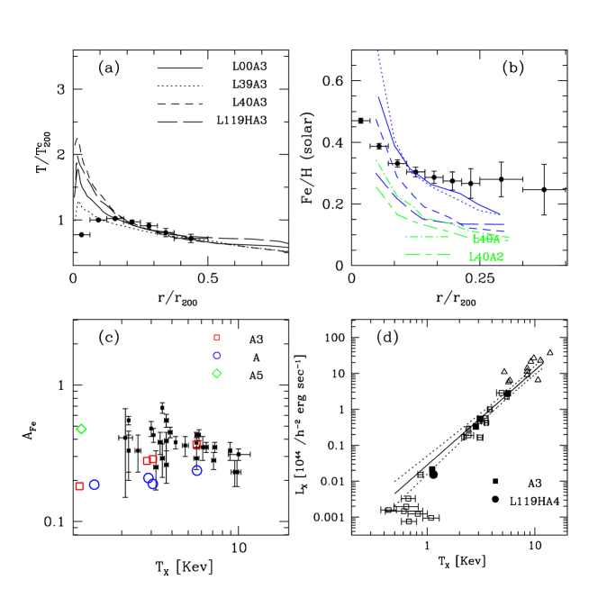
Figure 5: Comparison against data of several observational variables at $z=0$ from the runs with an Arimoto-Yoshi IMF (A). (a): The projected emission weighted temperature profiles as a function of $r/r_{200}$ for the runs A3 (Table 4); data points from De Grandi & Molendi (2002), $T^{c}_{200}$ is $T_{200}$ normalized to match the last data point ($T_{200}\simeq 80\%T^{c}_{200}$). (b): As in panel (a), but for the projected metallicity profiles; data points from the CF clusters of De Grandi & Molendi (2001). Blue lines are the profiles corresponding to the runs of panel (a). (c): Average iron abundances at $r=0.5h^{-1}Mpc$, open squares refer to A3 runs and open circles to A runs; filled squares from the nearby cluster sample of Matsumoto et al. (2000). (d): Bolometric X-ray luminosities as a function of the temperature. Data points from Fig.11 of Tozzi & Norman (2001). For the sake of clarity only a fraction of the data set has been plotted. The continuous line is the best-fit $L_{X}=3.11\cdot 10^{44}h^{-2}(T/6keV)^{2.64}$ of Markevitch (1998), dashed lines are the $68\%$ confidence intervals. Filled squares are the values of $L_{X}$ for the A3 runs, the filled circle refers to the A4 run ($\varepsilon_{SN}=10^{50}erg$). As in Markevitch, $L_{X}$ for the simulated clusters has been estimated by removing a region of radius $50h^{-1}Kpc$ centered on the peak of the gas density. Mass-weighted temperatures have been used as estimators of the spectral-fit temperatures.

The flatness of the observed profiles suggest that at, early epochs, a series of merger events has erased the existing metallicity gradients. Accordingly, the metal abundances from SNII do not show significant spatial gradients, while the iron abundance gradient can be attributed to SNIa [Dupke & White 2000b]. In this scenarios the metal excess distribution is an indicator of the optical light distribution of early type galaxy, as it has been at least partially confirmed by De Grandi & Molendi (2001). This is not the behavior of the simulated cluster sample. Fig. 3 shows for two clusters the iron radial distribution originated from both SNII and Ia. The iron distributions are very similar, because the timescales of metal ejection is much higher for SNIa than for SNII this is indicative that the dynamical evolution of the two clusters has been very smooth. As already stressed, this cluster sample has been chosen for the regularity of its members. In order to asses in a significant way the effects of dynamical evolution on the shape of the metallicity profiles it is necessary to perform a statistical analysis over a large (say $\lower 2.15277pt\hbox{$\;\buildrel>\over{\sim}\;$}40$) cluster sample. This task is left to a future paper, where a number of issues will be investigated with a statistically robust cluster sample. For the sake of clarity in panel (b) are also shown the profiles of the runs L40A and L40A2, to be compared with that of L40A3. These profiles are clearly below the measured values and confirm the parameters of model A3 as the ones yielding the best agreement with data.

The iron profile of L119A3 is inconsistent with the data points; the iron abundances are smaller at all the radii. The profile is very similar to the ones of L40A2 and L40A. This is a failure of model A3 that is hard to reconcile within the framework of the adopted prescriptions, unless the diffusion of metals in the ICM is characterized by a minimum diffusion length. The most important difference of $\Lambda$CDM119 is that this is the coldest of the four test clusters, with a mass-weighted temperature of $\sim 1keV$. For this cluster a proper comparison of the simulated iron profiles with the mean metallicity profile of the sample is not possible. The averaged profile is that of 9 cooling flow clusters, with minimum temperatures $\lower 2.15277pt\hbox{$\;\buildrel>\over{\sim}\;$}4keV$. Without measured profiles for cool clusters is therefore difficult to put observational constraints on different model parameters from the simulated profiles.

Figure 6: The final profiles of the simulations L119A3 and L119A4 are compared against those of the corresponding high-resolution runs (thick lines). (a): radial temperature profiles. (b) : Gas density profiles, the profiles with $\rho(0)/\rho_{c}\lower 2.15277pt\hbox{$\;\buildrel<\over{\sim}\;$}10^{2}$ are those of the gas metallicity. (c) : SF rates versus age. (d): Iron abundance profiles.

Global values, $A_{Fe}=M_{Fe}/M_{H}$, of the iron abundances for the simulated clusters are compared in panel (c) for models A and A3 against the estimated values for the nearby cluster sample of Matsumoto et al. (2000) sample. These values have been taken from column 4 of Table 1 of the Matsumoto et al. paper and are estimated at a radius of $0.5h^{-1}Mpc$. For model A3 there is a fair agreement with data, while model A yields values of $A_{Fe}$ which are marginally consistent with the allowed uncertainties ( $90\%$ c.l.). The run L119HA3 has a value $A_{Fe}\simeq 0.2$, about a factor $\sim$ two smaller than that expected extrapolating the sample average below the minimum ($\simeq 2keV$ ) cluster sample temperature. This is connected with the results shown in the previous panel. Without a minimum smoothing length there is a clear tendency in the simulations to produce a lesser amount of iron than that inferred from observations for cool clusters.

The open diamond of Fig. 5(c) is the value of $A_{Fe}$ ( $\sim 0.47$, see Table 5) for the run L119HA5. For this simulation, a minimum value $h_{min}^{s}=12Kpc$ has been assumed for the smoothing length of metals in the ICM. Such a high value of $A_{Fe}$ is clearly more indicated to account for the iron abundance of low temperature clusters. The observational evidence of an iron abundance decreasing with $T_{X}$ is however statistically weak [Mushotzky & Lowenstein 1997, Finoguenov, Arnaud & David 2001]. Furthermore, an increase of $A_{Fe}$ for cool clusters can be an artifact due to the presence of a dominant galaxy in the cluster central region. For example, Fukazawa et al. (2000) have removed the contribution of the central region for those clusters with a cD galaxy and for their cluster sample found that there is not a significant correlation $A_{Fe}-kT_{X}$. This is also in agreement with what was found by Finoguenov et al. (2001). A statistical comparison between the $A_{Fe}$ distribution generated by the simulations and the one from real data has been performed for the models discussed above. The statistical tests applied to the $A_{Fe}$  data and the $A_{Fe}$  distribution of the simulated cluster sample are the Student t-test for the means, the F-test for the variances and the Kolgomorov-Smirnov (KS) test for the distributions. The corresponding probabilities give the significance level that, according to the analyzed quantities, the two sets are originated from the same process. The results are presented in Table 6. Model A is clearly ruled out, model A3 is marginally consistent. This is because the value $A_{Fe}$ of L119HA3 is significative to lower the mean of the sample. A much better agreement is obtained if the global iron abundance is given by the run L119HA5 for the cluster $\Lambda$CDM119.

Finally, the final values of the bolometric X-ray luminosity are shown in panel (d) as a function of the cluster temperature. Mass-weighted temperature have been used as unbiased estimators of the spectral temperatures [Mathiesen & Evrard 2001]. The luminosity $L_{X}$ of the simulated clusters is calculated as described in sect. 2. Data points are those of Fig. 11 of Tozzi & Norman (2001). For the sake of clarity, not all the points of the Figure are plotted in the panel. For a consistent comparison with data, a central region of size $50h^{-1}Kpc$ has been excised [Markevitch 1998] in order to remove the contribution to $L_{X}$ of the cooling flow central region. For model A3, the $L_{X}$ of the simulations are in excellent agreement with data over the entire range of temperatures. An additional run has been performed for the cluster with the lowest temperature ($\Lambda$CDM119). The parameters of this run (A4) are the same of model A3, expect for a SN feedback energy of $10^{50}$ erg being used for both SNII and Ia. This value is $10\%$ of that of model A3 and has been considered in order to investigate the effects on final X-ray properties of the amount of heating returned to the ICM by SNe. As can be seen, for model A4 the final $L_{X}$ of the run L119HA4 is very similar to that of L119HA3. The result demonstrates that final X-ray luminosities of the simulations are not sensitive to the amount of SN feedback energy that has heated the ICM. In fact, a simulation run with a zero SN energy returned to the ICM ($\varepsilon_{SN}=0$) yields very similar results. These results are particularly relevant in connection with the recent proposal [Bryan 2000] that the X-ray properties of the ICM are driven by the efficiency of galaxy formation, rather than by heating due to non-gravitational processes. Final profiles for models A3 and A4 are investigated in more detail in Fig. 6 and 7.

data-model	$p_{t}$	$p_{F}$	$p_{KS}$
$A_{Fe}$-A	.003	.032	.001
$A_{Fe}$-A3	.082	.694	.120
$A_{Fe}$-A3(5)a	.689	.993	.756
$f_{gas}(500)$-A3	.02	.565	.018
$f_{gas}(200)$-A3	.001	.221	.001
$f_{gas}(500)$-A3(19)b	.143	0.849	0.163

Table 6: Statistical tests applied to distributions obtained from real data and simulated clusters. $p_{t}$ is the Student t–test applied to the means, $p_{F}$ is the F–test for variances and $p_{KS}$ is the KS statistic to discriminate two distributions. $A_{Fe}$ is the measured iron abundances distribution of Fig. 5, panel (c). $f_{gas}$ refers to the observational sample of the two top panels of Fig. 8. The parameters of the model are indicated in Table 4. For the simulated cluster sample the numerical resolution of the runs is L00, L39, L40 and L119H. ^a: This sample has L119HA5 in place of L119HA3. ^b: This sample has only three clusters, but their initial conditions have been set with $\Omega_{b}h^{2}=0.019$.

4.4 SN heating of the ICM and cooled gas fractions

In Fig. 6, the final profiles of the runs L119A3 and L119A4 are compared against those of L119HA3 and L119HA4. The main differences are between the profiles of the standard resolution run and the high-resolution run. The profiles of the runs for the models A3 and A4 are very similar, with the only important difference between the two models being the SFR at early redshifts. The temperature profiles are almost identical, so energy feedback from SNe is not relevant to determine final gas properties. This conclusion is also supported from the entropy profiles of Fig. 7.

In Fig. 7, final distributions of the two runs L119HA3 and L119HA4 are compared. In panel (a) are plotted the Si abundances synthesized in the explosions of SNII and SNIa. There are not large differences between the corresponding profiles. The Si abundances of SNIa are almost identical. For SNII, the Si abundances profile of L119HA4 is higher than that of L119HA3 in the cluster central region ($\lower 2.15277pt\hbox{$\;\buildrel<\over{\sim}\;$}0.1Mpc$). These differences follow because the run L119HA4 has at early redshifts a higher SFR than that of L119HA3 (see also Fig. 6c). This is a consequence of the reduced thermal pressure and higher gas densities in the former simulation. This effect is not relevant for the SNIa explosions because the involved timescales are much higher than those of the early generations of SNII.

The cumulative injected energy per baryon within the radius $r$ is defined as the ratio $E_{SN}(<r)\mu m_{p}/M_{g}(<r)$, where $E_{SN}(<r)$ is the total SN energy injected within that radius, $M_{g}(<r)$ is the corresponding gas mass. This ratio is shown in panel (d) for the two runs. The ratio has a radially decreasing behavior, for the run L119HA3 drops from $\sim 1keV/part$ at $r\simeq 0.1Mpc$ to $\simeq 0.5keV/part$ at $r\simeq 1Mpc\simeq r_{200}$. There is a small drop in the cluster inner region, presumably due to a biased estimate because of the small number of simulation particles for $r\lower 2.15277pt\hbox{$\;\buildrel<\over{\sim}\;$}40Kpc$. For the run L119HA4 the energy per particle ratio has a shape similar to that of the corresponding ratio for the run L119HA3, at $r\sim 1Mpc$ takes the value of $\sim 0.04keV/part$, which is about $\sim 10\%$ of the value of the parent run with $\varepsilon_{SN}=10^{51}erg$. The binned distribution (panel c) is much more noisy than the cumulative one, but it qualitatively confirms the expected behavior.

In order to assess the amount of heating from the SNe, this ratio is often inferred from the measured abundance of metals [Finoguenov, Arnaud & David 2001]. Si abundances are particularly useful because of the similar yields for different SN types. The ratio estimated from the amount of Si abundance $A_{Si}$ is $\varepsilon_{SN}A_{Si}\mu m_{p}/y_{Si}$ with $y_{Si}\sim 0.12$ being the average SN yield of Si. The estimated ratio (thin lines) is in good agreement at all the radii with the values obtained from the simulation. For $\varepsilon_{SN}=10^{51}erg$ the average energy per particle of the cluster $\Lambda$CDM119 is then $\sim 0.5keV/part$ at the virial radius ($r_{200}\sim 1Mpc$). This cluster has a virial temperature $\sim 1.5keV$, from a sample of 18 relaxed clusters with temperature below $\sim 4keV$. Finoguenov, Arnaud & David (2001, see Fig. 9) find an average SN injected energy of $\sim 0.5keV/part$ for a cluster with a temperature $\sim 1keV$. There is therefore a good agreement between the measured amount of thermal energy per particle associated with SN feedback and that predicted by the simulations with the model parameters of Fig. 7.

Figure 7: For the cluster $\Lambda$CDM119 final distributions of the run L119HA3 are compared against those of L119HA4 ($\varepsilon_{SN}=10^{50}erg$). Panel (a) shows the Si abundance of the gas, originated from both SNII and SNIa metal enrichment of the ICM. (b): Entropy profiles $S=T(r)/n_{e}(r)^{2/3}$, where $n_{e}=\rho_{g}(r)/\mu_{e}m_{p}$ and $\mu_{e}\simeq 1.14$. (c): Distribution of the gas particle energy injected by SNe. (d): As in panel (c), but for the cumulative distribution $E_{SN}(<r)/N_{p}(<r)$, where $N_{p}=M_{g}(<r)/\mu m_{p}$. Thin lines correspond to $E_{SN}(<r)/N_{p}(<r)$ as obtained from Si abundance.

The gas entropy is defined as $S(r)=k_{B}T(r)/n_{e}(r)^{2/3}$, where $n_{e}$ is the electron number density. For the two runs L119HA3 and L119HA4 the entropy profiles in units of $keVcm^{2}$ are plotted in panel (b) of Fig. 7. An important result that follows from the radial dependence of the two profiles is that they are almost identical. A simulation with a zero SN energy yields a very similar profile. This means that final ICM properties are largely unaffected by the amount of energy injected by SNe into the ICM. This follows because most of the energy is injected in the cluster central region where the gas density is higher and cooling is very efficient to radiate away the energy of the reheated gas. Energy feedback from SNe can modify the ICM state for small clusters or groups with $T_{X}\lower 2.15277pt\hbox{$\;\buildrel<\over{\sim}\;$}1keV$. Another important result from the entropy profiles of Fig. 7 is the entropy level of the gas at $r\sim 0.1R_{V}\simeq 0.1r_{200}\simeq 0.1Mpc$. At this radial distance the gas entropy of the simulated cluster is $\sim 200keVcm^{2}$, a value consistent with a set of observations [Ponman, Cannon & Navarro 1999, Lloyd–Davies, Ponman & Cannon 2000, Wu & Xue 2002a] for a system with $T_{X}\sim 1.5keV$. Together with the good agreement between the $L_{X}-T_{X}$ relation obtained from simulations with that from observations these findings provide strong support for the radiative cooling model proposed by Bryan (2000).

According to this scenario [Bryan 2000, Voit & Bryan 2001, Wu & Xue 2002a, Muanwong et al. 2002, Davé et al. 2002] the efficiency of galaxy formation is higher in groups and cool clusters than in hot clusters. The low-entropy cooled gas is removed because of galaxy formation, and is replaced by the inflow of the surrounding high-entropy gas. The higher efficiency of galaxy formation for cool systems explains the central entropy excess over the self-similar predictions [Ponman, Cannon & Navarro 1999]. One of the most important observational consequences of the cooling model is that the fraction of hot gas $f_{g}=M_{g}/M_{T}$ increases going from cool clusters to hot clusters. Conversely, the fraction $f_{star}$ of cooled gas turned into stars should decrease with the mass of the system.

Observational evidence for a dependence of $f_{g}$ with $T_{X}$ is controversial [David et al. 1990, David, Jones & Forman, Mohr, Mathiesen & Evrard 1999, Arnaud & Evrard 1999, Roussel, Sadat & Blanchard 2000, Balogh et al. 2001]. The main difficulty is the extrapolation to virial radii of the X-ray data for cool clusters, which can bias the estimates of the cooled gas fraction. According to Roussell et al. (2000) there is not strong observational support for an increase of $f_{gas}$ with $T_{X}$. This is in disagreement with the findings of David, Jones & Forman (1995), who show that the gas fraction $f_{gas}$ increases with the X-ray temperature. According to Mohr, Mathiesen & Evrard (1999) there is a weak dependence of $f_{gas}$ with $T_{X}$ in their X-ray ROSAT sample of 45 galaxy clusters. A constant $f_{gas}$ is inconsistent with the data at $95\%$ confidence level.

Arnoud & Evrard (1999) have analyzed the temperature dependency of $f_{gas}$ for a sample of 24 clusters with accurate measured temperatures and low cooling flows. They have determined $f_{gas}$ for two radii enclosing gas overdensities $\delta=500$ and $\delta=200$. Total masses have been estimated according to two different methods. The $\beta$-model (BM) assumes an isothermal gas density profile in hydrostatic equilibrium with the shape determined according to the X-ray surface brightness. The virial theorem (VT) estimates the cluster total mass according to virial equilibrium at a fixed density contrast. The relation is calibrated from a set of numerical experiments [Evrard, Metzler & Navarro 1996] and is not sensitive to the assumed cosmological model. According to Arnaud & Evrard (1999) it is difficult to draw conclusions on the dependence of $f_{gas}$ on the cluster temperature. The results depend on the chosen model. For the BM model, the difference in the value of $f_{gas}$ between subsamples of cool clusters and hot ($>4keV$) clusters is not statistically significant. For the VT model this difference is at the $3\sigma$ level at a radius corresponding to a gas overdensity $\delta=500$. Arnaud & Evrard (1999) indicate a conservative upper limit of $\sim 30\%$ in the $1\sigma$ fractional error of $f_{gas}$.

For the cluster sample of Arnaud & Evrard (1999), the gas fraction $f_{gas}$ is shown as a function of the total cluster mass in the top panels of Fig. 8. The sample distributions are derived from the VT model at a density contrast of $\delta=500$ (top left panel) and $\delta=200$ (top right panel). The data points are those in the top panels of Fig. 3 of Arnaud & Evrard (1999), with an assumed $\simeq 30\%$ uncertainty. (top right panel). For the model A3 the corresponding values of $f_{gas}$ at $\delta=500$ and $\delta=200$ from the numerical cluster sample are also shown as open squares. There is a clear tendency for the two simulated cluster distributions to follow the $f_{gas}$ distribution of the data, but with a reduced amplitude. The result of a statistical comparison are reported in Table 6. The $f_{gas}$ distribution of model A3 at $\delta=500$ is inconsistent with data with a high significance level ($95\%$ c.l.), and the situation at $\delta=200$ is even worse. For this overdensity, an extrapolation of X-ray data up to the required radius has been performed [Arnaud & Evrard 1999] in order to evaluate the corresponding data points. Therefore, possible biases can undermine the estimate of $f_{gas}$ at $\delta=200$. For $f_{gas}[\delta=500]$ a possible source of disagreement between the numerical distribution and that of data points lies in the assumed value of the cosmological baryonic density $\Omega_{b}$ in the simulations. Here it has been assumed $\Omega_{b}h^{2}=0.015$, but recent measurements [Burles & Tytler 1998] favor $\Omega_{b}h^{2}=0.019$. In correspondence to this value of $\Omega_{b}$ in the initial conditions of the simulations, the values of $f_{gas}[\delta=500]$ are displayed in Fig. 8(a) for a subsample of three simulated cluster ($\Lambda$CDM00, $\Lambda$CDM119 and a new cluster with virial mass $\sim 2.5\cdot 10^{14}h^{-1}M_{\odot}$). The distribution is now in a better agreement with the data, and the confidence levels for rejecting the null hypothesis are now below $95\%$. Therefore it is fair to say that the ICM gas fractions obtained here are consistent with available observational estimates.

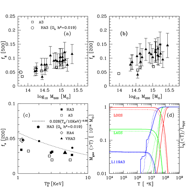
Figure 8: Top panels: gas fraction $f_{g}=M_{g}(<r)/M_{T}(<r)$ versus $M_{T}$ within the radius within which $\rho/\rho_{c}=\delta$, (a) is for $\delta=500$ and (b) is for $\delta=200$. Data points from Fig. 3 of Arnaud & Evrard (1999, VT model). The open circles in panel (a) are the values of $f_{g}$ for runs with $\Omega_{b}=0.019h^{-2}$. (c) : The ratio of the mass of cold gas turned into stars to the total mass is shown as a function of the cluster temperature. The dashed line is the Bryan (2000) best-fit $f_{star}$ to data, rescaled by the factor $f_{baryon}(here)/f_{baryon}(Bryan)=0.1/0.16$. (d): From the left, gas mass above a given temperature $T$ is plotted as a function of the temperature itself. Dashed lines are for the very-high resolution runs VH, while L119HA3 is for $\Lambda$CDM119. From the right: the fraction of total X-ray luminosity that is emitted from the gas below a given temperature is shown for the runs corresponding to the gas masses on the left.

The predictions of the radiative cooling model for the ICM evolution have been recently investigated in a number of papers, either through analytical methods [Bryan 2000, Voit & Bryan 2001, Wu & Xue 2002a, Voit et al. 2002, Wu & Xue 2002b] or with numerical simulations [Muanwong et al. 2001, Muanwong et al. 2002, Davé et al. 2002]. Results from the employed methods clearly show a decreasing $f_{star}$ with the cluster temperature. The dependence of $f_{star}[\delta=200]$ on $T_{X}$ is shown in Fig. 8(c) for the four test clusters. Open squares are for model A3 with standard resolution and filled squares refers to the high-resolution runs. For comparative purposes the $f_{star}$ predicted by the analytical model of Bryan (2000) is also shown. Because of the different values of $\Omega_{b}$ and $\Omega_{m}$ in the paper of Bryan, $f_{star}$ has been approximately rescaled by the factor $f_{b}(here)/f_{b}(Bryan)=0.1/0.16=0.625$. There is a fair agreement of the model with the simulations at high temperatures, but for $T_{X}\sim 1keV$ $f_{star}$ of the simulations is below the model predictions by a factor $\sim$ two. The disagreement at low temperatures is ameliorated for the runs with $\Omega_{b}h^{2}=0.019$, in such a case $f_{star}(Bryan)$ must be rescaled by the factor $\sim 0.81$. The predicted value of $f_{star}$ is now $\sim 0.075$ at $T_{X}\simeq 1keV$, which is a factor $\simeq 50\%$ higher than the value $\sim 0.05$ of $f_{star}$ at the same temperature for the runs with $\Omega_{b}h^{2}=0.019$.

The comparison of $f_{star}$ with data is a controversial issue [Balogh et al. 2001], also because of the lack of firm bounds on the allowed uncertainties [Roussel, Sadat & Blanchard 2000]; however, it is worth stressing that Roussel et al. (2000) found a weak dependence of the gas fraction on cluster temperature when the estimates of virial masses are calibrated from numerical simulations rather than inferred from the $\beta$-model. The dependence is not statistically significant because of the large size of the sample error bars. A comparison of $f_{star}$ predicted by an analytical model has been performed by Wu & Xue (2002b) against the Roussell et al. (2000) data. The theoretical predictions are of about twice as high as the sample values. From Fig. 8(c) the values of $f_{star}[\delta=200]$ for the three runs with $\Omega_{b}h^{2}=0.019$ can be compared with the analytical predictions of the Wu & Xue (2002b) model (cf. Fig. 2 of their paper). The values of $\Omega_{b}$ and $h$ are slightly different, but there is a broad agreement. At $T_{X}\sim 1keV$ $f_{star}(here)\simeq 0.05$ is lower than the theoretically predicted value $\simeq 0.07$. As noted by Wu & Xue theoretical models of cooling yield a dependence of $f_{star}$ on $T_{X}$ steeper than that found in hydrodynamical simulations and observations. At low temperatures $f_{star}$ of the simulations is in better agreement with the Rousell at al. (2000) data, but the observed uncertainties do not allow firm conclusions. The simulations results for $f_{star}$ are also in qualitative agreement with those of the radiative model of Muanwong et al. (2002). In units of $\Omega_{b}/\Omega_{m}$ the values of $f_{star}(f_{g})$ range from $\sim 0.38(0.46)$ from $M_{200}=0.8\cdot 10^{14}h^{-1}M_{\odot}$ to $\sim 0.34(0.56)$ for a cluster with a virial mass of $M_{200}\sim 2.4\cdot 10^{14}h^{-1}M_{\odot}$. These values are not very different from those which can be inferred from the distributions plotted in Fig. 3(b) on Muanwong et al. (2002) for their radiative model. The cosmological parameters of the simulations of Muanwong et al. (2002) are identical to those assumed here ($\Omega_{m}$ is a $\sim 20\%$ higher), and the numerical resolution is broadly similar.

Finally, the effects of the numerical resolution on the predicted final amount of cooled gas are shown in panel (d) of Fig. 8. As a function of the gas temperature the fractional contribution to the total X-ray luminosity is plotted from the right for runs of three clusters ($\Lambda$CDM00, $\Lambda$CDM40 and $\Lambda$CDM119) with different resolutions. For the first two clusters the ratio of $L_{X}(<T)/L_{T}$ for very high-resolution runs are compared against that of standard resolution. The ratio $L_{X}(<T)/L_{T}$ of the run L119A3 is instead compared against that of L119HA3. From the left, the gas masses above a given gas temperature are plotted for the corresponding runs. The distribution of the gas mass versus the gas temperature shows that resolution effects are most important in the low-temperature region of the gas temperature distribution, whereas X-ray luminosities are largely determined by the high-temperature part of the distribution. This demonstrates that the fraction of cold gas depends on the numerical resolution, as can be seen from Fig. 8(c), but is not a source of concern as far as X-ray properties are interested.

For the cluster $\Lambda$CDM119, the quantity, $M_{gas}(>T)$ is weakly dependent on the numerical resolution of the simulations. From Fig. 8(c), one can see that $f_{star}$ at low temperatures also seems to converge as the resolution is increased. This issue is strictly related to the global value of the baryonic fraction of cooled gas $\Omega_{cold}/\Omega_{b}=f_{b}(global)$. Observational upper limits indicate $f_{b}(global)\lower 2.15277pt\hbox{$\;\buildrel<\over{\sim}\;$}10\%$ [Balogh et al. 2001]. According to Balogh et al. (2001), the global fraction $f_{b}(global)$ is expected to increase as the resolution limit of the simulation is increased, unless a feedback model is incorporated in the simulation. The results of the high-resolution runs suggest that at low temperatures convergence is being achieved for $f_{star}$ and that the feedback model implemented here effectively regulates the amount of cooled gas. This is strongly indicated by the large value of $f_{star}$ ($\sim 0.05$) when the SN feedback energy is reduced (open diamond of Fig. 8(c), which corresponds to the run L119HA4). For clusters with temperatures above $\lower 2.15277pt\hbox{$\;\buildrel>\over{\sim}\;$}2keV$, the values of $f_{star}$ appear to converge for simulations with a number of gas particles $N_{g}\lower 2.15277pt\hbox{$\;\buildrel>\over{\sim}\;$}200,000$. This is shown in Fig. 8(c), where for the cluster $\Lambda$CDM00 the value of $f_{star}$ for the very-high resolution run L00VHA3 (filled triangle) is $\sim 0.03$ and is close to that of $f_{star}$ for L00HA3. Note that the mass of the gas particle for the run L00VHA3 is only a $\sim 10\%$ higher than that of L119HA3 ($\simeq 7\cdot 10^{8}M_{\odot}$). These issues can be clarified in deeper details with a set of cosmological simulations with different resolutions that incorporate the SN feedback scheme implemented here. Such analysis is beyond the scope of this paper and will be considered in a future work.

5 SUMMARY AND CONCLUSIONS

In this paper results from a large set of hydrodynamical SPH simulations of galaxy clusters have been used to investigate the dependence of iron abundances and heating of the ICM on a number of model parameters. The simulations have been performed with different numerical resolutions and a numerical cluster sample covering nearly a decade in cluster mass. The modeling of the gas physical processes in the simulations incorporates radiative cooling, star formation and energy feedback. The gas is metal enriched from SN ejecta of type II and Ia, and the cooling rate depends on the local gas metallicity. This allows us to follow self-consistently the ICM evolution also for cool clusters, whose departures of cluster scaling relations from self-similarity are most important.

The metal enrichment of the ICM is governed by a number of model parameters. Theoretical uncertainties on the shape of the IMF and nucleosynthesis stellar yields lead to final iron abundances which can differ by a factor $\sim$ two. These two parameters have then been kept fixed for a large fraction of the performed simulations. This is done in order to restrict the full range of the parameter space. They have been chosen so that the corresponding final amounts of iron in the ICM are the ones that most closely agree with that indicated by observations. The ejected metals are distributed among gas neighbors according to the SPH formalism. Final iron abundances have been found to be sensitive to the shape of the smoothing kernel of the ejected metals $W_{Z}$ and to the constraints on the corresponding smoothing lengths $h^{s}$. For a certain choice of the above parameters, it has been found a fair agreement between the observed radial metallicity profiles with those obtained from the simulated clusters. Global iron abundances are also consistent with measured values. There are however a number of issues which are still open.

i) For cool clusters the ejection parameters are not well determined because of the lack of measured iron profiles, also constraints from global iron abundances suffer from selection biases in the cluster samples. The simulated profiles have a radial decay steeper than observed. This difference could be mainly due to the lack in the simulated cluster sample of mergers which have efficiently remixed the metal content of the ICM. The small size of the numerical cluster sample does not allow to reach firm conclusions. In order to investigate the correlation between the shape of the final metallicity profiles with the cluster dynamical evolution it is then necessary to analyze simulation results from a statistically robust (say $\lower 2.15277pt\hbox{$\;\buildrel>\over{\sim}\;$}40$) cluster sample.

ii) A discrepancy with observations is given by the radial behavior of the projected emission-weighted temperature profiles, which have a steep rise at $r\lower 2.15277pt\hbox{$\;\buildrel<\over{\sim}\;$}0.1r_{200}$. This feature is not shared by observations, for the innermost bin the simulated temperatures are higher by a factor $\sim$ two than the measured values. This difference cannot be easily accommodated by the gas physical modeling of the simulations. Because of radiative cooling, an increase of the gas temperature toward the cluster centre is expected as a consequence of entropy conservation [Wu & Xue 2002a]. A certain amount of cooled gas is present in the core of the clusters and is responsible of the strong decline of the temperature profiles at distances very close to the cluster centres ($r\lower 2.15277pt\hbox{$\;\buildrel<\over{\sim}\;$}0.02r_{200}$). This feature could help to reconcile the differences with the shapes of the observed profiles. As found by Mathiesen and Evrard (2001), the measured spectral fit temperatures can be biased toward lower values because of line cooling. An X-ray spectral fit analysis is then necessary to resolve the discrepancies between the simulated and measured temperatures profiles in the cluster core regions.

The ICM X-ray properties of cool clusters are largely unaffected by the amount of feedback energy injected by SNe, with the luminosity-temperature relation being in excellent agreement with data. The final gas entropy distribution has been found almost independent on the heating efficiency, for $T_{X}\sim 1keV$ the core entropy excess is in agreement with estimated values. These findings support the radiative cooling model of Bryan (2000), where the ICM X-ray scaling relations are driven by the efficiency of galaxy formation. The model predicts that at the cluster virial radius the fraction of hot gas $f_{g}$ is positively correlated with the cluster temperature $T_{X}$. A number of observational uncertainties prevents to put tight constraints, but the $f_{g}-T_{X}$ distribution of the simulated cluster sample is not inconsistent with available estimates from X-ray data.

To explain the steepness of the luminosity-temperature relation an alternative to the cooling model is the preheating scenario, where the gas has been heated by an energy injection that occurred at early epochs. Simulation results [Bialek, Evrard & Mohr 2001, Muanwong et al. 2002, Borgani et al. 2002] show that a number of observed X-ray properties can be reproduced in the preheating model. Future X-ray observations of cool clusters and groups with Chandra will help to discriminate between the two models. It is worth noting that simulations of galaxy clusters in the preheating scenario must also include radiative cooling and SN feedbacks. Therefore, the agreement with observations of X-ray properties reproduced here by the simulated clusters in the cooling model suggests that additional heat sources, if required, are most likely to affect the ICM properties of systems with temperatures below $\lower 2.15277pt\hbox{$\;\buildrel<\over{\sim}\;$}1keV$.

References

- [Aguirre et al. 2001] Aguirre A., Hernquist L., Schaye J., Katz N., Weinberg, D.H., Garner J., 2001, ApJ, 561, 521
- [Allen & Fabian 1998] Allen S. W., Fabian A. C., 1998, MNRAS, 297, L57
- [Anninos & Norman 1996] Anninos P., Norman M. L., 1996, ApJ, 459, 12
- [Arimoto & Yoshii 1987] Arimoto N., Yoshii Y., 1987, A&A, 173, 23
- [Arnaud et al. 1992] Arnaud M., Rothenflug R., Boulade O., Vigroux L. & Vangioni-Flam, 1992, A&A, 254, 49
- [Arnaud & Evrard 1999] Arnaud M., Evrard A. E., 1999, MNRAS, 305, 631
- [Bahcall & Fan 1998] Bahcall N. A., Fan X., 1998, ApJ, 504, 1
- [Balogh, Babul & Patton 1999] Balogh M., Babul A., Patton D., 1999, MNRAS, 307, 463
- [Balogh et al. 2001] Balogh M. L., Pearce F. R., Bower R. G., Kay S. T., 2001, MNRAS, 326, 1228
- [Bialek, Evrard & Mohr 2001] Bialek J. J., Evrard A. E., Mohr J. J., 2001, ApJ, 555, 597
- [Borgani et al. 2002] Borgani S., Governato F., Wadsley J., Menci N., Tozzi P., Quinn T., Stadel J. Lake G., 2002, astro-ph/0205471
- [Bower 1997] Bower R. G., 1997, MNRAS, 288, 355
- [Bryan 2000] Bryan G. L., 2000, ApJ, 544, L1
- [Buonomo et al. 2000] Buonomo F., Carraro G., Chiosi C., Lia C., 2000, MNRAS 312, 371
- [Burles & Tytler 1998] Burles S., Tytler D., 1998, Space Sc. Rev., 84, 65
- [Carraro, Lia & Chiosi 1998] Carraro G., Lia C., Chiosi C., 1998, MNRAS 297, 1021
- [Churches, Nelson & Edmunds 2001] Churches D. K., Nelson, A. H., Edmunds M. G., 2001, MNRAS, 327, 610
- [ Davé et al. 2002] Davé R., Katz N., Weinberg D.H., 2002, astro-ph/0205037
- [David et al. 1990] David L. P., Arnaud K. A., Forman W., Jones C., 1990, ApJ, 356, 32
- [David et al. 1993] David L. P., Slyz A., Jones C., Forman W., Vrtilek S. D., Arnaud K. A., 1993, ApJ, 412, 479
- [David, Jones & Forman] David L., Jones C., Forman W., 1995, ApJ, 445,578
- [De Grandi & Molendi 2001] De Grandi S., Molendi S., 2001, ApJ, 551, 153
- [De Grandi & Molendi 2002] De Grandi S., Molendi S., 2002, ApJ, 567, 163
- [Dupke & White 2000a] Dupke R. A., White R., 2000a, ApJ, 528, 139
- [Dupke & White 2000b] Dupke R. A., White R., 2000b, ApJ, 537, 123
- [Edge et al. 1990] Edge A. C., Stewart G. C., Fabian A. C., Arnaud K. A., 1990, MNRAS, 245, 559
- [Eke, Cole & Frenk 1996] Eke V. R., Cole S., Frenk C. S., 1996, MNRAS, 282, 263
- [Evrard & Henry 1991] Evrard A. E., Henry J. P., 1991, ApJ, 383, 95
- [Evrard, Metzler & Navarro 1996] Evrard A. E., Metzler C. A., Navarro J. F., 1996, ApJ, 469, 494
- [Ezawa et al. 1997] Ezawa H., Fukazawa Y., Makishima K., Ohashi T., Takahara F., Xu H., Yamasaki N.Y., 1997, ApJL, 490, 33
- [Finoguenov, David & Ponman 2000] Finoguenov A., David L. P., Ponman T. J., 2000, ApJ, 544, 188
- [Finoguenov, Arnaud & David 2001] Finoguenov A., Arnaud M., David L. P., 2001, ApJ, 555, 191
- [Fukazawa et al. 1998] Fukazawa Y., Makishima K., Tamura T., Ezawa H., Xu H., Ikebe Y., Kikuchi K., Ohashi T., 1998, PASJ, 50, 187
-
[Fukazawa et al. 2000]
Fukazawa Y., Makishima K., Tamura T., Nakazawa K., Ezawa H.,
Ikebe Y.,
Kikuchi K., Ohashi T., 2000, MNRAS, 313, 21 - [Girardi et al. 1998] Girardi M., Borgani S., Giuricin G., Mardirossian F., Mezzetti M. 1998, ApJ, 506, 45
- [Gibson, Loewenstein & Mushotzky 1997] Gibson B. K., Loewenstein M., Mushotzky R. F., 1997, MNRAS 290, 623
- [Greggio & Renzini 1983] Greggio L., Renzini A., 1983, A&A 118, 217
- [Gunn & Gott 1972 ] Gunn J. E., Gott J. R., 1972, ApJ, 176, 1
- [Henry & Arnoud 1991 ] Henry J. P., Arnoud K. A., 1991, ApJ, 372, 410
- [Henry 1997] Henry J. P., 1997, ApJ, 489, L1
- [Hernquist & Katz 1989] Hernquist L., Katz N., 1989, ApJS, 70, 419
- [Irwin & Bregman 2001] Irwin J. A., Bregman J. N., 2001, ApJ, 546, 150
- [Iwamoto et al. 1999] Iwamoto K., Brachwitz F., Nomoto K. et al., 1999, ApJS 125, 439
- [Kaiser 1986] Kaiser N., 1986, MNRAS, 222, 323
- [Kaiser 1991] Kaiser N., 1991, ApJ, 383, 104
- [Kitayama, Sasaki & Suto 1998] Kitayama T., Sasaki S., Suto Y., 1998, PASJ, 50, 1
- [Kravtsov & Yepes 2000] Kravtsov A. V., Yepes G., 2000, MNRAS, 318, 227
- [Lewis et al. 2000] Lewis G.F., Babul A., Katz N., Quinn T., Hernquist L., Weinberg D. H., 2000, ApJ , 536, 623
- [Lia, Portinari & Carraro 2002] Lia C., Portinari L., Carraro G., 2002, MNRAS, 330, 821
- [Lloyd–Davies, Ponman & Cannon 2000] Lloyd–Davies E. J., Ponman T. J., Cannon D. B., 2000, MNRAS, 315, 689
- [Loewenstein & Mushotzky 1996] Loewenstein M., Mushotzky R., 1996, ApJ, 466, 695
- [Loewenstein 2001] Loewenstein M., 2001, ApJ, 557,573
- [ Mathiesen & Evrard 2001] Mathiesen B., Evrard A. E., 2001, ApJ, 546, 100
- [Matsumoto et al. 2000] Matsumoto H., Tsuru T. G., Fukazawa Y., Hattori M., Davis D. S., 2000, PASJ, 52, 153
- [Metzler & Evrard 1994] Metzler C. A., Evrard A. E., 1994, ApJ, 437, 564
- [Markevitch 1998] Markevitch M., 1998, ApJ, 504, 27
- [Miller & Scalo (1979)] Miller G. E., Scalo F. J. M., 1979, ApJS, 41, 513
- [Mohr, Mathiesen & Evrard 1999] Mohr J. J., Mathiesen, B., Evrard, A. E., 1999, ApJ,517,627
- [Monaghan & Lattanzio 1985] Monaghan J. J., Lattanzio J. C., 1985, A&A, 149, 135
- [Mosconi et al. 2001] Mosconi M. B., Tissera P. B., Lambas D. G., Cora S. A., 2001, MNRAS, 325, 34
- [Muanwong et al. 2001] Muanwong O., Thomas P. A., Kay S. T., Pearce F. R., Couchman, H. M. P. 2001, ApJL, 552 L27
- [Muanwong et al. 2002 ] Muanwong O., Thomas P. A., Kay, S. T., Pearce F. R., 2002, astro-ph/0205137
- [Mushotzky & Lowenstein 1997] Mushotzky R. F., Lowenstein, M., 1997, ApJ, 481 L63
- [ Navarro & White 1993] Navarro J., White, S. D. M., 1993, MNRAS, 265, 271
- [Pearce et al. 2000] Pearce F. R., Thomas P. A., Couchman H. M. P., Edge A. C., 2000, MNRAS 317, 1029
- [Ponman, Cannon & Navarro 1999] Ponman T. J., Cannon D. B., Navarro J. F., 1999, Nature, 397, 135
- [Portinari, Chiosi & Bressan 1998] Portinari L., Chiosi, C., Bressan, A., 1998, A&A 334, 505
- [Press & Schechter 1974 ] Press W. H., Schechter P., 1974, ApJ, 187 , 425
- [Raiteri, Villata & Navarro 1996] Raiteri C. M., Villata M., Navarro J. F., 1996, A&A 315, 105
- [Raymond & Smith 1977] Raymond J. C., Smith B. W., 1977, ApJS, 35, 419
- [Roussel, Sadat & Blanchard 2000] Roussel H., Sadat R., Blanchard, A., 2000, A&A, 361, 429
- [Salpeter 1955] Salpeter E. E., 1955, ApJ, 121, 161
- [Sarazin 1986] Sarazin C. L., 1986, Reviews of Modern Physics, 58, 1
- [Steinmetz & Müller 1994] Steinmetz M., Müller E., 1994, A&A, 281, L97
- [Sutherland & Dopita 1993] Sutherland R. S., Dopita M. A., 1993, ApJ, 88, 253
- [Tantalo, Chiosi & Bressan 1998] Tantalo R., Chiosi C., Bressan A., 1998, A&A, 333, 419
- [Tinsley 1980] Tinsley B. M., 1980, Fund. of Cosmic Phys., 5, 287
- [Tozzi & Norman 2001] Tozzi P., Norman C., 2001, ApJ, 546 63
- [Valageas & Silk 1999] Valageas P., Silk J., 1999, ApJ, 350, 725
- [Valdarnini, Ghizzardi & Bonometto (1999)] Valdarnini R., Ghizzardi S., Bonometto S., 1999, New Astr, 4, 71
- [Valdarnini 2002] Valdarnini R., 2002, ApJ, 567, 741
- [Voit & Bryan 2001] Voit G. M., Bryan G. L., 2001, Nature, 414, 425
- [Voit et al. 2002] Voit G. M., Bryan G. L., Balogh M. L., Bower R. G., 2002, astro-ph/0205240
- [White 1991] White R. E., 1991, ApJ, 367, 69
- [White 2000] White D. A., 2000, MNRAS, 312, 663
- [White, Efstathiou & Frenk 1993] White S. D. M., Efstathiou G., Frenk C. S., 1993, MNRAS, 262, 1023
- [Woosley & Weaver 1986] Woosley S. E., Weaver T. A., 1986, ARAA 24, 205
- [Woosley & Weaver 1995] Woosley S. E., Weaver T. A., 1995, ApJS 101, 181
- [Wu, Fabian & Nulsen 2000] Wu K., Fabian, A., Nulsen, P., 2000, MNRAS, 318, 889
- [Wu & Xue 2002a] Wu X.-P., Xue Y.-J., 2002a, ApJ, 569, 112
- [Wu & Xue 2002b] Wu X.-P., Xue Y.-J., 2002b, ApJL, 572, L19
- [Yoshikawa, Jing & Suto 2000] Yoshikawa K., Jing Y. P., Suto Y., 2000, ApJ, 535, 593