Abstract

This work is related to different questions within cosmology. The principal idea herein is to develop cosmological knowledge making use of the analyses of observational data in order to find the values of the matter density $\Omega_{m}$ and vacuum energy density $\Omega_{\Lambda}$.

Data fitting is carried out using two statistical methods, $\chi^{2}$ and maximum likelihood. The data analysis exhibits that a low density and flat Universe is strongly favoured.

Applying the $\Omega_{m}$ value found for clusters of galaxies, we demonstrate that clusters have very little room for baryonic dark matter. An upper limit to the small but non-negligible sum of baryonic dark matter and galaxy mass can be estimated, requiring the use of special statistics.

A Toroidal Black Hole (TBH) study, in contrast to the Spherical Black Hole (SBH), shows that the TBH can be used as an important tool in explaining AGN phenomena.

Chapter 1 Cosmological Models and Parameters

Measurement of global cosmological parameters is one of the key challenges in current cosmology research. People are interested in knowing in what kind of Universe we live. Only a precise measurement of density parameters can tell us the critical nature of the Universe. The parameters determined from the different observations are strongly model dependent and also contradictory to each other. Resolution of contradiction is another big challenge to the scientist. A lot of interesting discussions is reported in this thesis, based on recent output from the cosmological research.

According to the cosmological principle, the Universe is homogeneous and isotropic. Most of the cosmological models are based on Friedman equations, describing a Universe in expansion or contraction. Einstein sought a solution in which the Universe would be static and eternal because the Universe known at that time comprised only the Milky Way, which clearly was not expanding or contracting. In this Chapter a few models will be discussed that are remarkable in modern cosmology.

This thesis deals with Cosmological Parameters and Black Holes. Gravitational matter $\Omega_{m}$ is composed of baryonic matter, baryonic dark matter and dark matter of unknown composition. The matter density ($\Omega_{m}$), baryonic density ($\Omega_{b}$), Hubble constant ($H_{0}$) and the age of the Universe ($t_{0}$) will also be discussed. A discussion on the cosmological constant ($\Lambda$) and its vacuum energy density ($\Omega_{\Lambda}$) will be presented in the next Chapter. A simple picture of different cosmologies are portrayed in Fig. 1.1. Some aspects of Black Hole physics will be discussed in Chapter 6.

1.1 Einstein’s Model

Modern cosmological models began with Einstein’s static cosmology. Einstein proposed that the gravity is not a force but merely a manifestation of free motion in space-time. In addition, the geometry of space-time is determined by the energy in the Universe. The energy is associated with mass, radiation and pressure. A cosmological constant $\Lambda$ was introduced by Einstein into the equation of General Relativity to allow for a stationary solution, and it was introduced before the concept of Big Bang. However, the idea of a static Universe fails to agree with observations, because the Universe is expanding linearly with time.

1.2 The de Sitter Model

In 1917, Willem de Sitter discovered a cosmological model differing from Einstein’s. He observed that the light from distant objects becomes redder as the distance increases. There is no matter in this model. The space-time is flat, and the space expands exponentially because of the $\Lambda$ force. This is one of the earliest models that was considered when the modern science of cosmology was in its infancy.

1.3 The Einstein-de Sitter Model

According to Einstein and de Sitter, the cosmological constant should be set equal to zero, and they derived a homogeneous and isotropic model. They assumed that the spatial curvature of the Universe is neither positive nor negative but rather zero. The special geometry of the Einstein-de Sitter Universe is Euclidean, but the space-time is not globally flat. People with a philosophical bent have long considered it as the most fitting candidate to describe the actual Universe. Strong theoretical support for this viewpoint came from particle physics, but as yet not definitive, astronomical observations also supported this model.

1.4 The Friedman-Lemaître Model

The standard model of cosmology describes the Universe as expanding at present. The formulation and prediction of a Big Bang expansion for the Universe is remarkable. Both Friedman and Lemaître in different years, independently discovered the solution to Einstein’s equations of gravitation which described an expanding Universe. The expansion could either continue forever, or eventually reverse into a phase of contraction.

However, the Friedman-Lemaître evolutionary model could not predict explicitly the curvature of the expansion, permitting three possible solutions: either hyperbolic, flat or spherical expansion. Friedman’s equations may be written (Kolb & Turner 1990, Roos 1997, Bergstr$\rm\ddot{o}$m & Goober 1999) as

$${\dot{R}^{2}+kc^{2}\over R^{2}}-{\Lambda\over 3}={8\pi G\rho\over 3}$$ (1.1)

$${2\ddot{R}\over R}+{\dot{R}^{2}+kc^{2}\over R^{2}}-\Lambda=-{8\pi Gp\over c^{2}},$$ (1.2)

where R is the scale factor of the Universe, k is the curvature parameter, $\Lambda$ is the cosmological constant, G is the Newtonian constant, $\rho$ is the total energy density and p is the total pressure.

There is a relation between pressure and density, called equation of state

$$p=\alpha\cdot\rho$$ (1.3)

where $\alpha$ is a constant, different in different eras of the Universe. In the radiation dominated era $\rho\sim{1\over R^{4}}$, and in the matter dominated era $\rho\sim{1\over R^{3}}$. For the de Sitter model $\alpha$ = -1, but for interacting fields and topological defects $\alpha$ can vary between -1 and 0. Since recent supernovae observations show that the Universe is accelerating, one has -1 $\leq$ $\alpha$ $<$ -${1\over 3}$. Models with $\alpha$ in this range some people call Quintessence models.

The critical density of the Universe at redshift z is

$$\rho_{c}(z)={3H^{2}(z)\over 8\pi G}$$ (1.4)

where H is the Hubble constant. The vacuum energy density parameter $\Omega_{\Lambda}$ is related to the cosmological constant $\Lambda$ by

$$\Omega_{\Lambda}={\Lambda\over 3H_{0}^{2}}={\rho_{\Lambda}\over\rho_{c}},$$ (1.5)

where the notation zero means the value at present. The matter density parameter of the Universe is

$$\Omega_{m}={\rho_{m}\over\rho_{c}}.$$ (1.6)

The total density parameter of the Universe is the sum of matter density parameter and the vacuum energy density parameter

$$\Omega_{0}=\Omega_{m}+\Omega_{\Lambda}.$$ (1.7)

The flat condition of the Universe is [k = 0 in Eqs. (1.1) and (1.2)]

$$\Omega_{m}+\Omega_{\Lambda}=1$$ (1.8)

We can arrive at a relation among $H_{0},\Omega_{m}$, $\Omega_{\Lambda}$ and $t_{0}$, from the Friedman-Lemaître model, as

$$t_{0}={{1}\over{H_{0}}}\int_{0}^{1}\hbox{d}x\big{[}(1-\Omega_{m}-\Omega_{\Lambda})+\Omega_{m}x^{-1}+\Omega_{\Lambda}x^{2}\big{]}^{-1/2}.$$ (1.9)

This equation will be used to determine the age of the Universe. There is no analytical solution to this integration but it can easily be evaluated numerically. To determine $t_{0}$, we need to have precise values of other parameters. The evaluation of $\Omega_{m}$, $\Omega_{\Lambda}$ can be found in Papers (II), (III), (IV) and also in the next Chapters.

1.5 Density Parameters

Generally, matter density and vacuum energy density are treated as Universal density parameters, and the total matter density is the combination of different kinds of matter. So far as we know, there are two kinds of matter in the Universe, baryonic matter and dark matter. Thus the total mass density parameter $\Omega_{m}$ is the sum of these two. The candidates of dark matter and their nature will be discussed in the Chapter 5. For a long time, the physicists had neglected $\Omega_{\Lambda}$, simply it was considered that $\Omega_{\Lambda}=0$ and $\Omega_{m}=1$. The situation has changed in the last few years by the enormous data collection of powerful telescopes and by the success of satellite missions. Observations suggest that this is not our real Universe.

Due to the expansion of the Universe the mass density is decreasing and the vacuum energy density is now dominating. The vacuum energy is related to the cosmological constant, Eq. (1.5). Most recent measurements agree that the value of present matter density $\Omega_{m}\sim{1\over 3}$ in the flat case. It is the proper time for the astrophysicists and cosmologists to have a direct constraint on the density parameters. The constraints on matter density $\Omega_{m}$ and vacuum energy density $\Omega_{\Lambda}$ are extensively described in the next Chapters.

1.6 Baryonic Density

The value of the universal baryonic density parameter $\Omega_{b}$ follows from standard Big Bang Nucleosynthesis (BBN) arguments, and from the observed abundances of ⁴He, D, ³He, and ⁷Li (cf. eg. Sarkar 1999), in particular from the low deuterium abundance measured by Burles et al. (1999, 2001). Their estimate is

$$\Omega_{b}h^{2}=0.020\pm 0.001\ (68\%\ {\rm CL})$$ (1.10)

where $H_{0}=100h$. Thus, taking this central value and the Hubble constant from Gibson & Brook (2001) we get today’s universal baryonic density $\sim 4\%$. The BBN value is in disagreement with the recent observations of CMB anisotropy which yields (Jaffe et al. 2001)

$$\Omega_{b}h^{2}=0.033_{-0.004}^{+0.005}\ (68\%\ {\rm CL}).$$ (1.11)

Note that BBN provides a probe of the Universal abundance of baryons when the Universe was only a few minutes old. Observations of CMB anisotropy probe the baryon abundance when the Universe was 3-5 hundred thousand years old, and SNe Ia supernovae and clusters of galaxies observations probe a more recent past, when the Universe was several billion years old.

Most recently, the Degree Angular Scale Interferometer (DASI) has measured the angular power spectrum of the Cosmic Microwave Background anisotropy over the range 100 $<$ l $>$ 900 (Pryke et al. 2001). Here, the second peak is more pronounced than found BOOMERANG (de Bernardis et al. 2000) and MAXIMA-1 (Balbi et al. 2000), and the contradiction with BBN can be resolved. DASI (Pryke et al. 2001) gives a new value of baryonic density as

$$\Omega_{b}h^{2}=0.022_{-0.003}^{+0.004}\ (68\%\ {\rm CL}),$$ (1.12)

which is a good agreement with BBN (Burles et al. 2001). DASI has also independently determined $\Omega_{m}=0.40\pm 0.15$ and $\Omega_{\Lambda}=0.60\pm 0.15$ (68% CL), although the errors ber is large and no contour plot is given. Adding the data at higher $l$ BOOMERANG (de Bernardis 2001) has reported the value of $\Omega_{b}h^{2}$, their new value is exactly same as (DASI 2001) Eq. (1.12).

Assuming that the BBN value for $\Omega_{b}h^{2}$ in Eq. (1.10) (Burles et al. 2001) is correct, and taking the value of the Hubble constant $h=0.73\pm 0.05$ Gibson & Brook (2001), one can obtains a constraint on the baryonic density parameters, $\Omega_{b}=0.038\pm 0.002$.

1.7 The Hubble Constant

In 1929, Edwin Hubble discovered that the distant galaxies are moving away from us. A simple mathematical relation between the Hubble constant and distant objects is $H_{0}={v/d}$, where v is the galaxy’s radial velocity and d is the galaxy’s distance from the earth. This is one of the important parameter because it is directly related to the age of the Universe, and it is also related to the other cosmological parameters. The Hubble constant is well determined from the HST Key Project on the Extragalactic Distance Scale (Mould et al. 2000), obtained by the combination of four methods (SBF, FP, Tully-Fisher, and SNe Ia). Their combined result is $H_{0}=71\pm 6{\rm\ km\ s^{-1}Mpc^{-1}}$. A new value of the Hubble constant is presented by Gibson & Brook (2001) performing the re-analysis of the combined Calan-Tololo and Center for Astrophysics (CfA) type SNe Ia datasets. The fit is extremely good with 3% statistical and 10% systematic errors. With a calibration to the corrected Hubble Diagrams by seven high-quality nearby SNe Ia the Hubble constant becomes

$$H_{0}=73\pm 2(r)\pm 7(s)\rm{\ km\ s^{-1}Mpc^{-1}}\ .$$ (1.13)

However, the results agree with each other at $1\sigma$ level. The Hubble constant as measured by different methods summarized in table 1.1

Method	$H_{0}$	Error (%)	References
Type Ia supernovae	73	$\pm{2(r)}\pm{7(s)}$	[45]
Combined HST methods	71	$\pm{2(r)}\pm{6(s)}$	[42]
Tully-Fisher clusters	71	$\pm{3(r)}\pm{7(s)}$	[108]
FP clusters	82	$\pm{6(r)}\pm{9(s)}$	[65]
SBF clusters	70	$\pm{5(r)}\pm{6(s)}$	[40]
Type II supernovae	72	$\pm{9(r)}\pm{7(s)}$	[111]
Cepheids, Metallicity-corrected	68*)	$\pm{5(r\&s)}$	[84]
S-Z effect	66	$\pm{13(r)}\pm{15(s)}$	[77]

Table 1.1: The Hubble constant in units of $\rm{km\ s^{-1}Mpc^{-1}}$. Random (r) and systematic (s) errors are given at 1$\sigma$ confidence level. *) Taking into account more recent calibrations of the LMC distance, this value increases to 74 (cf. eg. Gibson & Brook 2001).

1.8 Age of the Universe

The absolute age of the Universe $t_{0}$ depends on $(h,\Omega_{m},\Omega_{\Lambda})$. The mass density of the Universe $\Omega_{m}$ and the cosmological constant $\Omega_{\Lambda}$ are known from the present analysis. Now we can apply a constraint on $t_{0}$, since our analysis strongly preferred a flat geometry in the Universe and this constraint is valid is the flat case also. In Papers II & III we have determined the age of the Universe to be $t_{0}=13.5\pm 1.3$ (0.68/h) Gyr, where we use the earlier Hubble constant $H_{0}=68\pm 5\ {\rm km\ s^{-1}Mpc^{-1}}$ (Nevalainen & Roos 1998). Since the age of the Universe $t_{0}$ strongly depends on the Hubble constant, our value also changes with Hubble value. Note that the Universe must be older than any other object in the Universe. Our determination agrees well with others as can be seen in table 1.2. The age determination from the different experiments are summarized in table 1.2.

Technique	h Assumption	Age (Gyr)	Objects	References
Stellar ages	None	$13.3\pm{1.1}$	Halo GC	[61]
Stellar ages	None	$12.5\pm{1.5}$	Halo GC	[47]
High-Z	$0.65\pm{0.02}$	$14.2\pm{1.7}$	Universe	[100]
High-Z (flat)	$0.65\pm{0.02}$	$15.2\pm{1.7}$	Universe	[100]
SCP	0.63	$14.2\pm{1.0}$	Universe	[94]
SCP (flat)	0.63	$14.9_{-1.1}^{+1.4}$	Universe	[94]
4-constraints	$0.68\pm{0.10}$	$13.4\pm{1.6}$	Universe	[71]
9-constraints	$0.68\pm{0.05}$	$13.5\pm{1.3}$	Universe	[103]
MCA*)	$0.70\pm{0.15}$	$13.2_{-2.0}^{+3.6}$	Universe	[41]

Table 1.2: Comparison of the age of Universe estimated using different observations. Errors are given at 1$\sigma$ confidence level. *) Multiband Colour Alalysis of bright clusters.

Figure 1.1: Geometry of different types of Universe in $(\Omega_{m},\ \Omega_{\Lambda})$ plane. Flat and open models are infinite; closed models are finite. There are also possibilities that an infinite Universe can collapse if $\Omega_{\Lambda}<0$. A finite Universe expands for ever if $\Omega_{\Lambda}=0$ with $\Omega_{m}\leq 1$, and collapses into a big crunch if $\Omega_{m}>1$. A Finite Universe can be accelerating/decelerating.

Chapter 2 Problem of Missing Energy and Cosmological Constant

2.1 The Cosmological Constant

The cosmological constant is not a constant it might be change with time. It is related to vacuum energy density, Eq. (1.5), and it is a potentially important contributor to the dynamical history of the Universe. The relation between the cosmological constant $\Lambda$ and the vacuum energy density $\Omega_{\Lambda}$ were shown in the previous Chapter. A strong evidence for a non-zero cosmological constant comes from the Supernovae Cosmology Project (SCP), Perlmutter et al. (1999), and the High Redshift Supernovae Search Team (HSST), Riess et al. (1998). In contrast to standard general relativity, a wide theoretical discussion on a non-zero cosmological constant can be found in Carroll & Press (1992), Carroll (2000). We show that three independent constraints strongly rule out the standard model of flat space with vanishing cosmological constant (Fig. 2.2 & Fig.2.3 and for details Paper I). However, the present value of the cosmological constant is an empirical issue, a precise determination of which would be one of the greatest successes of observational cosmology in the near future. If the cosmological constant today comprises most of the energy density of the Universe, the age of the Universe is much older.

The most surprising recent advance in cosmology is that 70% of the Universe seems to be made of vacuum energy. We have combined most recent observational data in the next Chapters to demonstrate this evidence. Our two dimensional maximum likelihood gives a matter density of $\Omega_{m}=\Omega_{dark}+\Omega_{b}=0.31$ and a vacuum energy density of $\Omega_{\Lambda}=0.68$. The total density of the Universe is $\Omega_{0}=\Omega_{m}+\Omega_{\Lambda}=0.99$ (Paper IV).

In figure 2.2 & Fig.2.3 we show our recent (Paper IV) allowed region in ($\Omega_{m},\Omega_{\Lambda}$)-plane. The small solid square and the big dashed square are for the flat and two-dimensional cases indicated, respectively.

Figure 2.1: $\Lambda$ is in the center of physics.

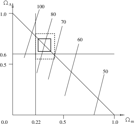
Figure 2.2: Regions allowed in the $(\Omega_{0},\Omega_{\Lambda})$-space. The set of solid lines are imposed by the observation of the radio galaxy 53W091 assuming $\alpha=0$. The numbers indicate the value of the Hubble constant in units of km s^-1 Mpc^-1. The limits $\Omega_{m}<0.22$, $\Omega_{\Lambda}>0.6$ are indicated. The solid and dashed square boxes indicate the recent (Paper IV) allowed region in the parameter space.

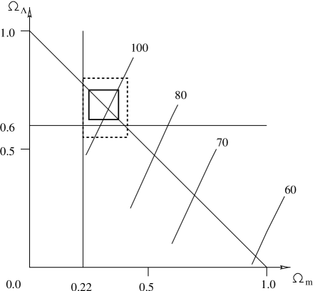
Figure 2.3: As Fig. 2.2, but for $\alpha$ = -0.1

2.2 The Missing Energy Problem

The missing energy may be realized by comparing with the critical energy and the observed energy. Inflationary cosmology and current cosmic microwave anisotropy measurements suggest that the Universe is flat. At the same time observations indicate that the sum of ordinary (baryonic) and dark matter in the Universe is below the critical density. So, the “missing energy” problem arises. It is possible that the missing energy could be from the interacting fields or topological defects (Steinhartz 1996, Huey et al. 1999, Bludman & Roos 2001). As the Universe expands, the missing energy density varies as $(R)^{-3(1+\alpha)}$, where $\alpha=0$ for ordinary matter, $-{1\over 2}\geq\alpha$ $>$ - 1 for quintessence and $\alpha=-1$ for the cosmological constant.

We can write the luminosity distance relation as

$$H_{0}d_{L}=z+{1\over 2}(1-q_{0})z^{2}$$ (2.1)

where

$$q_{0}={1\over 2}\Omega_{m}+({1+3\alpha\over 2})\Omega_{\Lambda},$$ (2.2)

$q_{0}$ is the deceleration parameter, $\alpha$ is the ratio of pressure to energy density of missing energy, and its significance is described in Chapter 1. The deviation of linear law depends on equation of state $\alpha$, the ratio of pressure to energy density of missing energy as seen in Fig. 2.4

Figure 2.4: The luminosity distance versus redshift in different cosmologies. The lower solid line corresponds to $\Omega_{m}=1,\ \Omega_{\Lambda}=0$ and $\alpha=-{1\over 2}\ {\rm or}\ -{2\over 3}$, Einstein-de Sitter, the middle solid line corresponds to $\alpha=-{2\over 3},\ \Omega_{m}=0.31,\ \Omega_{\Lambda}=0.68$, the upper solid line corresponds to $\alpha=-{2\over 3},\ \Omega_{m}=0,\ \Omega_{\Lambda}=1$ de Sitter, the lower and upper dot lines correspond to $\alpha=-{1\over 2},\ \Omega_{m}=0.31,\ \Omega_{\Lambda}=0.68$ and $\alpha=-{1\over 2},\ \Omega_{m}=0,\ \Omega_{\Lambda}=1$ de Sitter respectively. The effects of different models are observable at high redshift rather than at low redshift.

Chapter 3 Observational Constraints

While developing science and technology, astrophysical objects become more visible to us, leading to remarkable developments in cosmology in the last few years. The constraints on cosmological parameters have been published from the analysis of different observational data. The constraints on cosmological parameters differ from one observation to another. Sometimes the conflict is very strong. We partake in resolving this contradiction by paying rigorous attention to statistics, and by combining data from recent observations. In a sequence of Papers I-III we combined all types of data having a published error on $\Omega_{m}$ and $\Omega_{\Lambda}$, using simple $\chi^{2}$ analysis. This, of course, implied believing in the errors and treating them as Gaussian. The techniques and observations usually attributed by the astrophysicist for constraining cosmological parameters are summarized in this Chapter, and the results of our $\chi^{2}$ analysis are discussed.

3.1 Cosmic Microwave Background Radiation

The Cosmic Microwave Background (CMB) is one of the important probes of the early Universe, and it was dramatically discovered in 1965 by Penzias and Wilson. The first result on temperature variations was published by the Cosmic Background Explorer (COBE) satellite (Smoot et al. 1992). The analysis was done in a two-parameter space: the scalar tilt of density fluctuation of the power spectrum $n_{s}$, and the CMB quadrupole normalization Q. The power spectrum $P(k)$ can be written as $P(k)\propto k^{n}$, where $n$ is the tilt of primordial spectrum.

The primary aim of the CMB experiments is to determine the power spectrum, $C_{l}$, of the CMB as a function of multipole moment $l$. Given a map of the temperature $T({\rm\hat{n}})$ in each direction ${\rm\hat{n}}$ on the sky, the power spectrum can be obtained by expanding in spherical harmonics,

$$\left|a_{lm}\right|=\int d{\rm\hat{n}}\ Y_{lm}({\rm\hat{n}})\ T({\rm\hat{n}}),$$ (3.1)

and then squaring and summing the coefficients,

$$C_{l}={1\over 2l+1}\sum_{m}\left|a_{lm}\right|^{2}.$$ (3.2)

If the map covers a patch of the sky that is small enough to be approximated as a flat surface, the power spectrum can be written in terms of Fourier coefficients:

$$T_{\vec{l}}=\int d{\rm\hat{n}}\ e^{-i\vec{l}.\vec{\theta}}\ T({\rm\hat{n}}),$$ (3.3)

and then

$$C_{l}\simeq\langle\left|T_{\vec{l}}\right|^{2}\rangle,$$ (3.4)

where the average is taken over all Fourier coefficients $\vec{l}$ that have amplitude $l$. Thus, each multipole moment $C_{l}$ measures the rms temperature fluctuation between two points separated by an angle $\theta\simeq(l/200)^{-1}$ degrees on the sky.

For constraining the cosmological parameters, one can fit the data in different parameter spaces. Different groups have analyzed the COBE DMR data. Lineweaver (1998) and Tegmark (1999) have analyzed the CMB data up to $l\simeq 800$. In the Cold Dark Matter (CDM) model, Lineweaver (1998) used the parameter space as follows: the CDM densities ($\Omega_{cdm}$), baryons ($\Omega_{b}$), the tilt of scalar fluctuation ($n_{s}$), the CMB quadrupole normalization for scalar fluctuation (Q), the vacuum energy ($\Omega_{\Lambda}$) and the Hubble parameter (h). Tegmark (1999) has added three more parameters in his analysis, tilt of tensor fluctuations ($n_{t}$), the reionization optical depth ($\tau$), and the CMB quadrupole normalization for tensor fluctuations (r). Moreover, for the best theoretical model, Tegmark and Zaldarriaga (2000) have added one more parameter ($\Omega_{\nu}$) for the neutrino mass density parameter in their new analysis. So the parameter space is then ten, and the range of all parameters can be seen in Tegmark (1999) and Tegmark and Zaldarriaga (2000). However, some of the parameters could be dropped out from the analysis because their influence was negligible. The 6-dimensional likelihood function was then integrated over the remaining parameters. Overall, the observations of CMB are shown by the plot of the multiple moment $C_{l}$ against the multiple l. Recently, de Bernardis et al. (2000) and Balbi et al. (2000) have published the BOOMERANG and MAXIMA-1 data. The angular power spectrum from their fitting can be seen in figure 3.1.

We use Lineweaver (1998) in our least square analysis. The best fit point $O$ is located asymmetrically within a wedge at (0.45, 0.35) (Fig. 2 in Lineweaver 1998). Denoting the distance from $O$ to an arbitrary point $P$ in the plane by $r$, and the distance from $O$ through $P$ to the $1\sigma$ wedge line by $r_{0}$, our constraint is therefore of the form $r^{2}/r_{0}^{2}$. In the maximum likelihood we fit CMB (Tegmark 1999) likelihood contours with a fifth order polynomial. The likelihood contours in the ($\Omega_{m},\Omega_{\Lambda}$) plane available to us from this compilation correspond to 68% ($1\sigma$) and 95% ($1.96\sigma$) confidence, respectively.

3.2 Supernovae of Type Ia Observations

One of the most energetic phenomena observed in the galaxies is the explosion of a star into a supernova. The supernovae are divided into two basic types, Ia and II, and these types are based on the hydrogen spectral lines. Type Ia supernovae are brighter than those of type II. Enormous luminosities of type Ia can be compared with luminosities of a standard candle. The distance-luminosity relationship is used to determine the cosmological parameters.

The key approach to determining the cosmological parameters from the supernovae observations is in the relation between the apparent magnitude $(m)$, the absolute magnitude $(M)$, and the luminosity distance $(D_{L})$ (Riess et al. 1998, Perlmutter et al. 1999):

$$m(z)=M+5logD_{L}(z;\Omega_{m},\Omega_{\Lambda},H_{0})+25.$$ (3.5)

One can exclude $H_{0}$ from Eq. (3.5) by writing

$$m(z)-\mathcal{M}=5logD_{L}(z;\Omega_{m},\Omega_{\Lambda})+25,$$ (3.6)

where $\mathcal{M}\equiv M-5logH_{0}$. The luminosity distance $(D_{L})$ of SN Ia can be written

$$D_{L}=\left(\mathcal{L}\over{4\pi\mathcal{F}}\right)^{1\over 2},$$ (3.7)

where $\mathcal{L}$ is the intrinsic luminosity and $\mathcal{F}$ is the observed flux of the supernova.

In the Friedman-Robertson-Walker cosmologies, the luminosity distance at a given redshift $z$ is a function of cosmological parameters. Giving constraints on these parameters the Hubble parameter $H_{0}$, the vacuum energy density $\Omega_{\Lambda}$, and the mass density $\Omega_{m}$ (Caldwell et al. 1998, Garnavich et al. 1998, Riess et al. 1998, Perlmutter et al. 1997, 1999), the luminosity distance is

$$D_{L}=cH_{0}^{-1}(1+z)\left|\Omega_{k}\right|^{-1/2}$$

$${\rm sinn}\left\{\left|\Omega_{k}\right|^{1/2}\int_{0}^{z}dz\left[(1+z)^{2}(1+\Omega_{m}z)-z(2+z)\Omega_{\Lambda}\right]^{-1/2}\right\},$$ (3.8)

where $\Omega_{k}=1-\Omega_{m}-\Omega_{\Lambda}$, sinn is sinh for positive curvature ($\Omega_{k}\geq 0$) and sinn is sin for negative curvature ($\Omega_{k}\leq 0$).

The distance moduli $f(H_{0},\Omega_{m},\Omega_{\Lambda})$ can be obtained from the probability density function (pdf) of these parameters. The likelihood for the cosmological parameters can be determined from the $\chi^{2}$ statistics, where $\chi^{2}\sim f(H_{0},\Omega_{m},\Omega_{\Lambda}$). The $\Omega_{m}$ and $\Omega_{\Lambda}$ are independent of the Hubble parameter $H_{0}$. Therefore, one can convert the three-dimensional pdf to a two-dimensional one as follows

$$pdf(\Omega_{m},\Omega_{\Lambda})=\int_{0}^{+\infty}pdf(\Omega_{m},\Omega_{\Lambda},H_{0})dH_{0}.$$ (3.9)

High-Z Supernovae Search Team (HSST) and Supernovae Cosmology Project (SCP) have searched supernovae at different redshift. HSST (Riess et al. 1998) has discovered 16 SNe Ia in the redshift range 0.16 - 0.62 and 34 nearby supernovae for the constraining on $H_{0}$, $\Omega_{m}$, $\Omega_{\Lambda}$, the deceleration parameter $(q_{0})$, and the dynamical age of the Universe $(t_{0}$), whereas the Supernova Cosmology Project (Perlmutter et al. 1999) has discovered 42 supernovae in the redshift range 0.18 - 0.83 for the constraining on cosmological parameters.

The HSST team has used two different methods, a template method and Multicolor Light Curve Shape (MLCS) method respectively, for the data fitting. The differences of the two methods can be distinguished from the contour plot in their fits (their Figs. 6 and 7). A large portion of the contour plot for the MLCS method is in the unphysical region $\Omega_{m}$ $<$ 0. This can be improved by using Feldman and Cousins (1998) statistics. This is a classical statistics, having the advantage that is always pulls the fit from the unphysical region to a physical region. However, this could only be done when the original data were analyzed. Their best value is in the $(\Omega_{m},\Omega_{\Lambda})$ plane (0.20,0.65). The likelihood contours in the ($\Omega_{m},\Omega_{\Lambda}$) plane available to us from this compilation correspond to 68.3% ($1\sigma$), 95.4% ($2\sigma$), 99.7% ($3\sigma$) confidence, respectively. We have used this data set for both the $\chi^{2}$ and the maximum likelihood analyses. In our fit these constraints are represented by a term in the $\chi^{2}$-sum of the form

$$[w^{2}+z^{2}-(\sigma^{2}_{w}-\sigma^{2}_{z})(w^{2}/\sigma^{2}_{w})]/\sigma^{2}_{z}\ ,$$ (3.10)

where $w$ and $z$ are the rotated coordinates

$$w =(\Omega_{m}-\Omega_{m,0})\cos\theta+(\Omega_{\Lambda}-\Omega_{\Lambda,0})\sin\theta$$

$$z =-(\Omega_{m}-\Omega_{m,0})\sin\theta+(\Omega_{\Lambda}-\Omega_{\Lambda,0})\cos\theta\ .$$ (3.11)

The rotation angle is $\theta=51^{\circ}.1$ and the $w$ and $z$ errors are $\sigma_{w}=1.27,\sigma_{z}=0.18$ for the HSST, whereas for the SCP, the rotation angle is $\theta=54^{\circ}.35$ and the $w$ and $z$ errors are $\sigma_{w}=1.3,\sigma_{z}=0.15$. The same data set has been analyzed with maximum likelihood, and approximating the published confidence contour by a fifth order polynomial.

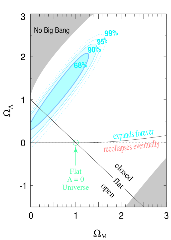
Figure 3.2: The best fit confidence regions in the ($\Omega_{m},\ \Omega_{\Lambda}$) plane obtained from the analysis of the Supernovae Cosmology Project (Perlmutter et al. 1999). The 68%, 90%, 95% and 99% confidence region are shown. The diagonal line corresponds to flat cosmology. Different cosmologies are also indicated.

The sample of the Supernova Cosmology Project is larger than HSST. Due to the large sample, the statistical uncertainty is small and the confidence region is narrow. It is also possible to estimate some systematic uncertainties in this case. In the flat case the value found is $\Omega_{m}=0.28\pm 0.085({\rm stat})\pm 0.05({\rm syst})$. The two-dimensional contour plot in the parameter space ($\Omega_{m},\ \Omega_{\Lambda}$) plane can be seen in fig. 3.2. We have used this data in our both analyses. None of the teams has considered the effect of galactic dust on the light curve. The effect of intergalactic dust on light curve has been described by Aguirre (1999). However, both supernova projects have concluded that the expansion of the Universe is accelerating. The coming SNAP satellite will be able to measure an enormous amount of distant supernovae every year. This can provide us essential information on the critical nature of the Universe.

3.3 Classical Double Radio Galaxies

Powerful extended classical double radio galaxies are used for constraining global cosmological parameters. It is much like the relation between supernovae and standard candles, comparing coordinate distance and powerful radio galaxies. At first Daly (1994, 1995) applied this method for constraining cosmological parameters and later adopted by others Guerra & Daly (1996, 1998), Guerra, Daly & Wan (2000).

It is observed that at a given redshift all radio sources have a similar size. This size may be estimated in two different ways: i) by the average size of the full population of powerful extended radio galaxies at that redshift; ii) by the product of average rate of growth of the source and the total time for the production of powerful jets. The two measures depend on the angular size distance to the sources, and the ratio of the two measures depend on the cosmological parameters $\Omega_{m},\Omega_{\Lambda}$, and a model parameter $\beta$. The rate of growth of the radio sources strongly depends on the redshift: it increases with redshift, but the average size of the full population decreases monotonically with redshift, for a redshift greater than 0.5.

In 1998, Daly, Guerra and Wan studied fourteen samples for constraining cosmological parameters. Guerra, Daly and Wan (2000) have identified 70 classical double radio galaxies with a redshift between zero and two. From there they have studied 20 of average size for constraining cosmological parameters. However, the likelihood contours in the ($\Omega_{m},\Omega_{\Lambda}$) plane available to us from this compilation correspond to 68% ($1\sigma$) and 90% ($1.64\sigma$) confidence, respectively. These confidence regions are quite large. This is therefore one of the weak constraints, thus affecting very little the total fit. For the $\chi^{2}$ analysis we introduced this constraint as a mathematical expression like Eq. (3.10) and Eq. (3.11), where the rotation angle is $\theta=70^{\circ}.4$ and the $w$ and $z$ errors are $\sigma_{w}=0.84,\sigma_{z}=0.33$. The same data have been introduced in the maximum likelihood analysis as a fifth order polynomial.

3.4 Gravitational Lensing

According to Einstein’s Theory of Relativity light rays are deflected due to the gravity of massive bodies. The deflection of light by massive bodies is known as Gravitational Lensing. From the gravitational lensing statistics, the matter distribution in the Universe can be studied. Distant objects (i.e. QSO’s) are usually used as a source of light. Galaxies or clusters of Galaxies are used as a lensing plane and on the Earth we are the observers. From this geometry one can establish a relation between an angular distance and the cosmological parameters at a given redshift.

Different techniques have been applied for constraining the cosmological parameters. Using the results from 5 optical quasar surveys, Cheng and Krauss (1998) have re-analyzed lensing statistics, and the best fit of $\Omega_{m}$ gives the maximum likelihood in the range between 0.25-0.55 in the flat Universe. Systematic uncertainties is dominant in this analysis, and the uncertainty comes mainly from the galaxy luminosity function and dark matter velocity dispersion. From the redshift survey of radio and optical data, Falco et al. (1998) have fitted the data independently and combined them. The confidence level is so wide that we can not even reach the lower limit of the contour.

Chiba & Yoshii (1999) have presented new calculations of gravitational lens statistics in view of the recently revised knowledge of the luminosity functions of elliptical (E) and lenticular (S0) galaxies and their internal dynamics. They applied their revised lens model to a sample of 867 unduplicated QSOs at $z>1$ taken from several optical lens surveys, as well as to 10 radio lenses. In sharp contrast to the previous models of lensing statistics that have supported a high-density universe with $\Omega_{m}=1$, they concluded that a flat universe with $\Omega_{m}=0.3^{+0.2}_{-0.1}$ casts the best case to explain the results of the observed lens surveys. Instead of using the above quoted $\Omega_{m}$ value, we use the 68% likelihood contour in the two-dimensional parameter space of Fig. 8 of Chiba & Yoshii (1999). We integrate out the characteristic velocity dispersion ($\sigma^{*}$), and we thus obtain the one-dimensional 68% confidence range $\Omega_{\Lambda}=0.70\pm 0.16$.

A preliminary result from the Cosmic Lens All-Sky Survey (CLASS) has been presented by Helbig (2000). Most probably this is the strongest constraint on the $(\Omega_{m},\ \Omega_{\Lambda})$ plane from lensing surveys. Although the maximum likelihood is wide, this is a strong constraint on $\Omega_{\Lambda}$. A large portion of the confidence level is in the region $\Omega_{\Lambda}$ $<$ 0 which may be considered unphysical. The upper bound of the contour may be interesting for $\Omega_{\Lambda}$ from this compilation. At this moment we get very little benefit from this result. However, we expect that in the near future it would be able to provide us with a strong constraint on the cosmological parameters. The likelihood contours in the ($\Omega_{m},\Omega_{\Lambda}$) plane available to us from this survey correspond to 68.3% ($1\sigma$), 90% ($1.64\sigma$), 95% ($1.96\sigma$), 99% ($2.58\sigma$) confidence, respectively.

3.5 Cluster Mass Function and Ly$\alpha$ Forest

The most common assumption is that the structure we observe today such as galaxies, clusters of galaxies and voids results from the growth of primordial density fluctuations by gravitational instability. These fluctuations are normally assumed to have originated from a Gaussian random process. The overdense regions will decelerate faster than the background Universe, because of their large gravitational field, resulting in an increase of their contrast relative to the background. If this deceleration is large enough, these regions will turn back and recollapse on themselves, resulting in the formation of positive density structures such as galaxies and clusters. The opposite phenomenon occurs in underdense regions. These regions decelerate more slowly than the background Universe, thus getting more underdense, and eventually become the cosmic voids we observe today.

Croft et al. (1998) have presented a theoretical model for recovering the linear power spectrum of mass fluctuations from high-redshift Quasi-stellar Object (QSO) Ly$\alpha$ spectra. They have tested the model by using 16 QSOs. For the precise measurement of $P(k)$ Croft et al. (1999) have combined 3 more samples at redshift 2.5 with their previous determination. Most recently, toward a more precise measurement of matter density, Croft et al. (2000) have used a wide number of samples (53 QSOs) of Ly$\alpha$ forest spectra in their analysis, discovered by the Keck telescope at redshifts between 2 and 4. Weinberg et al. (1999) estimated $\Omega_{m}$ by combining the cluster mass function constraint with the linear mass power spectrum determined from the Ly$\alpha$ data (Croft et al. 1998, 1999). For $\Omega_{\Lambda}=0$ they obtained $\Omega_{m}=0.46^{+0.12}_{-0.10}$ and for a flat universe they obtained $\Omega_{m}=0.34^{+0.13}_{-0.09}$. In the flat cosmology Croft et al. (2000) obtained $\Omega_{m}=0.50^{+0.13}_{-0.10}$.

3.6 Gas fraction in X-ray clusters

Clusters emit X-rays which indicates that the clusters consist of a large amount of hot gas. From the measurement of the gas fraction in X-ray clusters one can reach the Universal matter density $\Omega_{m}$. It is observed that at a certain radius, the clusters are in hydrostatic equilibrium. This radius is known as the virial radius. A common definition of the virial radius is $R_{500}$; outside this radius the density drops below 500 in units of the critical density (Navarro, Frenk & White 1995). All matter outside the virial surface are infalling with the cosmic mix of components. Then the baryonic mass fraction measured at the virial radius must be unbiased. Thus, by measuring the gas fraction near the virial radius, one expects to obtain fairly unbiased information on the ratio of $\Omega_{m}$ to the cosmic baryonic density parameter $\Omega_{b}$. This type of analysis has been done before (Evrard 1997) using the best known value of $\Omega_{b}$ to derive a value of $\Omega_{m}$. In Chapter 5, we do the opposite: we use our best estimation of $\Omega_{m}$ to determine some poorly known parameters.

For this purpose Evrard (1997) has used a very large sample of clusters: the ROSAT compilation of David, Jones & Forman (1995) and the Einstein compilation of White & Fabian (1995). He has obtained a realistic value of

$${\Omega_{m}\over\Omega_{b}}h^{-4/3}\approx(11.8\pm 0.7)\ .$$ (3.12)

This value includes a galaxy mass estimate of 20% of gas mass, and a baryon diminution $\Upsilon(500)=0.85$ at $R_{500}$ (a detail definition of $\Upsilon$ can be found in Section 5.4). To get a precise information on the density parameter $\Omega_{m}$, we need the precise values of $\Omega_{b}$ and $h$. The problem lies in the contradiction in baryonic density between the Big Bang Nucleosynthesis (BBN) and the Cosmic Microwave Background (CMB) observations by the recent balloon experiments BOOMERANG (2000) and MAXIMA-1 (2000). However, taking $\Omega_{b}=0.020\pm 0.001h^{-2}$ (68% CL) from the low primordial deuterium abundance (Burles et al. 2001), and $h=0.73\pm 0.07$ (68% CL) Gibson & Brook (2001) who have re-analyzed Calan-Tololo and the Center for Astrophysics (CfA) SNe Ia datasets, one obtains $\Omega_{m}=0.29\pm 0.11$.

3.7 Power Spectrum of Galaxy Fluctuations

Matter in every direction appears to be distributed in high-density peaks separated by voids. The average separation distance is $\sim 130h^{-1}$Mpc, which translates into a peak in the power spectrum of mass fluctuations. This provides a co-moving scale for measuring cosmological curvatures. Broadhurst & Jaffe (1999) used a set of Lyman galaxies at $z\sim 3$ finding a constraint in the form $\Omega_{m}=0.20\pm 0.10+0.34\Omega_{\Lambda}$. Roukema & Mamon (1999) have carried out a similar analysis of quasars, finding $\Omega_{m}=0.24\pm 0.15+(0.10\pm 0.08)\Omega_{\Lambda}$.

The distribution of galaxies is considered to be Gaussian. For the peaks measurements, small angle geometry with the normal could provide precise information of the co-moving scale. The density parameters $\Omega_{m}$, $\Omega_{\Lambda}$ measured from these observations lie between the locii of supernovae and cosmic microwave background, that is, $(3\Omega_{m}-\Omega_{\Lambda})$.

3.8 Galaxy Peculiar Velocities

The large-scale peculiar velocities of galaxies correspond via gravity to mass density fluctuations about the mean, and depend also on the mean density itself. Two catalogs of galaxies have been analyzed for these velocities in order to provide information on $\Omega_{m}$: the Mark III catalog (Willick et al. 1997) of about 3000 galaxies within a distance of $\sim 70h^{-1}$ Mpc, and the SFI catalog (Borgani et al. 1999) of about 1300 spiral galaxies in a similar volume. Combining the results in these catalogs, Zehavi & Dekel (1999) quote the constraint

$$\Omega_{m}\ h_{65}^{1.3}\ n^{2}\simeq 0.58\pm 0.12\ ,$$ (3.13)

in the case of flat cosmology, where the error corresponds to a 90% confidence level. Taking the index $n$ of the mass-density fluctuation power spectrum to be $n=1.0\pm 0.1$ (Bond & Jaffe 1998), one obtains the constraint $\Omega_{m}=0.55\pm 0.14$, where the error corresponds to a 68% confidence level.

3.9 X-ray Cluster Evolution

The Clusters of Galaxies are the largest known gravitationally bound and the most massive objects in the Universe. Massive clusters are more luminous and they emit X-rays. It is observed that the evolution of the number density of rich cluster galaxies breaks the degeneracy between the Universal mass density and the normalization of the power spectrum $\sigma_{8}$. This evolution is strong with high-mass and low-$\sigma_{8}$ models. The number density of clusters decreases by a factor of $10^{3}$ from $z=0$ to $z=0.5$. The same clusters show mild evolution in low-mass and high-$\sigma_{8}$ models, the decrease is by a factor of 10. Bahcall et al. (1997, 1998), Eke et al. (1998), Viana & Liddle (1999), Moscardini et al. (2000) have used this degeneracy as a powerful tool for the constraint on cosmological parameters. Note that this evolution is strongly model dependent. In the next Chapter we have analyzed the recent Advanced Satellite for Cosmology and Astrophysics (ASCA) data for the study of baryonic dark matter.

There are still a few more constraints that have been used in the $\chi^{2}$ analysis. For critical evaluation of the density parameters $\Omega_{m}$ and $\Omega_{\Lambda}$ we have done another combined study in the Paper (IV). The rest of the constraints have been discussed in Paper (IV), and they will be discussed also in the next Chapter. The data used in the $\chi^{2}$ method are summarized in tables 3.1 and 3.2.

Sources	$\Omega_{m}$	$\Omega_{\Lambda}$	$\Omega_{0}=\Omega_{m}+\Omega_{\Lambda}$	References
High-Z SN Ia	$0.20\pm{0.22}$	$0.65\pm{0.28}$	$0.85\pm{0.35}$	[100]
SCP	$0.28_{-0.13}^{+0.19}$	$0.73_{-0.22}^{+0.19}$	$1.01_{-0.25}^{+0.26}$	[94]
Double Radio Galaxies	$0.09_{-0.09}^{+0.29}$	correlated	–	[49]
Various CMBR data	correlated	correlated	–	[70]
BOOMERANG CMBR	–	–	$1.03_{-0.06}^{+0.07}$	[29]
MAXIMA-1 CMBR	–	–	$0.90\pm{0.08}$	[6]

Table 3.1: Two-dimensional data in the $\chi^{2}$ analysis. All errors are given at 1$\sigma$ confidence level.

Sources	$\Omega_{m}^{flat}$	$\Omega_{\Lambda}^{flat}$	References
Galaxy Power Spectrum	$0.40\pm{0.10}$	$1-\Omega_{m}$	[13]
Gravitational Lensing	$1-\Omega_{\Lambda}$	$0.70\pm{0.16}$	[22]
Gravitational Lensing	$1-\Omega_{\Lambda}$	$0.64\pm{0.15}$	[57]
Ly$\alpha$ Forest	$0.34_{-0.09}^{+0.13}$	$1-\Omega_{m}$	[124]
Temperature-Redshift	$0.27\pm{0.10}$	$1-\Omega_{m}$	[31]
Galaxy Peculiar Velocities	$0.55\pm{0.14}$	$1-\Omega_{m}$	[129]
X-ray Clusters	$0.36\pm{0.09}$	$1-\Omega_{m}$	[36]
Large Scale Structure	$0.30\pm{0.15}$	$1-\Omega_{m}$	[106]
Cluster Evolution	$0.45\pm{0.20}$	$1-\Omega_{m}$	[33]

Table 3.2: One-dimensional (flat space) data in the $\chi^{2}$ analysis. Errors are given at 1$\sigma$ confidence level.

3.10 Data Analysis: $\chi^{2}$ Method

The $\chi^{2}$ statistics is one of the strongest mathematical tools that has been successfully used for experimental and observational data analyses. It is used to investigate whether the distributions differ from one another, and of course to find the best estimation from a set of data. A confidence level is also determined from the combined distribution. The $\chi^{2}$ statistics is calculated as

$$\chi^{2}=\sum_{i}{(O_{i}-E_{i})^{2}\over e_{i}},$$ (3.14)

where $O_{i}^{{}^{\prime}s}$ are the observed and $E_{i}^{{}^{\prime}s}$ are the expected values.

Using two free parameters $\Omega_{m}$, $\Omega_{\Lambda}$, we have performed a $\chi^{2}$ fit to the constraints summarized in the tables 3.1 and 3.2, assuming that all reported observational errors as well as systematic errors are Gaussian. For this analysis we use MINUIT standard program for function minimization and error calculation (James & Roos), which is available from the CERN Program Library and is documented there as entry D506. We fit the data in two different cases: one-dimensional and two-dimensional. The two-dimensional best fit value is found to be $\Omega_{m}=0.33\pm 0.07$, $\Omega_{\Lambda}=0.66\pm 0.12$, thus $\Omega_{m}+\Omega_{\Lambda}=0.99\pm 0.14$, where the errors are estimated for 1$\sigma$ (CL). In the exact flatness case we have found $\Omega_{m}=0.33\pm 0.04$, $\Omega_{\Lambda}=0.67\pm 0.04$. The interesting thing is that there is no remarkable change in the parameters but the errors decrease because the dimensional space is one. To find the absolute 1$\sigma$ and 2$\sigma$ confidence regions in the $\Omega_{m}$, $\Omega_{\Lambda}$-plane we add $\Delta\chi^{2}$ = 2.3 and 6.2 up from the minimum, respectively. Our $\chi^{2}$ fit is extremely good. That can be seen from the degrees of freedom. In the two-dimensional fit and for ten constraints, $\chi^{2}$ is 4.42, where the degrees of freedom is 8, and in the one-dimensional case $\chi^{2}$ is 4.43 where the degrees of freedom is 9. In the two-dimensional case, a fit is good when $\chi^{2}$ is about N - 2, where N is the total number of constraints. Therefore the goodness-of-fit here is extremely high.

It is obvious that the greater the discrepancy between observed and adjusted values, the greater will be the value of $\chi^{2}$. To check this argument we have measured the individual $\chi^{2}$ for each observational data set. In our ten constraint analysis the maximum $\chi^{2}$ comes from the CMBR data, but it is still very small: slightly less than one.

We have also fitted the data without the SN Ia constraints. We found very little change. The result is then $\Omega_{m}=0.34\pm 0.07$, $\Omega_{\Lambda}=0.64\pm 0.09$, thus $\Omega_{m}+\Omega_{\Lambda}=0.98\pm 0.11$. The reason is that there are strong constraints, for instance, gravitational lensing on $\Omega_{\Lambda}$ and gas fraction in X-ray clusters on the $\Omega_{m}$, and they constrain the result similarly. We did not measure any systematic error from this fit. If we carefully observe, we do not need to estimate the systematic errors. The data we have used here pull in randomly different directions. It means that the CMB constraint is laying along the flat line, supernova constraints are orthogonal to the CMB constraint. Again the gas fraction in X-ray cluster constraints is perpendicular to the gravitational lensing, and the distribution of others is quite random. Thus, the total effect might be a mutual cancellation. So we can say that the systematic errors are already included. In such situation there is no reason to reconsider the effects of systematic errors.

There can be more arguments against the systematic errors. Why does one neglects them in this analysis? In fact, most of the constraints have come from fits of higher dimensions. We do not have any information whether the parameters have been properly rescaled or not for the lower dimensionality. Overall, we think that our errors have already been generous, and there is no motivation to add further systematic errors arbitrarily.

Later, we combined a few more constraints in our $\chi^{2}$ fit Paper (III), where the total number of constraints were sixteen. From the overall analysis, it was shown that the flatness of the Universe is robust.

However, it is observed that a large number of data are not Gaussian, the best value is also being unknown in some cases. In such a situation, we loose information about the input data. Taking these points into consideration, a critical analysis has been done in the Paper IV. The limitations and advantages of $\chi^{2}$ and maximum likelihood method have been described in Paper IV. Some of the constraints that will be used in the maximum likelihood analysis have already been discussed in this Chapter.

Figure 3.1: Top: CMB power spectra from BOOMERANG, MAXIMA-1 and COBE-DMR. Bottom: Beam calibration uncertainties are used to adjust the peaks (Jaffe et al 2000.)

Chapter 4 Observational Data Analysis

Different groups have combined data from different observations, e.g. Lineweaver (1999) combined the supernovae data with Cosmic Microwave Background (CMB) data, X-ray cluster data, cluster evolution data and double radio sources. Le Dour et al. (2000) analysed only Cosmic Microwave Background data, whereas Tegmark et al. (2000a) combined them with Infrared Astronomical Satellite (IRAS) Large Scale Structure (LSS) data. Tegmark & Zaldarriaga (2000b, 2000c) and Hu et al. (2000) combined BOOMERANG and MAXIMA data, Melchiorri et al. (2000) combined BOOMERANG and Cosmic Background Explorer (COBE) data. Bridle et al. (2000) combined the Cosmic Microwave Background data with galaxy peculiar velocities and the supernovae data. The balloon data have been combined with LSS and supernovae data by Jaffe et al. (2000) and by Bond et al. (2000), and with a different set of LSS data by Novosyadlyj et al. (2000a) and Durrer & Novosyadlyj (2000). We have done a critical combined study using Maximum Likelihood method. The main interest herein is the following: i) taking care of statistics; ii) a combined two-dimensional output contour and the best value using individual two-dimensional contours as input; iii) agreement and disagreement of data with each other. In this analysis we have used supernovae data (Riess et al. 1998, Perlmutter et al. 1999), CMB data (Tegmark 1999, de Bernardis et. al. 2000, Balbi et al. 2000, Hanany et al. 2000), LSS data (Novosyadlyj et al. 2000b) and Double Radio Galaxies data (Guerra el al. 2000).

4.1 Maximum Likelihood Method

This is another mathematical tool that has been used for the data analysis. From the statistical and theoretical point of view, the best method for the data analysis with a high resolution is so far the maximum likelihood method. The likelihood function for a set of data is the joint probability density function (pdf) of the data, given some parametric model. The values of the parameters maximize the sample likelihood. In principle, we can obtain the $\chi^{2}$ from the maximum likelihood. For a normally distributed variable $\chi^{2}$ is the negative logarithm of the maximum likelihood. So, we can say that maximum likelihood is optimal, and $\chi^{2}$ is a special case of maximum likelihood. The advantage of the maximum likelihood method is that we can use all kinds of data as an input with more precision, details of which may be found in Paper (IV).

We have represented the confidence contours of the data by fifth order polynomials of the form

$$P(\Omega_{m}\Omega_{\Lambda})=\Omega_{m}^{m}\Omega_{\Lambda}^{n},(m+n)\leq 5.$$ (4.1)

There are 20 terms in the polynomials. Therefore we read off 20 points from the $1\sigma,\ 1.64\sigma,\ 2\sigma,\ 3\sigma$ contours and the best value, if available. Here we get a 20 x 20 matrix. We invert the matrix once and multiply with the data points that are taken from the contours. The equation is then ready to describe the nature of data. Since we already know the approximate location of the globally favored region from all previous studies, we can take care of that our polynomial approximation is good over that region. This fit region is defined by $0.15\leq\Omega_{m}\leq 0.50$ and $0.40\leq\Omega_{\Lambda}\leq 0.88$, but the sample points are taken also from outside this region in order to obtain a well-behaved polynomial inside the region. Far away from it, the polynomial approximation of course breaks down completely.

We have taken special care of each data set. We have checked that the polynomial is non-negative in the fit region. We have also examined the location of the 0.33$\sigma$ contour, in order to verify that the region is reasonably centrally located. Note that one can use higher order polynomials for better accuracy but it would be very difficult to control the polynomial; even in the fifth order polynomial we need some constraints to adjust the data points up to the sixth decimal.

In the previous Chapter, we have described the two well known analyses from the supernovae observations and their results. Since we know that the supernovae observations constrain essentially only the $\Omega_{\Lambda}-\Omega_{m}$ parameter combination, let us compare their results along the $\Omega_{\Lambda}-\Omega_{m}$ direction, where they have used the same method. Along the flat line the result is then $\Omega_{\Lambda}-\Omega_{m}=0.44\pm 0.10$ for Supernovae Cosmology Project (SCP) (Perlmutter et al. 1999), and $\Omega_{\Lambda}-\Omega_{m}=0.36\pm 0.10$ for the High Redshift Supernovae Search Team (HSST) (Riess et al. 1998). A 5% systematic uncertainty have been included in the SCP result but we do not have any information about the systematic uncertainty for the HSST case. However, the two observations then agree within their statistical errors.

Now we shall see the combined results of these two observations. In Fig. 4.1 we show the confidence contours of the log-likelihood sum of the two observations in our polynomial approximation, drawn only in the above mentioned ranges of $\Omega_{m}$ and $\Omega_{\Lambda}$. Along the flat line these experiments determine $\Omega_{\Lambda}-\Omega_{m}=0.45\pm 0.13$. The SCP result is stronger than that of HSST. Therefore, the best fit is moved toward the SCP but the combined contour is naturally wider.

Figure 4.1: Confidence contours of the log-likelihood sum of two SN Ia observations (HSST and SCP). The inner and outer curves corresponds to 1$\sigma$ and 2$\sigma$ in the ($\Omega_{m},\ \Omega_{\Lambda}$)-plane, respectively. The significance of the square is described in the text. The diagonal line corresponds to a flat cosmology.

Constraints on cosmological parameters from earlier Cosmic Microwave Background Radiation (CMB) and Double Radio Galaxies has also been described in the previous Chapter. By CMB we mean only the observations summarized by Lineweaver (1998) and Tegmark (1999), not including BOOMERANG and MAXIMA-1 which we treat separately. CMB puts a strong constraint along the direction $\Omega_{0}=\Omega_{m}+\Omega_{\Lambda}=1$. The combination of supernovae with CMB is also well known. It can be interesting to combine Double Radio Galaxies with supernovae and CMB. In Fig. 4.2 we show the confidence contours of the log-likelihood sum of two supernovae (HSST and SCP), CMB and Double Radio Galaxies in our polynomial approximation, drawn only in the ranges of $\Omega_{m}$ and $\Omega_{\Lambda}$ that we sample. The Double Radio Galaxies is so far a weak constraint on $\Omega_{m}$ and $\Omega_{\Lambda}$. Thus the confidence region is mostly dominated by supernovae and CMB.

Figure 4.2: The confidence contours of the log-likelihood sum of two SN Ia (HSST and SCP), CMB and Double Radio Galaxies. The inner and outer curves correspond to 1$\sigma$ and 2$\sigma$ in the ($\Omega_{m},\ \Omega_{\Lambda}$)-plane, respectively. The significance of the square is described in the text. The diagonal line corresponds to a flat cosmology.

4.2 Balloon Experiments

The recent two balloon experiments BOOMERANG (de Bernardis et al. 2000) and MAXIMA-1 (Balbi et al. 2000, Hanany et al. 2000) have given us a most exciting information in observational cosmology. The two experiments are held in two different parts of the world. BOOMERANG is held in Antarctica and the MAXIMA-1 in California. There is a big exposed time difference between two observations. BOOMERANG was flown 11 days for the data collection whereas MAXIMA-1 was flown only for 2 hours. According to their best estimation, BOOMERANG has hinted that the Universe is might even be closed. However, MAXIMA-1 tells us that the Universe is open. On one hand we can not escape from the statistical fluctuations, and on the other hand there could be some important corrections in the theory. Let us now turn to the theory. The widely used formula is that the first peak corresponds to a flat cosmology, and it was derived by Kamionkowski et al. (1994) for the case $\Omega_{\Lambda}=0$ as

$$\ell_{1}\simeq 200{\Omega_{0}}^{-0.5}$$ (4.2)

For the case $\Omega_{m}=0.3$ and $\Omega_{0}$ near 1 Weinberg (2000) has derived the relation

$$\ell_{1}\simeq 200{\Omega_{0}}^{-1.58}.$$ (4.3)

Near $\Omega_{0}=1$ the relation (4.2) and (4.3) are of course very similar. Let us now turn to their results. BOOMERANG observes (de Bernardis et al. 2000) that the position of the first multipole peak occurs at $\ell_{1}=197\pm 6$ which corresponds to

$$\Omega_{0}=(200/\ell_{1})^{2}=1.01\pm 0.02\ .$$ (4.4)

This value is very weakly dependent on a large number of parameters which mostly get determined by the shape of the multipole spectrum above the region of the first peak (Lange et al. 2000). Actually BOOMERANG and MAXIMA-1 fit their multiparameter data by the program CMBfast, so they do not explicitly use either (4.2) or (4.3). For the BOOMERANG results, there are no precise confidence levels published, only a coarsely pixelized likelihood surface of 95% confidence. Other confidence contours such as 68% CL, 90% CL are not reported. In consequence we do not have sufficient information to use our polynomial fit to the data. Of course the maximum likelihood method can compute these confidence contours by using the 95% CL information above, but this is not reliable at all. Therefore, we did not include the BOOMERANG data as an independent constraint, but it has been included together with the Large Scale Structure constraint (Novosyadlyj et al. 2000b).

Now we turn to MAXIMA-1. From the statistical point of view this is less precise than that of BOOMERANG. They find the first acoustic peak at $\ell_{1}\simeq 210$. Therefore, we are not surprised about the report of Balbi et al. (2000) $\Omega_{0}=0.90\pm 0.15$, where the error corresponds to a 95% confidence level. If we convert this to a 68% error, then $\Omega_{0}=0.90\pm 0.08$. The likelihood contours in the $\Omega_{m},\Omega_{\Lambda}$ plane from MAXIMA-1 (Balbi et al. 2000) are available to us 68% $(1\sigma)$, 95% $(1.96\sigma)$ and 99% $(2.58\sigma)$ confidence levels respectively.

There is a contradiction in the acoustic peaks between the two observations. There is no clear information from where the difference comes. Nevertheless, both teams are analysing additional data which may reduce the conflict of the region of power spectrum where further peaks are expected. In the meantime, to adjust the peaks between these two experiments, a clever technique has been applied by Jaffe et al. (2000). Both teams BOOMERANG and MAXIMA-1 have a remarkable calibration uncertainty in their method. Jaffe et al. (2000) have used this uncertainty for the adjustment of the peaks. The new acoustic peak is then between BOOMERANG and MAXIMA-1. MAXIMA-1 $\downarrow$ and BOOMERANG $\uparrow$ Fig. 3.1.

Let us see our confidence region including balloon data. In Fig. 4.3 we show the confidence contours of the log-likelihood sum of the SNe Ia, CMB, Double Radio Galaxies and MAXIMA-1. We have not yet included BOOMERANG data in this fit. It will be included with LSS in the total fit. We have plotted our polynomial approximation only in the chosen window of $\Omega_{m}$ and $\Omega_{\Lambda}$.

Figure 4.3: Confidence contours of the log-likelihood sum of two SN Ia (HSST and SCP), CMBR, Double Radio Galaxies and MAXIMA. The inner and outer curves correspond to 1$\sigma$ and 2$\sigma$ in the ($\Omega_{m},\ \Omega_{\Lambda}$)-plane, respectively. The significance of the square is described in the text. The diagonal line corresponds to a flat cosmology.

4.3 Large Scale Structure

Today’s great challenge of science is to understand the structure of our Universe. One widely used theory on observational cosmology concerns structure formation yielding Large Scale Structures (LSS), and it was originated from the theory of Big Bang. The form of the power spectrum strongly depends on the cosmological parameters. From the observation of the power spectrum of density fluctuations one can apply a constraint on $\Omega_{m}$, $\Omega_{\Lambda}$. In a series of Papers Novosyadlyj et al. (1999, 2000a, 2000b, 2000c), Durrer and Novosyadlyj (2000) have analysed up to eight parameters in the $\chi^{2}$ fit to obtain the cosmological parameters. They have used the constraint on the amplitudes of power spectrum fluctuations from different sources on a wide scale. They have combined the power spectrum of density fluctuations of Abell-ACO clusters of Retzlaff et al. (1998) with optical determinations of the mass function of nearby galaxy clusters by Girardi et al. (1998), with evolution of the galaxy cluster X-ray temperature distribution function by Viana & Liddle (1999a), Bahcall & Fan (1998), with a study of bulk flows of galaxies by Kolatt & Dekel (1997), and with Ly-$\alpha$ absorption lines in quasar by Gnedin (1998), Croft et al (1998). They apply a constraint on baryon density from big bang nucleosynthesis (BBN) by Burles et al. (1999), and the value of the Hubble constant $h=0.65\pm 0.10$. The Hubble value is low but reasonable within errors. The position of the first acoustic peak from the BOOMERANG observations, $\ell_{1}=197\pm 6$, has also been included in their analysis.

There are seven continuous free parameters in this fit. They have fitted the parameters for a fixed neutrino number density ($N_{\nu}$ = 1, 2, and 3) in a mixed dark matter model with a cosmological constant ($\Lambda$MDM). The $\chi^{2}$ is minimal for one species of massive neutrinos, and the values of mass density and vacuum energy density are then $\Omega_{m}=0.37_{-0.15}^{+0.25}$, $\Omega_{\Lambda}=0.69_{-0.20}^{+0.15}$. The likelihood contours in the $\Omega_{m},\Omega_{\Lambda}$ plane from LSS (Novosyadlyj et al. 2000c) are available to us 68.3% $(1\sigma)$, 95.4% $(2\sigma)$ and 99.73% $(3\sigma)$ confidence level, respectively.

In Fig. 4.4 we show the confidence contours of the log-likelihood sum of CMB, MAXIMA-1, LSS and Double Radio Galaxies. We have plotted our polynomial approximation only in the ranges of $\Omega_{m}$ and $\Omega_{\Lambda}$ that we sampled. As can be clearly seen, the likelihood function contains information mainly on $\Omega_{0}$, but it also gives a rather conspicuous upper limit on the orthogonal combination $\Omega_{\Lambda}-\Omega_{m}$. The narrowness in this fit mainly comes from the CMB and MAXIMA-1.

Figure 4.4: The confidence contours of the log-likelihood sum of CMBR, MAXIMA-1, LSS and Double Radio Galaxies. The inner and outer curves correspond to 1$\sigma$ and 2$\sigma$ in the ($\Omega_{m},\ \Omega_{\Lambda}$)-plane, respectively. The significance of the square is described in the text. The diagonal line corresponds to a flat cosmology.

4.4 Fitting and Errors

Adding up our polynomial approximations to the confidence contours of all the data fitted in this section, results in Fig. 4.5, where we show the location of the minimum, the $1\sigma$ and $2\sigma$ contours. From this Figure one can read off the following results:

$$\Omega_{m}=0.31^{+0.12}_{-0.09}$$ (4.5)

$$\Omega_{\Lambda}=0.68\pm 0.12,$$ (4.6)

or alternatively

$$\Omega_{0}=0.99\pm 0.04$$ (4.7)

$$\Omega_{\Lambda}-\Omega_{m}=0.37^{+0.20}_{-0.23}.$$ (4.8)

Figure 4.5: All the constraints described in this Chapter combined. The ’+’ marks the best fit: ($\Omega_{m},\ \Omega_{\Lambda}$) = (0.31,0.68). The inner and outer curves correspond to 1$\sigma$ and 2$\sigma$ in the ($\Omega_{m},\ \Omega_{\Lambda}$)-plane, respectively. The diagonal line corresponds to a flat cosmology.

Of these results, only the determination of $\Omega_{0}$ is quite precise and worth detailed attention. We can conclude from it that a flat universe with $\Omega_{0}=1$ is very likely.

The error of $\pm 0.04$ is mainly statistical, although it does contain systematic errors due to mildly discordant experiments, as discussed in the previous section. To this we have to add a total systematic error which we evaluate as follows.

Before discussing the systematic errors let us see the results taking into account the new result of lensing statistics Helbig (2000). As we know that there is a strong disagreement between lensing and supernovae data, it could be interesting just to see the combined results. We combine lensing data Helbig (2000) with fig. 4.5, the total results is then $\Omega_{m}=0.34_{-0.03}^{+0.11}$, $\Omega_{\Lambda}=0.63_{-0.10}^{+0.04}$ or alternatively $\Omega_{0}=0.97_{-0.04}^{+0.05}$ $\Omega_{\Lambda}-\Omega_{m}=0.29_{-0.18}^{+0.05}$. The best value is excluded by the supernovae data at 1$\sigma\ {\rm CL}$, and it is excluded by lensing data at 97% ${\rm CL}$. For this strong contradiction the nice shape of the contour plot is destroyed; that may be seen in the Paper IV fig. 4.

Perlmutter et al. (1998, 1999) have quoted a total systematic error for $\Omega_{m}$ and $\Omega_{\Lambda}$ along the flat line of $\pm 0.05$. We consider that the same error applies to the SN Ia data of Riess et al. (1998), although they could not evaluate it from their limited sample of SNe Ia. Displacing both the SN Ia contours by $\pm 0.05$ along the flat line, we obtain a very small systematic error in the $\Omega_{0}$ direction

$$\Delta_{1}\Omega_{0}=^{+0.012}_{-0.006}.$$ (4.9)

There are also two kinds of systematic errors inherent in our method of analysis. Firstly, we are reading off the coordinates of the confidence contours of the different experiments with some finite precision. We estimate this to be

$$\Delta_{2}\Omega_{0}=0.027.$$ (4.10)

Secondly, since we only use 20 points to fit the confidence contours of each experiment, there is an arbitrariness in their choice; all we require is that the confidence contours should be well fitted by whichever polynomial. This polynomial arbitrariness results in a systematic error estimated to be

$$\Delta_{3}\Omega_{0}=0.01.$$ (4.11)

The quadratic sum of the errors in Eqs. (4.9), (4.10), (4.11) is then

$$\Delta_{tot}\Omega_{0}=0.03.$$ (4.12)

Thus our final result for $\Omega_{0}$ is

$$\Omega_{0}=0.99\pm 0.04\pm 0.03,$$ (4.13)

where the first error is statistical and the second error is systematical. Thus our total error is $\pm 0.05$.

Let us now turn to the case of exact flatness, $\Omega_{m}=1-\Omega_{\Lambda}$. Along the flat line the SN Ia systematic error is somewhat larger than in the case of Eq. (4.9),

$$\Delta_{1}\Omega_{0}^{flat}=\pm 0.025.$$ (4.14)

Our result is then

$$\Omega_{m}^{flat}=0.31\pm 0.04\pm 0.04,$$ (4.15)

where the first error is statistical and the second error is systematical. Thus our total error is $\pm 0.055$.

The overall constraints on cosmological parameters in year 2001 are summarized in table 4.1

Parameters	values	References
$\Omega_{m}$	$0.31\pm{0.06}$	Harun-or-Rashid & Roos 2001
$\Omega_{\Lambda}$	$0.68\pm{0.07}$	Harun-or-Rashid & Roos 2001
$\Omega_{0}$	$0.99\pm{0.04}$	Harun-or-Rashid & Roos 2001
$t_{0}$	$13.5\pm{1.3}$	Roos & Harun-or-Rashid 2001
$H_{0}$	$73\pm{7}$	Gibson & Brook 2001
$\Omega_{b}h^{2}$	$0.020\pm 0.001$	Burles et al. 2001 (BBN)
$\Omega_{b}h^{2}$	$0.022_{-0.003}^{+0.004}$	de Bernardis et al. 2001 (CMB)
$\alpha$	-1 $<$  but $<$ - ${1\over 3}$	Perlmutter et al. 1999 (SNe Ia)
$\alpha$	-1 $\leq$  but $<$ - ${1\over 2}$	Bludman & Roos 2001 (Quintessence)

Table 4.1: Constraints on cosmological parameters. Errors are given at 1$\sigma$ confidence level. The Hubble constant $H_{0}$ in units of $\rm{km\ s^{-1}Mpc^{-1}}$ and $t_{0}$ is in Gyr.

Chapter 5 Search for Baryonic Dark Matter in Clusters

5.1 What is Dark Matter?

Observations tell that more than 90% matter in the Universe is dark, but it is mostly obscure to the physicist and astronomer. In general, any form of matter which exists in the Universe in a non-luminous form is called dark matter. Two types of dark matter exist, namely baryonic dark matter and non-baryonic dark matter. The main baryonic dark matter candidates are Massive Compact Halo Objects (MACHOs), white, red and brown dwarfs, planetary objects, neutron stars, black holes, dust clouds. The MACHO collaboration (Alcock et al. 1997, 2000) has surveyed the halos in the Large Magellanic Cloud (LMC) and the Small Magellanic Cloud (SMC) at different scales. Searching for microlensing events toward LMC Alcock et al. (2000) reported that the most likely MACHOs mass is between $0.15M_{\odot}$ and $0.9M_{\odot}$. Among known astrophysical objects white dwarfs is in this mass range, so they are good candidates for MACHOs. Most recently, a large number of dead stars have been detected at the edge of our galaxy, the Milky Way (Oppenheimer et al. 2001). Extensions of the Standard Model of Particle Physics provide non-baryonic candidates to dark matter. From the cosmological point of view two main categories of non-baryonic candidates have been proposed: Cold Dark Matter (CDM) and Hot Dark Matter (HDM) according to whether they were slow or fast moving at the time of the galaxy formation. The typical HDM candidates are neutrinos of a few eV, whereas in the CDM sector, typical candidates are heavy Dirac or Majorana neutrinos in the GeV-TeV mass range or Weakly Interacting Massive Particles (WIMPs) with unknown properties. Supersymmetric theories offer a number of candidates, such as neutralinos and axions.

A good object for the study of baryonic dark matter in the Universe is a cluster of galaxies. The size of the clusters are big and the edges are not well defined. At large distance from the cluster center their properties approach average universal properties. For this analysis Advanced Satellite for Cosmology and Astrophysics (ASCA) data will be used from the six X-ray clusters A401, A496, A2029, A2199, A2256, A3571. A precise value of $\Omega_{m}$ can be used in different contexts. Our new result of $\Omega_{m}$ from the Chapters III and IV will be used for the analysis of baryonic dark matter in these clusters. Note that this data set has also been analyzed by Nevalainen et al. (1999, 2000a, 2000b) for constraining cosmological parameters. The measurement of gas fraction in these clusters resembles their analysis.

5.2 Clusters of Galaxies

Clusters are composed of baryonic and non-baryonic matter. The baryonic matter takes the forms of hot gas emitting X-rays, stellar mass observed in visual light, and perhaps invisible baryonic dark matter of unknown composition. Let us denote the respective fractions as $f_{gas},\ f_{gal}$, $f_{bdm}$. It has been observed in a large number of clusters that $f_{gas}$ is an increasing function of radius (e.g. White & Fabian 1995; Markevitch et al. 1997, 1999; Ettori & Fabian 1998; Nevalainen et al. 1999, 2000b), approaching the universal ratio at a large radius, as deduced from cluster formation simulations (e.g. White et al. 1993, Frenk et al. 1999, Tittley & Couchman 2000). Denoting the universal baryonic density parameter as $\Omega_{b}$ and the universal total mass density parameter as $\Omega_{m}$, one can write

$$f_{gas}(r)+f_{gal}(r)+f_{bdm}(r)=\Upsilon(r){\Omega_{b}\over\Omega_{m}}\ ,$$ (5.1)

where $\Upsilon(r)$ describes the possible local enhancement or diminution of baryon matter density in a cluster, compared to the universal baryon density. One can make different conclusions from the Eq. 5.1. Let us turn to known and unknown quantities in Eq. (5.1). The value of $\Omega_{m}$ is precisely known (Paper IV) and $\Upsilon$ is known with error and there is a strong constraint on it from simulations by Frenk et al. (1999). If we trust observational data, $f_{gas}(r)$ is known from fig. 5.1, the value of baryonic density $\Omega_{b}$ is also known but contradictory between BBN and CMB (as has been discussed in the previous Chapters). The unknown or poorly known quantity in the above expression is $f_{bdm}$. Until the contradiction is resolved, the baryonic density can be used from BBN and CMB independently.

It has been known before that the gas fractions in clusters of galaxies are too high for Eq. (5.1) to be satisfied with $\Omega_{m}=1$ (e.g. White et al. 1993; David et al. 1995; White & Fabian 1995; Ettori & Fabian 1998; Mohr et al. 1999). The qualitative conclusion given by the lower accepted limit for $\Omega_{m}$ is that a large fraction of baryonic matter other than gas is ruled out. Using up-to-date data on $f_{gas}$, $\Omega_{b}$, $\Omega_{m}$, $\Upsilon$ and $H_{0}$ one can set a quantitative limit to the sum of $f_{gal}$ and $f_{bdm}$ using Eq. (5.1).

5.3 Gas Fraction

Usually the total masses and gas fractions have been determined using the hydrostatic equilibrium condition with an isothermal assumption for the cluster gas. Here we have abandoned the isothermality assumption and instead derived the gas mass fraction $f_{gas}(r)$ from a sample of six clusters, whose total mass profiles have been determined using the gas temperature profiles observed with ASCA. For this derivation I am indebted to Jukka Nevalainen. This is an important improvement upon the earlier work, because the accuracy of the total mass within a given radius is approximately proportional to the accuracy of the gas temperature at that radius. The gas mass profiles have been obtained from the ROSAT imaging data (see Nevalainen et al. (2000a) and the references therein for the original hydrostatic mass analyses of the individual clusters in the sample).

We averaged the individual $f_{gas}(r)$ profiles without weighing them with their errors because the errors are not comparable due to different modeling of the temperature data in different cases. As the $1\sigma$ error of the average we took the standard deviation of their distribution (the square root of the unbiased variance of the data set). As a radial parameter we used the overdensity, or the mean total mass density within a given radius in units of the critical density, $\delta(r)=\left<\rho(r)\right>/\rho_{c}$, where $\left<\rho(r)\right>=M_{tot}(<r)/(\frac{4}{3}\pi r^{3})$ and $\rho_{c}=3H_{0}^{2}(1+z)^{3}/8\pi G$ ($z$ is the redshift of the cluster). Fig. 5.1 shows that $f_{gas}$ increases with decreasing overdensity (or increasing radius) reaching a value

$$f_{gas}(<r_{500})=(0.200\pm 0.027)h_{50}^{-3/2}$$ (5.2)

at a radius where the overdensity is 500. The radial increase is due to the steeper decrease of the dark matter density, compared to the gas density in these clusters. At the largest radii the $f_{gas}$ values increase rapidly, due to the decline of the gas temperature profiles. In the overdensity range [$10^{4}$ - 500] the measured $f_{gas}$ profile can be approximated by an analytical formula

$$f_{gas}(\delta)=[(\delta/500)^{-0.04}-0.80]h_{50}^{-3/2}\ ,$$ (5.3)

where the relative error increases from 14% at $r_{500}$ to 22% at $r_{10000}$. The systematic uncertainties inherent in the hydrostatic mass determination method due to deviations from the hydrostatic equilibrium or spherical symmetry have been evaluated by simulations (e.g. Evrard et al. 1996; Schindler 1996; Roettiger et al. 1996). The cluster sample used here has been selected for its lack of any signature for such deviations. These uncertainties are negligible compared to the above rms variation.

Our result is consistent with isothermal analyses of cluster samples by Ettori & Fabian (1998) and Mohr et al. (1999). For comparison, we also derived the average $f_{gas}$ profile for our sample deriving the total masses with hydrostatic equilibrium equation, assuming that the gas is isothermal. The resulting profile is shown in Fig. 5.1. At small radii the isothermal $f_{gas}$ is higher than the measured value, and at large radii the opposite is the case. This is due to the fact that at small radii the measured temperatures and consequently the total masses are bigger than the isothermal values, but at the large radii the temperature profile drops below the average. Even though the isothermal profile is within $1\sigma$ errors of the measured profile (the isothermal profile gives $f_{gas}(<r_{500})=(0.170\pm 0.025)h_{50}^{-3/2})$, the data indicates that at radii larger than $r_{500}$ the isothermal values would probably be significantly smaller than the measured values.

Due to limitations of ASCA, the measured temperature profiles do not extend very far, and consequently the mass determinations are reliable only up to $\sim r_{500}$, at which radius we evaluate Eq. (5.1).

Figure 5.1: The average $f_{gas}$ profile for the sample with 1 $\sigma$ errors as a function of the overdensity $\delta$ (solid line). The analytical approximation is shown as a dashed line. The profile derived assuming gas isothermality is shown as a dotted line.

5.4 Local vs. Universal Baryon Fraction

The cluster formation simulations give information on $\Upsilon(r)$, or how the cluster baryon fractions relate to the universal baryon fraction. Frenk et al. (1999) have simulated the formation of an X-ray cluster in a cold dark matter universe (assuming $\Omega_{m}=1$, $\Omega_{\Lambda}=0)$ via hierarchical clustering using 12 different codes. Tittley & Couchman (2000), tested the standard cold dark matter cluster formation via hierarchical and non-hierarchical clustering. Eke et al. (1998) simulated cluster formation in a flat, low density Universe ($\Omega_{m}=0.3$, $\Omega_{\Lambda}=0.7)$. All these simulations give very similar values for $\Upsilon(r)$ below unity, but approaching it at large radii. At the radii corresponding to $r_{500}$ in our cluster sample (1.3 - 1.7 $h_{50}^{-1}$ Mpc), the central 68% of the simulated values vary in the range

$$\Upsilon=0.9\pm 0.1\ .$$ (5.4)

5.5 Baryonic Dark Matter

From a sample of six clusters with measured temperature profiles we have determined an average $f_{gas}$ profile as a function of overdensity. The measured $f_{gas}$ values are systematically, but not significantly, below the values determined with the usual assumption of gas isothermality at small radii, and above them at large radii.

We combine our result $f_{gas}(<r_{500})=0.200\pm 0.027h_{50}^{-3/2}$ with that of Burles et al. (2001) for the baryonic density parameter $\Omega_{b}$, with the mass density parameter $\Omega_{m}$ value from Paper IV, with the Gibson & Brook (2001) value for the Hubble constant, and the Eke et al. (1998), Frenk et al. (1999) and Tittley & Couchman (1999) value for $\Upsilon(r)$. We find the sum of $f_{gal}$ and $f_{bdm}$ is then

$$f_{gal}(<r_{500})+f_{bdm}(<r_{500})=-0.010\pm 0.027\ .$$ (5.5)

Since the central value is in the unphysical region, it is more useful to express this result as an upper limit. In order to set a meaningful upper limit to the sum we must make use of the ”unified” approach to classical statistics (Feldman & Cousins 1998), which always produces confidence ranges entirely within the physical region. Then we obtain

$$f_{gal}(<r_{500})+f_{bdm}(<r_{500})<0.027\ \ (84\%{\rm CL})$$

$$f_{gal}(<r_{500})+f_{bdm}(<r_{500})<0.045\ \ (95\%{\rm CL}).$$ (5.6)

Accepting all the input values, we conclude that the sum of the fractions of stellar matter $f_{gal}$ and baryonic dark matter $f_{bdm}$ within $r_{500}$ is very small, $<0.027$, at 84% CL, $<0.045$, at 95% CL. Our quantitative conclusion is in good agreement with qualitative results in earlier work. In particular, $f_{bdm}$ is of the order of a percent, unless the input parameters are wrongly estimated or conspire accidentally. But if $\Omega_{b}$ were taken to be as small as was estimated by Izotov et al. (1999) the situation would be further aggravated. Their estimation is $\Omega_{b}h_{100}^{2}=0.017\pm 0.003$ 68% CL), keeping all the values same, then the result is $f_{gal}(<r_{500})+f_{bdm}(<r_{500})=-0.021\pm 0.030$. It is also reasonable to conclude an upper limit from this result, thus

$$f_{gal}(<r_{500})+f_{bdm}(<r_{500})<0.029\ \ (84\%{\rm CL})$$

$$f_{gal}(<r_{500})+f_{bdm}(<r_{500})<0.048\ \ (95\%{\rm CL}).$$ (5.7)

Let us use the baryonic density $\Omega_{b}$ from the recent balloon experiments, de Bernardis et al. (2000) and Balbi et al (2000), keeping all the other values same, then the result is $f_{gal}(<r_{500})+f_{bdm}(<r_{500})=0.066\pm 0.046$. We can also conclude as a upper limit in the same way, that

$$f_{gal}(<r_{500})+f_{bdm}(<r_{500})<0.049\ \ (84\%{\rm CL})$$

$$f_{gal}(<r_{500})+f_{bdm}(<r_{500})<0.078\ \ (95\%{\rm CL}).$$ (5.8)

This value is rather high compared with the BBN case. Another discrepancy has been found Sadat & Blanchard (2001) between observations and numerical simulations concerning $f_{gas}$. Simulation suggests that the baryonic fractions in X-ray clusters of galaxies are less than the observations found. In this situation our values in Eqs. 5.6 and 5.8 will be increased. This discrepancy could be resolved from the precise data of X-ray Multi-Mirror Mission (XMM). However, it is clear that ${\Omega_{b}}h^{2}$ needs to be revised. Most recently DASI (Pryke et al. 2001) and BOOMERANG (de Bernardis et al. 2001) have reported their ${\Omega_{b}}h^{2}$ values, which is a good agreement with BBN, their estimation is ${\Omega_{b}}h^{2}=0.022_{-0.003}^{+0.004}$ at 68% CL.

Chapter 6 Black Hole Cosmology

6.1 Spherical Black Holes

The theoretical idea of black holes is more than 200 years old, but due to the development of science and technology, black holes may become observable and interesting nowadays. New information about black holes is given by Chandra, who finds a more than 500 solar mass black hole in the M82 galaxy, which is located at a distance of 600 light years from the galactic center. This is the first confirmed case of such a large black hole outside the center of a galaxy (Chandra 2000, Kaaret et al. 2000, Matsushita et al. 2000).

Recent evidence indicates that most of the galaxies have Super-massive Black Hole (SMBH) at their centers (Marconi et al. 2000, Peterson & Wandel 2000). The formation of a black hole can follow different routes: i) A black hole is formed when a collapsed star has more mass than 3 solar masses. ii) A cluster of star-like black holes forms and eventually merges into a single black hole. iii) A single large gas cloud collapses to form a black hole. iv) A Red giant can explode into a supernova and become a black hole. In the case of SMBH, the second case is more likely. After the formation of a black hole, it starts to accrete matter around it Thorne (1994). It could be interesting to observe the accretion of dark matter (DM) in the SMBH.

We consider that the velocity distribution of dark matter $v_{DM}$ is isotropic. In the case of a non-rotating spherical black hole, $r_{i}=3r_{c}$, where $r_{i}$ is the gravitational radius and $r_{c}$ is the core radius. The angular momentum of the dark matter spiraling at $r_{i}$ is

$$\mathcal{L}_{DM}=m_{DM}\ v_{DM}\ r_{i}$$ (6.1)

where $m_{DM}$ is the mass of dark matter.

According to classical calculations, the condition that matter can spiral into the hole is that the rotational energy of matter should be less than or equal to half of the gravitational potential energy (Longair 1994). This condition is fulfilled at radius $r_{i}$

$${\mathcal{L}_{DM}^{2}\over 2I}\leq{GMm_{DM}\over 2r_{i}}$$ (6.2)

where $I$ is the moment of inertia $I=m_{DM}r_{i}^{2}$, and the condition that DM falls into the black hole is

$$\mathcal{L}_{DM}\leq m_{DM}\sqrt{GMr_{i}}.$$ (6.3)

The rate of DM falling in the black hole is

$$\dot{m}_{DM}=f\ \rho_{DM}\ v_{DM}\ 4\pi\ r_{i}^{2}$$ (6.4)

where $\it{f}$ is the fraction of particles falling into the hole. The above equation may be written in terms of the universal dark matter density $\Omega_{DM}$ and the Schwarzschild radius. After integrating we get

$$M_{0}-M_{i}=f[144\ \pi\ \Omega_{DM}\ \rho_{c}\ v_{DM}\ G^{2}\ t_{o}]{M_{i}M_{0}\over c^{4}}$$ (6.5)

where $M_{i}$ is the initial mass , $M_{0}$ is the present mass, and $t_{0}$ is the life time of the black hole. For $\it{f}$, a simple geometry may be considered, from Fig. 6.1 $v_{\bot}=v_{DM}sin\theta$. Using the angular momentum condition and replacing $c=v_{DM}$, one may apply a constraint on $\theta\leq 0.42$, leading to

$$f\leq{2\theta\over\pi}\leq 0.27$$ (6.6)

Now all parameters are known and one can use Eq. (6.5) to determine the accretion of dark matter into a super-massive black hole in a fixed time. For instance if a SMBH of mass $10^{6}M_{\odot}$ accretes DM for 1 billion years then we get from Eq. (6.5) $M_{0}-M_{i}\approx 10^{22}$ gm.

According to theory, a black hole emits radiation like a black body. Let us see how fast it is evaporating. Collins et al. (1989) have shown that the time needed for a black hole to completely evaporate, i.e. to lose all its rest-mass energy $Mc^{2}$ through such radiation is

$$t\simeq{G^{2}M^{3}\over\hbar c^{4}},$$ (6.7)

where $\hbar$ is the Planck constant. The rate of evaporation is

$${dM\over dt}={\hbar c^{4}\over 3G^{2}M^{2}}.$$ (6.8)

The evaporation depends on the mass of the black hole. So we can conclude that the evaporation is more effective in the case of a primordial black hole, and can be negligible for the SMBH case.

Figure 6.1: Geometry of a Super-massive Black Hole (SMBH). Particle spiraling and the condition that the particle falls into the hole are shown.

6.2 Time of Free Fall

As we can see from the Fig. 6.1 dark matter particles are rotating around a black hole, thus one can also calculate the rotational time of dark matter particles ($t_{DM}$) from the above geometry. Dark matter particles rotate around the black hole until they reach close to the core of the black hole. Particles gain kinetic energy as they approach toward the center, and are finally absorbed by the core. Particles can also directly fall at any time into the black hole if they lose the angular momentum on their way.

The gravitational potential energy of a dark matter particle $m_{DM}$ at a radius $r_{i}$ is $U=-{GMm_{DM}\over r_{i}}$ and the corresponding force is $F=-{GMm_{DM}\over r_{i}^{2}}$, so ${dr\over dt}=-{GMt_{DM}\over r_{i}^{2}}$. After integration and substituting the limits we get

$${1\over 3}(r_{c}^{3}-r_{i}^{3})=-{GMt_{DM}\over 2r_{i}}.$$ (6.9)

The gravitational radius $r_{i}$ is larger than the core radius $r_{c}$, i.e. $r_{i}^{3}$ $>>$ $r_{c}^{3}$. Neglecting the core radius $r_{c}$ we can write

$$t_{DM}=\sqrt{{2\over 3}{r_{i}^{3}\over GM}}.$$ (6.10)

Inserting the values of $G$, $M$ and $r_{i}$ we can obtain the rotational time of dark matter particles around a black hole. It is obvious from the Eq. (6.10) that the rotational time of dark matter particle depends on the gravitational radius of the black hole.

6.3 Toroidal Black Holes

The mechanism of the high-energy jets from Active Galactic Nuclei (AGN) is not known. Here and in Paper V we study whether the geometry of a Toroidal Black Hole (TBH), in contrast to a Spherical Black Hole (SBH), could properly explain the particle dynamics of an AGN. From the mass accretion around a TBH, one can put a constraint on the life time of AGN activity (Paper V). A generalization of the black hole metrics can be given as follows (Smith & Mann 1997):

$${ds}^{2}=-\left(V+b-\frac{2M}{R}\right){dt}^{2}+\frac{{dr}^{2}}{\left(V+b-\frac{2M}{R}\right)}$$

$$+{R}^{2}[{d\theta}^{2}+c~{}{sinh}^{2}(\sqrt{a}\theta){d\phi}^{2}],$$ (6.11)

where $t$, $r$ are the time and radial coordinates, $\theta$ and $\phi$ are coordinates on a two-surface of constant curvature and $V$ is a potential term. An interpretation of the potential would be

$$V=\frac{\Lambda}{3}{R}^{2},$$ (6.12)

where $\Lambda$ is a negative constant in order to provide an anti de Sitter (AdS) spacetime. This looks like the cosmological constant, which however has a positive value (Perlmutter et al. 1997, 1999; Riess et al. 1998; Roos & Harun-or-Rashid 2000), and which is a few orders of magnitude smaller than needed to act as an effective AdS term. The parameters $b$, $c$, $a$ fix the topology of the structure: in particular, if $b=-a=0$ ($b=-a$ following the solution of Einstein field equations in empty space) and $a\rightarrow 0$, $c=+\frac{1}{a}$, then the topology is that of a torus and the space-time is asymptotically AdS. We recall that a Schwarzschild metric for an asymptotically flat spacetime exhibits $b=0$ and +1 instead of the potential term $V$. Therefore, such a configuration is bounded to the presence of $V$. Some ideas about its origin will be discuss in the next section.

6.4 Lifetime of AGN Activity

From the matter accretion around a TBH one can obtained the life time of AGN activity. The AGN activity is related to the toroidal shape of the black hole, so a transition to a quiescent state is expected as the black hole reaches SBH status. As matter accretes the hole, the event horizon increases, the torus inflates and later it looses its starting configuration, turning spherical. On the above line, we can infer a more quantitative estimate for the lifetime of the activity phase by equating the metric tensor components for a TBH and a SBH. If ${R}_{in}$ is an initial radial dimension for the torus, e.g. the middle value of the torus thickness with respect to the centre of symmetry, and ${R}_{fin}$ is the final radius of the SBH, then the transition happens if the following condition is matched:

$$V-\frac{2MG}{{R}_{in}{c}^{2}}=1-\frac{2MG}{{R}_{fin}{c}^{2}},$$ (6.13)

or else:

$${R}_{fin}=\frac{{r}_{g}}{1-V+\frac{{r}_{g}}{{R}_{in}}},$$ (6.14)

where ${r}_{g}$ is the gravitational radius. Besides, the lifetime is related to the accreted matter $\Delta M$ and to the accretion rate $\frac{dM}{dt}$ by:

$$dt(life)\sim\frac{\Delta M}{dM/dt},$$ (6.15)

yielding:

$$dt(life)\propto\frac{1}{dM/dt}{{R}_{fin}}^{3}.$$ (6.16)

Since $\frac{dM}{dt}$ is observationally estimated, we could enter the lifetime debate if only we knew the potential. Lacking that, we can only study $dt(life)$ as a function of some hypothetical functional form for it:

1. $V\simeq const$;

2. $V\propto 1/R$;

3. $V\propto log~{}R$;

where the first case could be regarded as a cosmological vacuum energy density, while the other expressions could mimic the background potential of a surrounding axisymmetric galaxy. In particular, the second functional form refers to an embedding Newtonian gravitational field; on the contrary, the logarithmic shape is motivated in order to reproduce the flatness of the galactic rotation curve (Binney & Tremaine 1987). In this frame, the formation of a TBH can be deduced if a protogalaxy develops a sufficiently extended background potential and the collapse to a massive black hole is forced to lead to a toroidal configuration.

Figure 6.2: AGN lifetime for a TBH model with constant accretion rate: (solid line) $V\simeq const$; (short-dashed line) $V\propto 1/R$; (long-dashed line) $V\propto log~{}R$ . The normalization has been arbitrarily fixed and $r\equiv\frac{{R}_{in}}{{r}_{g}}$.

In Fig. 6.2, the trend of $dt(life)$ is sketched for the above mentioned different potentials, assuming a constant accretion rate $dM/dt$. The $1/R$ potential gives a fixed value independent of ${R}_{in}$, while the $V\simeq const$ situation gives an increasing function, as the $log~{}R$ potential does. If the AGN lifetimes have small dispersion and are strictly focused on a single value, e.g. ${10}^{6}-{10}^{7}$ yr (e.g. Cavaliere & Vittorini 2000), then the $1/R$ potential seems to give a likely interpretation to it.

Black hole mass is increasing rather than that of shrinking. In the case of a super-massive black hole Hawking radiation is negligible. Toroidal black hole is a nice tool for study AGN phenomena. From the mass accretion scenario in a Toroidal black hole, we can conclude that the lifetime of AGN activity is finite.

Chapter 7 Summary

For the sake of minimum loss of experimental information and rigorous attention to statistics, both the least square method ($\chi^{2}$) and the maximum likelihood method have been applied to the analysis of a wide set of astrophysical data.

The $\chi^{2}$ fit which uses 16 independent data constraints, all having published $1\sigma$ errors, gives the best value $\Omega_{m}=0.33\pm 0.07$ and $\Omega_{\Lambda}=0.66\pm 0.12$, or alternatively $\Omega_{0}=\Omega_{m}+\Omega_{\Lambda}=0.99\pm 0.14$. In the exact flatness case $\Omega_{m}=0.33\pm 0.04$ and $\Omega_{\Lambda}=0.67\pm 0.04$ (Paper II, III). The goodness of fit of this analysis is extremely high, therefore we do not consider separately the systematic uncertainties in this fit.

The maximum likelihood method has been applied to 6 independent data, all having plotted contours of several different confidence levels, provides us the result $\Omega_{m}=0.31_{-0.09}^{+0.12}$ and $\Omega_{\Lambda}=0.68\pm 0.12$, or alternatively $\Omega_{0}=\Omega_{m}+\Omega_{\Lambda}=0.99\pm 0.04$. Including systematic uncertainties, the exact flatness case yields $\Omega_{m}=0.31\pm 0.04(stat)\pm 0.04(syst)$ and $\Omega_{\Lambda}=0.69\pm 0.04(syst)\pm 0.04(stat)$ (Paper IV). Since the results from both analyses are in good statistical agreement we have demonstrated that the least-squares method was correct and unbiased, and that the neglect of systematic uncertainties was of no importance.

Thus both $\chi^{2}$ and maximum likelihood analyses confirm that the geometry of the Universe is flat, and the Einstein-de Sitter model with $\Omega_{\Lambda}=0$, $\Omega_{m}=1$ is strongly ruled out. Any low-density model with $\Omega_{\Lambda}=0$ is ruled out. In addition, the age of the Universe is measured with a good precision to be $t_{0}=13.5\pm 1.3\ (0.68/h)$ Gyr, whereas $t_{0}=12.6\pm 1.2\ (0.73/h)$ Gyr. All errors are given at $1\sigma$ confidence level.

From an analysis of six clusters of galaxies one concludes that clusters contain very little baryonic matter in excess of what is seen in X-rays. Making use of known values for the baryonic density parameter $\Omega_{b}$ and previously derived $\Omega_{m}$, one can establish a limit on the amount of dark baryonic matter in clusters. In order to get a meaningful result, the use of a special statistical technique is required.

Black hole masses increase due to the accretion of matter around it. In the case of super massive black holes, the evaporation rate is negligible compared to the accretion rate. A Toroidal Black Hole (TBH) study in contrast to Spherical Black Holes (SBH) shows that the TBH can be used as an important tool in explaining AGN phenomena. The acceleration of particles, production of jets, the shape of the magnetic field and the lifetime of AGN activity are studied.

Last few years physicists have been discussed the problem of cosmological constant with a great interest but the solution to this problem is still unresolved. A new model is needed to resolve this problem. Quintessence model has appeared in. However, we have to wait for the success of this model.

The properties of dark matter in the Universe is mostly unknown, and the situation has remained unresolved since last twenty years. The dark matter problem can only be partly solved by the most recent discovery of dead stars in the Milky Way. A large portion is still unresolved, solution of which would be a great success for astrophysics and cosmology.

Bibliography

- [1] Alcock, C. et al., 1997, ApJ 486, 697
- [2] Alcock, C. et al., 1997, ApJ 491, L11
- [3] Alcock, C. et al., 2000, ApJ 542, 281
- [4] Aguirre, A., 1999, ApJ 525, 583
- [5] Bahcall, N. A. & Fan, X., 1998, ApJ 504, 1
- [6] Balbi, A. et al., 2000, http://xxx.lanl.gov/abs/astro-ph/0005124
- [7] Bergstrm, L. & Goobar, A., “Cosmology and Particle Astrophysics” 1999, John Wiley & Sons, UK
- [8] Binney, J. & Tremaine, S., “Galactic Dynamics” Princeton Series in Astrophysics, 1987
- [9] Bludman, S. & Roos, M., 2001, ApJ 547, 77
- [10] Bond, J. R. & Jaffe, A. H., 1998, http://xxx.lanl.gov/abs/astro-ph/9809043 (Phil. Trans. R. Soc. Lond. A in press)
- [11] Bond, J. R. et al., 2000, Proceedings CAPP-2000 (AIP), astro-ph/0011379
- [12] Borgani, S. et al., 1999, http://xxx.lanl.gov/abs/astro-ph/9908155
- [13] Broadhurst, T. & Jaffe A. H., 1999, http://xxx.lanl.gov/abs/astro-ph/9904348
- [14] Burles, S., Nollet, K. M. & Turner, M. S., 2001, Phys. Rev. D63, 063512
- [15] Burles, S. et al., 1999, Phys. Rev. Lett. 82, 4176
- [16] Caldwell, R. R., Dave, R. & Steinhardt, P. J., 1998, Phys. Rev. Lett. 80, 1582
- [17] Carroll, S. M. & Press, W. H., 1992, Annu. Rev. A & A, 499
- [18] Carroll, S. M., 2000, http://xxx.lanl.gov/abs/astro-ph/0004075
- [19] Cavaliere, A. & Vittorini, V., 2000, ApJ 543, 599
- [20] Chandra 2000; http://chandra.nasa.gov/, http://chandra.harvard.edu/
- [21] Cheng, Yu-C. N. & Krauss, L. M., 1998, http://xxx.lanl.gov/abs/astro-ph/9810393
- [22] Chiba, M. & Yoshii, Y., 1999, ApJ 510, 42
- [23] Collins, P. D. B., Martin, A. D. & Squires, E. J., “Particle Physics and Cosmology” 1989, John Wiley & Sons
- [24] Croft P. A. C. et al., 1998, ApJ 495, 44
- [25] Croft P. A. C. et al., 1999, ApJ 520, 1
- [26] Croft P. A. C. et al., 2000, http://xxx.lanl.gov/abs/astro-ph/0012324 (submitted to ApJ)
- [27] Daly, R. A., 1994, ApJ 426, 38; 1995, ApJ 454, 580
- [28] David, L., Jones, C. & Forman, W., 1995, ApJ 445, 578
- [29] de Bernardis P., et al., 2000, Nature 404, 955
- [30] de Bernardis P., et al., 2001, http://xxx.lanl.gov/abs/astro-ph/0105296
- [31] Donahue, M. & Voit, G. M., 1999, ApJ 523, L137
- [32] Durrer, R. & Novosyadlyj, B., 2000, http://xxx.lanl.gov/abs/astro-ph/0009057 (accepted in MNRAS)
- [33] Eke, V. R. et al., 1998, MNRAS 298, 1145
- [34] Eke, V. R., Navarro, J. F. & Frenk, C. S., 1998, ApJ 503, 569
- [35] Ettori, S. & Fabian, A. C., 1998, MNRAS 293, 33L
- [36] Evrard, A. E., 1997, MNRAS 292, 289
- [37] Evrard, A. E., Metzler, C. A. & Navarro, J. F., 1996, ApJ 469, 494
- [38] Falco, E. E., Kochanek, C. S. & Muñoz, J. M., 1998, ApJ 494, 47
- [39] Feldman, G. J. & Cousins, R. D., 1998, Phys. Rev. D 57, 3873
- [40] Ferrarese, L. et al., 2000, ApJ 529, 745
- [41] Ferreras, I., Melchiorri, A. & Silk, J., 2001, http://xxx.lanl.gov/abs/astro-ph/0105384 (submitted to MNRAS Letter)
- [42] Freedman, W. L. et al., 2000, http://xxx.lanl.gov/abs/astro-ph/0012376 (accepted to ApJ)
- [43] Frenk, C. S. et al., 1999, ApJ 525, 554
- [44] Garnavich, P. M. et al., 1998, ApJ 509, 74
- [45] Gibson, B. K. & Brook, C. B. ASP Conference Series, Vol. 666, 2001, eds Lasenby, A. & Wilkinson, A., http://xxx.lanl.gov/abs/astro-ph/0011567
- [46] Girardi, M. et al., 1998, ApJ 506, 45
- [47] Grundahl, F., VandenBerg, D. A. & Andersen, M. T., 1998, ApJ 500, L179
- [48] Gnedin, N. Y., 1998, MNRAS 299, 392
- [49] Guerra, E. J., Daly, R. A. & Wan Lin, 2000, ApJ 544, 659
- [50] Guerra, E. J. & Daly, R. A. 1996, in Cygnus A: eds. C. Carilli & D. Harris (Cambridge University Press, Cambridge), 252
- [51] Guerra, E. J. & Daly, R. A. 1998, ApJ 493, 536
- [52] Hanany, S. et al., 2000, ApJ 545, L5
- [53] Harun-or-Rashid, S. M. & Roos, M., 2001, A & A 373, 369; (Paper IV)
- [54] Helbig, P., 2000, http://xxx.lanl.gov/abs/astro-ph/0011031 ASP Conference Series, 2001, eds Lasenby, A & Wilkinson, A.
- [55] Hu, W. et al., 2000, http://xxx.lanl.gov/abs/astro-ph/0006436, (Accepted in ApJ)
- [56] Huey, G. et al., 1999, Phys. Rev. D 59, 063005
- [57] Im, M., Griffiths, R. E. & Ratnatunga, K. U., 1997, ApJ 475, 457
- [58] Izotov, Y. I. et al., 1999, ApJ 527, 757
- [59] Jaffe, A. H. et al., 2001, Phys. Rev. Lett. 86, 3475
- [60] James F. & Roos M., 1975, Comput. Phys. Comm. 10, 343
- [61] Jimenez, R., 1998, http://xxx.lanl.gov/abs/astro-ph/9810311
- [62] Kaaret, P. et al., 2000, http://xxx.lanl.gov/abs/astro-ph/0009211 (accepted in MNRAS)
- [63] Kamionkowski, M., Spergel, D. N. & Sugiyama, N., 1994, ApJ 426, L57
- [64] Kaplinghat, M. & Turner, M. S., 2001, Phys. Rev. Lett. 86, 385
- [65] Kelson, D. D. et al., 2000, ApJ 529, 768
- [66] Kolatt, T. & Dekel, A., 1997, ApJ 479, 592
- [67] Kolb, E. W. & Turner, M. S., The Early Universe (Addison-Wesley, 1990)
- [68] Lange, A. E., et al., 2000, http://xxx.lanl.gov/abs/astro-ph/0005004
- [69] Le Dour, M. et al., 2000, http://xxx.lanl.gov/abs/astro-ph/0004283
- [70] Lineweaver, C. H., 1998, ApJ 505, L69
- [71] Lineweaver, C. H., 1999, Science 284, 1503
- [72] Longair, M. S., “High Energy Astrophysics” 2nd edition, Vol.2 (1994), Cambridge University Press, UK
- [73] Marconi, A. et al., 2000, http://xxx.lanl.gov/abs/astro-ph/0011059 (ApJ in press)
- [74] Markevitch, M., Forman, W., Sarazin, C. & Vikhlinin, A., 1998, ApJ 503, 77
- [75] Markevitch, M. & Vikhlinin, A., 1997, ApJ 491, 467
- [76] Markevitch, M., Vikhlinin, A., Forman, W. & Sarazin, C., 1999, ApJ 527, 445
- [77] Mason, B. S., Myers, S. T. & Readhead, A. C. S., 2001, http://xxx.lanl.gov/abs/astro-ph/0101169 (accepted to ApJL)
- [78] Matsushita, S. et al., 2000, http://xxx.lanl.gov/abs/astro-ph/00011071 (accepted in ApJL)
- [79] Melchiorri, A. et al., 2000, ApJ 536, L63
- [80] Mohr, J. J., Mathiesen, B., & Evrard, A. E., 1999, ApJ 517, 627
- [81] Moskardini, L., Matarrese, S. & Mo, H. J., 2000, http://xxx.lanl.gov/abs/astro-ph/0009006 (submitted to MNRAS)
- [82] Mould, J. R., et al. 2000, ApJ 528, 655
- [83] Nevarrow, J. F., Frenk, C. S. and White, S. D. M., 1995, MNRAS 275, 720
- [84] Nevalainen, J., & Roos, M., 1998, A & A 339, 7
- [85] Nevalainen, J., Markevitch, M. & Forman, W., 1999, ApJ 526, 1
- [86] Nevalainen, J., Markevitch, M. & Forman, W., 2000a, ApJ, 532 694
- [87] Nevalainen, J., Markevitch, M. & Forman, W., 2000b, ApJ, 536, 73
- [88] Novosyadlyj, B. et al., 1999, http://xxx.lanl.gov/abs/astro-ph/9912511, (accepted to A & A)
- [89] Novosyadlyj, B. et al., 2000a, http://xxx.lanl.gov/abs/astro-ph/0009485
- [90] Novosyadlyj, B. et al., 2000b, A & A 356, 418
- [91] Novosyadlyj, B., Durrer, R. & Apunevych, S., 2000c, http://xxx.lanl.gov/abs/astro-ph/0011055 (proceedings, CAPP 2000, Verbier, Switzerland)
- [92] Oppenheimer, B. R. et al., 2001, http://xxx.lanl.gov/abs/astro-ph/0104293
- [93] Penzias, A. A. and Wilson, R. W., 1965, ApJ 142, 419
- [94] Perlmutter, S. et al., 1999, ApJ 517, 565
- [95] Perlmutter, S. et al., 1997, ApJ 483, 565
- [96] Peterson, B. M. & Wandel, A., 2000, http://xxx.lanl.gov/abs/astro-ph/0007147 (accepted in ApJ)
- [97] Pompilio, F., Harun-or-Rashid, S. M. & Roos, M., 2000, A & A 362, 865; (Paper V)
- [98] Pryke, C. et al., 2001, http://xxx.lanl.gov/abs/astro-ph/0104490 (submitted to ApJ)
- [99] Retzlaff, J. et al., 1998, New Astronomy 3, 631
- [100] Riess, A. G. et al., 1998, AJ 116, 1009
- [101] Roettiger, K., Burns, J. O. & Loken C., 1996, ApJ 473, 651
- [102] Roos, M. & Harun-or-Rashid, S. M., 1998, A & A 329, L17; (Paper I)
- [103] Roos, M. & Harun-or-Rashid, S. M., 1999, HEP’99, eds. Huitu, K., Kurki-Suonio, H. & Maalampi, J., IOP Publishing (Bristol, UK) PP.921; (Paper II)
- [104] Roos, M., “Introduction to Cosmology” , 2nd edition (1997), John Wiley & Sons, UK
- [105] Roos, M. & Harun-or-Rashid, S. M., 2000, IAU 201 (Manchester, UK) proceedings, eds. Lasenby, A. & Wilkinson, A., 2000, http://xxx.lanl.gov/abs/astro-ph/0003040, (Paper III)
- [106] Roukema, B. F. & Mamon, G. A., 1999, http://xxx.lanl.gov/abs/astro-ph/9911413
- [107] Sadat, R. & Blanchard, A. 2001, http://xxx.lanl.gov/abs/astro-ph/0102010 (accepted in A & A)
- [108] Sakai, S. et al., 2000, ApJ 529, 698
- [109] Sarkar, S., 1999, http://xxx.lanl.gov/abs/astro-ph/9903183
- [110] Schindler, S., 1996, A & A 305, 756
- [111] Schmidt, B. P., Eastman, R. G. & Kirshner, R., 1994, ApJ 432, 42
- [112] Silk, J., The Big Bang, New York: W. H. freeman and Company, 1989
- [113] Smith, W. L. & Mann, R. B., 1997, Phys. Rev. D 56, 4942
- [114] Smoot, G. F. et al., 1992, ApJ 396, L1
- [115] Steinhardt, P. J., 1996, Nature 382, 768
- [116] Tegmark, M., 1999, ApJ 514, L69
- [117] Tegmark, M. et al., 2000a, http://xxx.lanl.gov/abs/astro-ph/0008167
- [118] Tegmark, M. & Zaldarriaga, M., 2000b, ApJ 544, 30
- [119] Tegmark, M. & Zaldarriaga, M., 2000c, Phys. Rev. Lett. 85, 2240
- [120] Thorne, K. S., “Black Holes and Time Warps” (1994), W. W. Norton & Company, Inc., New York
- [121] Tittley, E. R. & Couchman, H. M. P., 2000, MNRAS 315, 834
- [122] Viana, P. T. P. & Liddle, A. R., 1999, http://xxx.lanl.gov/abs/astro-ph/9902245
- [123] Viana, P. T. P. & Liddle, A. R., 1999a, MNRAS 303, 535
- [124] Weinberg, D. H. et al., 1999 ApJ 522, 563
- [125] Weinberg, S., 2000, Phys. Rev. D 62, 127302
- [126] Willick J. A. et al., 1997, ApJ 486, 629
- [127] White, D. A. & Fabian A. C., 1995, MNRAS 273, 72
- [128] White, S. D. M., Navarro, J. F., Evrard, A. E. & Frenk, C. S., 1993, Nature 366, 429
- [129] Zehavi, I. & Dekel, A., 1999, http://xxx.lanl.gov/abs/astro-ph/9904221