A Spectrophotometric Method to Determine the Inclination of Class I Objects
Abstract
A new method which enables us to estimate the inclination of Class I young stellar objects is proposed. Since Class I objects are not spherically symmetric, it is likely that the observed feature is sensitive to the inclination of the system. Thus, we construct a protostar model by carefully treating two-dimensional (2D) radiative transfer and radiative equilibrium. We show from the present 2D numerical simulations that the emergent luminosity , which is the frequency integration of spectral energy distribution (SED), depends strongly on the inclination of the system , whereas the peak flux is insensitive to . Based on this result, we introduce a novel indicator , which is the ratio of to the peak flux, as a good measure for the inclination. By using , we can determine the inclination regardless of the other physical parameters. The inclination would be determined by within the accuracy of , if the opening angle of bipolar outflows is specified by any other procedure. Since this spectrophotometric method is easier than a geometrical method or a full SED fitting method, this method could be a powerful tool to investigate the feature of protostars statistically with observational data which will be provided by future missions, such as SIRTF, ASTRO-F, and ALMA.
1 Introduction
Low mass pre-main-sequence stars are classified into four categories, Class 0, I, II, and III, mainly according to the shape of their spectral energy distributions (SEDs) (Lada & Wilking 1984; Adams, Lada, & Shu 1987, André, Ward-Thompson, & Barsony 1993). The shape of SED is strongly dependent on the structure surrounding a central star, such as an envelope, an outflow, a disk, and so on. For example, since Class 0 and Class I objects show a peak in their SEDs in a sub-millimeter range, they are thought to be surrounded by a cool massive envelope, which heavily obscures a hot central part of the object. It is considered generally that the order of the classification, 0, I, II, and III corresponds to an evolutional sequence of a low mass pre-main-sequence star. Class 0 and I objects are thought to be protostars, which are enshrouded by a thick envelope, and to be younger than T Tauri stars, which are classified as Class II and III objects.
A protostar is not a spherically symmetric system as implied by the presence of a bipolar outflow. This asymmetry could come from a structure such as a central star with a disk system, which seems to be the progenitor of a planetary system. Thus, a careful scrutiny of the structure of a protostar system is important to understand the formation process of a star and/or planetary system. However, it is not easy to reveal the structure directly by imaging observations, because optical imaging is significantly subject to the optically thick envelope and also radio imaging is strongly limited by the resolution of the technique. In contrast, a spectrophotometric method using SEDs seems to be effective to investigate a large number of protostar systems (Kenyon, Calvet, & Hartmann 1993; Men’shchikov, Henning, & Fischer 1999; Nakamoto & Kikuchi 1999). For instance, Kenyon et al. (1993) modeled a protostar with incorporating spherically symmetric radiative transfer and simulated its SED. They fitted simulated SEDs with observed SEDs and inferred the structure of Class I objects. The accuracy of the spectrophotometric method depends on the accuracy of the model of protostar, which is characterized by the density and temperature distributions in the envelope, the inclination of the system, and so forth. In particular, the inclination of the system is an important piece of information to probe the inner structure of the protostar. It can affect the SED significantly through 2D behavior of radiative transfer. Hence, the inclination is of essential importance in a realistic model of protostars. In other words, there may be a possibility to estimate the inclination using the SED. So far, the inclination of a protostar has been estimated by the geometrical feature of molecular outflow lobes. However, the geometrical method requires high spatial resolution of observations and long integration time. Thus, it is not effective for a statistical study. On the other hand, if we can estimate the inclination of the protostar solely by the SED, it would be quite effective to investigate the protostar structure.
In this paper, we propose a new method to determine the inclination of Class I objects using their SEDs. We solve the radiative equilibrium for the 2D axisymmetric density distribution with incorporating 2D radiative transfer and simulate SEDs for the 2D protostar model. Then, it is shown that the ratio of the quantity , which is the integration of the SED over frequencies, to the peak flux of the SED, , can be a good measure of the inclination. The accuracy and the applicability of the present method is discussed as well.
This paper is organized as follows. In section 2 and 3, our model of a protostar and calculation procedure of the new method will be described. The new method will be introduced in section 4. The validity, reliability, and accuracy of the new method is also discussed in this section. The conclusions of this paper will be given in section 5.
2 Model
The present two-dimensional axisymmetric model for a Class I object consists of three components; a central star, a circumstellar disk, and an envelope surrounding the former two components. The main opacity source is dust grains. It is assumed that the dust grains are well mixed with hydrogen molecule gas and the mass ratio to the hydrogen gas is . The opacity of dust grains as a function of the frequency is taken from Miyake & Nakagawa (1993). Physical parameters that characterize our model are summarized in Table 1.
The central star is only the energy source and radiative heating is considered. Compressional heating, viscous heating, chemical heating, and any kind of heating sources other than the radiation from the central star are ignored, since they are negligibly small in almost all the regions of interest. The central star is assumed to have the surface temperature and emit the blackbody radiation with that temperature. The luminosity of the central star is given by . The mass of the central star is denoted by .
Our model contains a circumstellar disk, although the presence of the disk has not been confirmed observationally in Class I objects. Its inner and outer radii are assumed to be and , respectively. The surface density distribution of the disk is given by , where is the radius in cylindrical coordinates from the central star, is surface density at , and is the index of the power, respectively. We adopt which is a standard value for the minimum mass solar nebula model (Hayashi, Nakazawa, & Nakagawa 1985). The value of does not affect the SEDs significantly. Vertical structure in the disk is determined by the hydrostatic equilibrium between gravity by the central star and thermal pressure.
We assume the outer radius of the envelope to be . Contributions to SED from the outside of that region are neglected. This assumption seems appropriate, since the observed region of a Class I object is as small as a few thousand AU. In the envelope, the density distribution is given by
| (1) |
where is distance from the central star in spherical coordinates, is mass density at , and is the index of the power, respectively. Here, we adopt because it is the value expected for the free-falling envelope (Shu 1977). Observationally, it is known that Class I objects usually have bipolar outflows, and it is suggested that the outflow excavates the envelope and affects the SED considerably. In order to take into account the effects of the bipolar outflow, we situate a cavity along the symmetric axis. The cavity is assumed to be a conical shape with a half opening angle , which is the angle between the symmetric axis and the boundary of the cavity. The density in the cavity is assumed to be 0.01 times smaller than the value which is given by eq.(1). Thus, the density in the envelope is given by
| (2) |
3 2D Radiative Equilibrium Calculations
3.1 Numerical Method
In the first step, we obtain the temperature distribution in the model under the condition of the radiative equilibrium; , where is the absorption coefficient, is the mean intensity, and is the Planck function, respectively. To calculate the radiative equilibrium, we solve 2D radiative transfer by a numerical scheme based on the so-called Variable Eddington Factor method (Stone, Mihalas, & Norman 1992; Kikuchi, Nakamoto, & Ogochi 2002). The primary difference of our algorithm from that by Stone et al. is that we treat a frequency dependence of radiative transfer accurately. In our method, the radiation field is separated into two parts; one is the direct component from the central star and the other is the diffuse component. The direct component is calculated straightforwardly. The diffuse component is obtained by solving moment equations (Stone et al. 1992), which are extended to a non-gray version in our method, coupled with the energy equation. To close the moment equations, the variable Eddington factor is introduced, which is determined by solving the radiative transfer equation taking the scattering effect into account. We expand the scattering phase function by the Legendre function to the 2nd order. The set of equations are integrated with time. When the temporal change of the temperature distribution in the calculation region becomes small enough, we regard it as an equilibrium state. In the second step, the SED of the object is simulated by the direct ray-tracing with the radiative equilibrium temperature distribution.
Our numerical code is based on cylindrical coordinates. We use grids for - coordinates in space, and grids for azimuthal and zenith angles to express directions in which the intensity propagates. Calculations with double number of grids in each dimension (16 times larger calculations) showed that the difference of results was within about 10% in , which will be defined in eq.(4). The frequency space is divided into 51 grids.
3.2 SED calculation
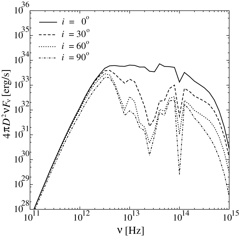
Simulated SEDs are illustrated in Fig. 1. It is seen that SEDs are sensitive to , particularly in the frequency range higher than the peak frequency . This change reflects the asymmetry of the density and temperature distribution. The optical depth along the line-of-sight from an observer to the central star, , is at , while for and for . Thus, for , the dependence on the inclination is within a factor of and the emergent flux is the superposition of the thermal radiation from dust grains, which is determined by the temperature and the total amount of dust, regardless of density distributions. In contrast, for , the anisotropy of flux is very large (2-4 orders of magnitude), and the emergent flux is dominated by the scattered radiation originating from the central star and inner disk, which is strongly affected by the density distribution of the envelope. Therefore, the flux in the pole-on () direction is large, while the flux in the edge-on () direction is small.
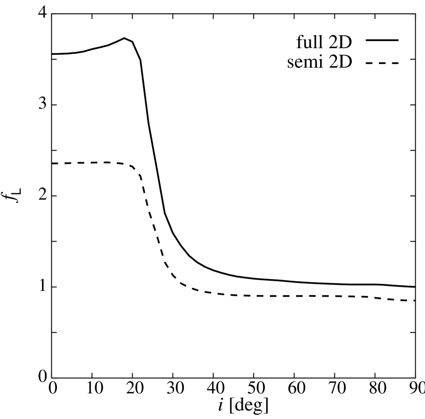
3.3 Comparison between Semi and Full 2D Calculations
To see the importance of full 2D radiative transfer calculations, we performed approximate semi 2D calculations, which were carried out by Kenyon et al. (1993). They derived the temperature distribution in the envelope from radiative equilibrium, but they assumed the spherically symmetric density distribution when they calculated the radiative equilibrium, so they obtained spherically symmetric temperature distribution. To do that, first the spherically averaged density profile from the 2D axially symmetric density distribution is obtained, and then the 1D spherically symmetric temperature profile is calculated. Using the spherical temperature distribution and the non-spherical 2D density distribution, the emergent SEDs from the object are obtained by ray-tracing . Following their procedure, we also calculated the SED from the semi 2D calculations and compared the results with our full 2D calculations.
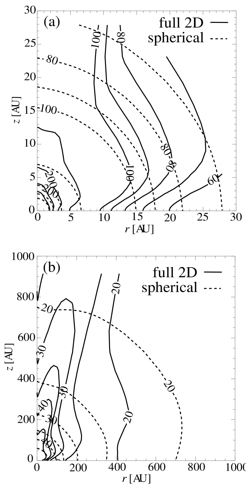
In Fig. 2, we compare two temperature distributions derived from two procedures. The temperature distribution obtained by the full 2D calculations is not spherically symmetric at all. The most noticeable difference between two temperatures is found in the disk and the outflow regions. The temperature in the disk in the full 2D calculation is much lower than that of the spherical temperature, because the disk has higher density than the spherically averaged density. We also find that the temperature in a shaded region, which is behind the disk with respect to the central star, is lower than the spherical temperature, though the density in that region is not so different from spherically averaged one. This is because that the total amount of radiation from the central star to the region is reduced by the efficient disk absorption. In contrast, the temperature in the outflow region in the full 2D calculation is higher than spherical one, because the density in the region is lower than the spherically averaged one. Consequently, it is obvious that the temperature distribution obtained by the full 2D radiative equilibrium calculation is quite different from spherically symmetric distribution.
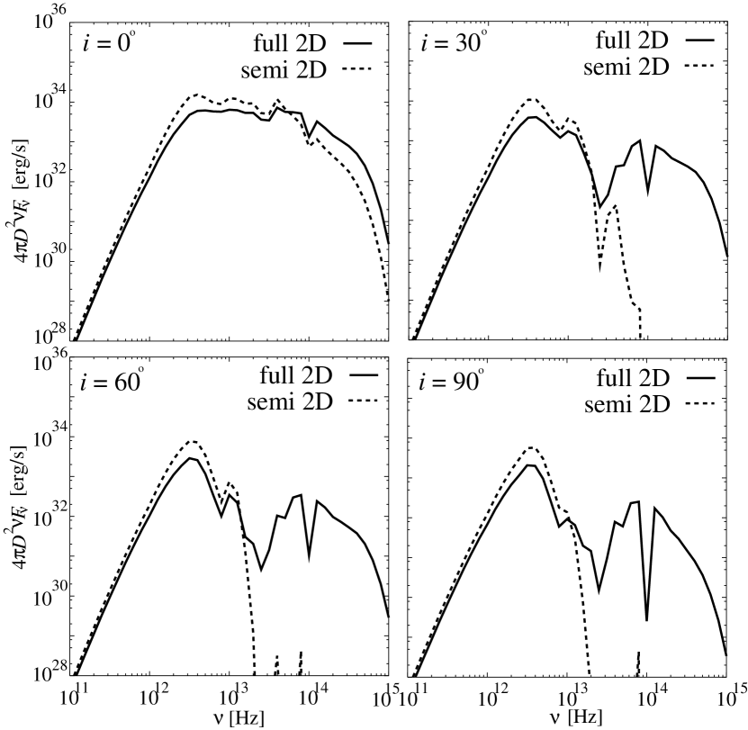
Emergent SEDs based on the temperature distributions displayed in Fig. 2 are shown in Fig. 3. For each inclination, it is seen that (1) the flux derived from the full 2D calculations in a frequency range from to is lower than that of the semi 2D calculations, and (2) in a range from to , the full 2D calculation flux is higher than the semi 2D calculation one. The first difference is due to the decrease of the envelope temperature compared to the spherical temperature. Since the optical depth for the radiation at this frequency from the central star to the observer is around unity, the flux in this range is expected to be in proportion to the dust temperature in the envelope. On the other hand, the second difference is caused by the different mean intensity especially in the outflow region, because flux in this frequency range is mainly determined by the scattering, which is evaluated by , where is scattering coefficient, and is very anisotropic in the non-spherical density distribution cases. We can see from Figs. 2 and 3 that the full 2D radiative equilibrium calculations are indispensable to study the detailed structure of Class 0/I objects using their SEDs and/or images.
4 Estimation of Inclination Angle
4.1 A New Inclination Indicator:
The inclination dependence of SED provides a tool to infer the inclination itself. We introduce the emergent luminosity , which is defined by
| (3) |
as a tracer for the change of SED, where is the distance to the target object and is the observed flux at frequency . Also, using the peak flux (flux at ), we define a ratio by
| (4) |
(Note that , , and are all observable quantities. We can obtain them from observed SEDs.) We show the change of against in Fig. 4. Fig. 4(a) indicates that can be determined if is evaluated from observed SED for the angle of . But, when is in a range , is almost independent of . This means that SED does not change if we observe a protostar through the bipolar cavity. For , is also independent of . It corresponds to the case that we observe a protostar through the disk.
The level of depends on . It implies that is one of the important parameters to determine the anisotropy of a protostar system. The ratio increases for all as increases, and it is worth noting that there exist maximum and minimum of for each .
We calculated for full 2D and semi 2D results shown in Figs. 2 and 3 to clarify the importance of the full 2D calculation. These results are shown in Fig. 5. In the semi 2D calculation, the value of is lower than that of the full 2D calculation, especially for the small inclination. It is because that the peak fluxes are different by a factor of while the difference of observed luminosities is so small. For the large inclination, the differences of and are canceled each other so that the values of are almost the same.
4.2 Test of the Method
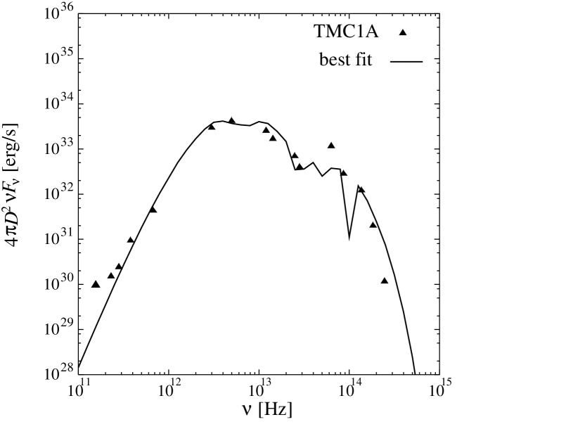
We test our new method with a real object TMC1A (IRAS 04365+2535). TMC1A is a Class I object (e.g. Kenyon et al. 1993; Chandler et al. 1998) and has an outflow with the half opening angle (Chandler et al. 1996; Gomez et al. 1997). According to Motte et al. (2001), TMC1A has an extended envelope and is recognized as a ‘true protostar’ not a ‘transition object’ nor an ‘edge-on view of T Tauri star’. Thus, we think that TMC1A is an archetype of Class I objects and an appropriate example to test our new method to assess the inclination. Observational data of TMC1A are taken from Myers et al. (1987), Kenyon et al. (1993), and Chandler et al. (1998).
Here, we adopt the new method to derive the inclination, and compare the estimate with the results by the full SED fitting. First, we attempt to estimate the inclination of the object using our new method. We evaluate first the observed luminosity by integrating the SED and obtain , which is consistent with the results obtained by Myers et al. (1987) () and Kenyon & Hartmann (1995) (). We next calculate from and , and obtain . From Fig. 4(a), this value indicates that inclination angle is about . This inclination is estimated with our new method only using the and the peak flux, without fitting all the physical parameters of the object.
Next, we try to obtain all the physical parameters of the object by fitting the SED and estimate the inclination angle. In practice, we fit the SED going through the following steps:
-
1.
Set the outflow half opening angle .
-
2.
Infer the luminosity of the central star from the peak flux of the SED.
-
3.
Infer the circumstellar mass (, ) from the flux in a frequency range lower than the frequency of the peak flux .
-
4.
Infer the ratio of the envelope mass to the disk mass and inclination from the shape of the SED in a frequency range higher than .
The best fitted SED is displayed in Fig. 6 and adopted parameters are listed in Table 2. It is seen that our model can reproduce the observational data very well. In this procedure, the inclination of the object is estimated to be .
It is clear that the estimated values obtained by above two different methods agree quite well with each other. Since the estimation based on the full SED fitting is considered to be more reliable, it seems that the new spectrophotometric method provides an effective tool to assess the inclination.
However, it should be noted that the inclination angle obtained above does not agree with the values obtained by Kenyon et al. (1993), which is , and Chandler et al. (1996), . Such discrepancy could be attributed to the method used to infer the inclination. Kenyon et al. (1993) used the spherically symmetric temperature distribution when they estimated the inclination with the SED. But the spherical temperature distribution can lead a significant difference in the resultant SED as shown in section 3.3. Chandler et al. (1996) estimated the inclination angle based on the shape of outflow lobe on the sky. They first restricted the inclination angle to be less than . Then, they placed the lower limit of the inclination to be , though the reason why they adopted the value was not given clearly.
4.3 Effects of Other Parameters
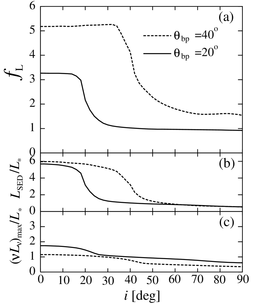
Here, we estimate uncertainties of the present method by changing parameters of the model. As shown in Fig. 4(a), an uncertainty of is large if the half opening angle is thoroughly unknown. But, it is possible to pose a constraint for in the Class I phase by the observation of outflow lobes (Cabrit & Bertout 1986). For example, it is estimated that - for Class I object TMC1 (IRAS04381+2540) and - for TMC1A (IRAS04365+2535), respectively (Chandler et al. 1996). There are also some other results for estimation of : for L1448 (Bachiller et al. 1995) and B335 (Hirano et al. 1988; Chandler & Sargent 1993), and for L1551 IRS5 (André et al. 1990). From these estimations, it seems possible to constrain to be - . This constraint would be justified by the fact that if becomes larger than this range, resultant SED exhibits double peaked feature in far-IR and near-IR to optical, but these SEDs are not classified Class I category. From Fig. 4(a), a typical error for determination of is if we restrict ourselves to - .
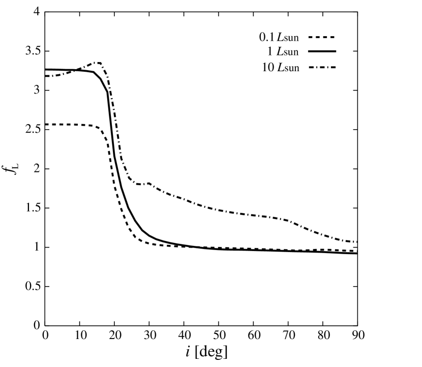
Next, we examine to what extent the luminosity of the central star affects the ratio . Fig. 7 shows calculated as functions of the inclination with three different luminosities, , , and . It is seen that when the luminosity of the central star is low (), for the small inclinations decreases compared to the standard case (), but for the large inclinations does not change. In contrast, when the luminosity is high (), for the large inclinations becomes higher than the standard case, while for the low inclinations remains the standard value. It is true that is affected by the central star luminosity to some extent, but the change of the value in a range sensitive to the inclination is not large. Thus, when we estimate the inclination of an object using this new method and , the effect of the central star luminosity seems to be negligible.
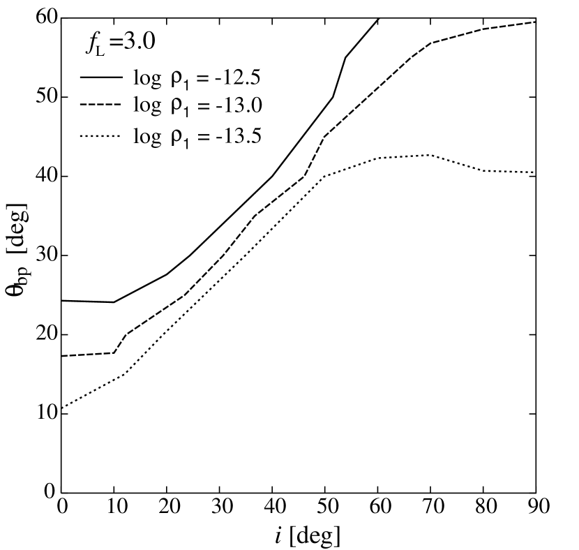
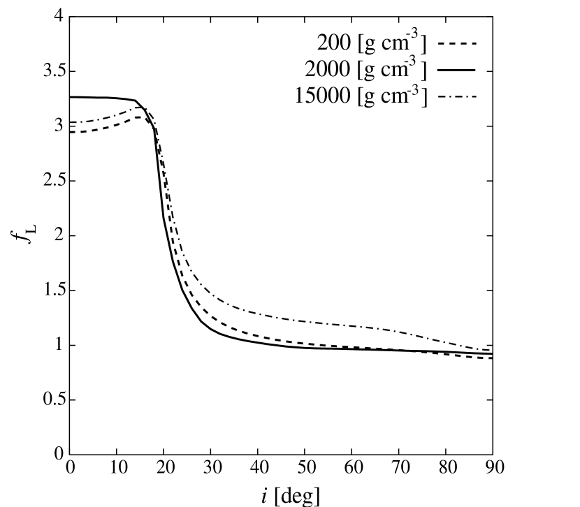
Also, could affect the results. Fig. 8 shows the condition of for each in the plane. The flux at decreases with increase of , because is proportional to and the flux in this frequency range is proportional to . In contrast, the flux at increases with increase of because the total amount of dust grains is increased. Thus, tends to decrease with increase of , so that the line of is shifted above with increasing in the plane. For , the inclination changes by when changes by an order.
By contrast, does not influence . Fig. 9 displays calculated with different . It is easily seen that does not change significantly. This is because the circumstellar disk contribute little to the column density along the line of sight, on which strongly depends.
Therefore, we conclude that the primary uncertainty of our method comes from the information of . If can be estimated by any other means, then the error of inclination obtained by our method becomes roughly . If is unknown, then the error may be roughly .
5 Conclusions
Using 2D radiation transfer calculations, we have obtained the radiation fields for 2D axisymmetric protostar model, consistent with the central star, the circumstellar disk, and the envelope, and derived the SEDs of Class I objects. We have found that the ratio between the emergent luminosity, , and the peak flux in the SED, , is a good indicator of the inclination angle of the object, because is sensitive to the inclination, while the peak flux is insensitive. Through the test with real data and the analysis on the other physical parameters, it has been shown that is a robust tool to assess the inclination of a Class I object. Hence, can provide a new spectrophotometric method to estimate the inclination angle of a Class I object. It is beneficial that, in this new method, only the luminosity and the peak flux are needed to estimate the inclination. The typical error of the method is roughly if the half opening angle is known and roughly if it is unknown.
The present method is applicable for a great deal of data provided by future missions of infrared, sub-millimeter, and millimeter observatories, e.g., SIRTF, ASTRO-F, and ALMA. These missions are expected to reveal numerous protostar candidates. Then, it may be possible to carry out precise statistical study of protostars. The present spectrophotometric method could be a powerful tool in the statistical study.
References
- Adams, Lada, & Shu (1987) Adams, F. C., Lada, C. J., & Shu, F. H. 1987, ApJ, 312, 788
- André et al. (1990) André, P., Martín-Pintado, J., & Montmerle, T. 1990, A&A, 236, 180
- André et al. (1993) André, P., Ward-Thompson, D., & Barsony, M. 1993 ApJ, 406, 122
- Bachiller et al. (1995) Bachiller, R., Guilloteau, S., Dutrey, A., Planesas, P., & Martin-Pintado, J. 1995, A&A, 299, 857
- Cabrit & Bertout (1986) Cabrit, S. & Bertout, C. 1986, ApJ, 307, 313
- Chandler et al. (1998) Chandler, C. J., Barsony, M., & Moore, T. J. T. 1998, MNRAS, 299, 789
- Chandler & Sargent (1993) Chandler, C. J. & Sargent, A. I. 1993, ApJ, 414, L29
- Chandler et al. (1996) Chandler, C. J., Terebey, S., Barsony, M., Moore, T. J. T., & Gautier, T. N. 1996, ApJ, 471, 308
- Gomez et al. (1997) Gomez M., Whitney, B. A., & Kenyon, S. J. 1997, AJ, 114, 1138
- Hayashi, Nakazawa, & Nakagawa (1985) Hayashi, C., Nakazawa, K., & Nakagawa, Y. 1985, in Protostars and Planets II (Tucson: Univ. Arizona Press), 1100
- Hirano et al. (1988) Hirano, N., Kameya, O., Nakayama, M., & Takakubo, K. 1988 ApJ, 327, L69
- Kenyon, Calvet, & Hartmann (1993) Kenyon, S. J., Calvet, N., & Hartmann, L. 1993, ApJ, 414. 676
- Kenyon & Hartmann (1995) Kenyon, S. J. & Hartmann, L. 1995, ApJS, 101, 117
- Kikuchi, Nakamoto, & Ogochi (2002) Kikuchi, S., Nakamoto, T., & Ogochi, K. 2002, PASJ, 54, 589
- Lada & Wilking (1984) Lada, C. J. & Wilking, B. A. 1984, ApJ, 287, 610
- Men’shchikov, Henning, & Fischer (1999) Men’shchikov, A. B., Henning, T., & Fischer, O. 1999, ApJ, 519, 257
- Miyake & Nakagawa (1993) Miyake, K. & Nakagawa, Y. 1993, Icarus, 106, 20
- Motte & André (2001) Motte, F. & André, P. 2001 A&A, 365, 440
- Myers et al. (1987) Myers, P. C., Fuller, G. A., Mathieu, R. D., Beichman, C. A., Benson, P. J., Schild, R. E., & Emerson, J. P. 1987, ApJ, 319, 340
- Nakamoto & Kikuchi (1999) Nakamoto, T. & Kikuchi, N. 1999, in Proceedings of Star Formation 1999, ed. T. Nakamoto (Nobeyama Radio Obs.: Nobeyama), 217
- Shu (1977) Shu, F. H. 1977, ApJ, 214, 488
- Stone et al. (1992) Stone, J. M., Mihalas, D., & Norman, M. L. 1992, ApJS, 80, 819
| Symbol | Meanings | Parameter Range |
|---|---|---|
| luminosity of central star | ||
| temperature of central star | ||
| mass of central star | ||
| surface density of disk at | aaThis corresponds to the disk total mass assuming dust-to-gas mass ratio of . | |
| power law index of disk | ||
| density of envelope at | - bb corresponds to the envelope total mass assuming dust-to-gas mass ratio of and | |
| power law index of envelope | ||
| opening angle of bipolar cavity | - | |
| inclination angle | - |
.
| Object | [] | [g ] | [g ] | KCH | Outflow | |||
|---|---|---|---|---|---|---|---|---|
| TMC1A | 1.0 |