Development of an atmospheric Cherenkov imaging camera for the CANGAROO-III experiment

Abstract

A Cherenkov imaging camera for the CANGAROO-III experiment has been developed for observations of gamma-ray induced air-showers at energies from 10¹¹ to 10¹⁴ eV. The camera consists of 427 pixels, arranged in a hexagonal shape at 0.17^∘ intervals, each of which is a 3/4-inch diameter photomultiplier module with a Winston-cone–shaped light guide. The camera was designed to have a large dynamic range of signal linearity, a wider field of view, and an improvement in photon collection efficiency compared with the CANGAROO-II camera. The camera, and a number of the calibration experiments made to test its performance, are described in detail in this paper.

, , , , , , , , , , , , , , , , , , , , , , , , , , , , , , , , , , , , , , , , , , , , , ,

1 Introduction

CANGAROO (the Collaboration of Australia and Nippon for a GAmma Ray Observatory in the Outback) is a project to study TeV gamma-ray emitting celestial sources, particularly those in the southern sky. The earlier experiments CANGAROO-I and CANGAROO-II, using single telescopes of 3.8-meter [1] and 10-meter diameter, respectively, obtained glimpses of astronomical objects such as pulsars (PSR 1706-44 [2], Crab [3]), active galactic nuclei (Mrk 421 [4]) and supernova remnants (SN1006 [5], RXJ1713.7-3946 [6, 7]).

CANGAROO-III, the next phase of the project, aims at the detection at energies of 0.1$\sim$100 TeV (1TeV=10¹²eV) using four 10-meter-diameter telescopes for stereoscopic (and “multi-scopic”) reconstruction of atmospheric Cherenkov shower images. Various improvements in the design of the imaging Cherenkov camera have been made for the CANGAROO-III experiment [8, 9, 10].

The first telescope of the CANGAROO-III array is the CANGAROO-II telescope, which has been in operation since April, 2000. The telescope has an optically parabolic shape, and consists of 114 small spherical mirrors with diameters of 80 cm and made of carbon-fibre reinforced plastic [11]. The second telescope was built in March 2002 and the remaining two telescopes will be constructed by the end of the 2004.

The technique of stereoscopic observing [12, 13], allows more precise measurements to be made: a significant improvement in the separation efficiency of gamma-ray events from the cosmic-ray background, a more precise reconstruction of the arrival direction determined on an event-by-event basis [14], and an improvement in the energy resolution of up to 20% [15]. The stereoscopic technique is effective for both point-like sources and for extended gamma-ray sources, such as supernova remnants.

Measurement of the gamma-ray energy spectrum over a wide range is important for determining the gamma-ray emission mechanism. Information derived from spectral features, such as the spectral index and any cutoff energy, can help clarify the acceleration and production mechanisms, and also provide estimations of fundamental parameters, such as the magnetic field and the maximum energy of the particles accelerated at the source [5]. For instance, for the Crab nebula, the detection of gamma-rays above 50 TeV is a key to finding the acceleration limit in the pulsar nebula [3]. Also, for supernova remnants, measurement of the energy spectrum at sub-TeV energies has provided evidence for proton acceleration [7]. Spectral measurements are crucial for solving the mystery of the origin of cosmic rays.

Another goal of the experiment is to extend observations into the energy region between $\sim$10 GeV (below which was explored by the EGRET detector on the Compton Gamma-Ray Observatory [16]) and the typical Cherenkov telescope threshold to date of 200–300 GeV. A number of the astronomical objects observed by EGRET are expected to be detectable with Cherenkov telescopes by narrowing this gap. A lowering of the energy threshold will also allow the detection of new gamma-ray sources, especially those with steep energy spectra, such as distant active galactic nuclei, for which sub-TeV gamma-rays are less attenuated by the infrared background than those in the TeV region [17, 18, 19].

In this paper, the development of the Cherenkov imaging camera for the second CANGAROO-III telescope is described. Detailed studies were made concerning the number, size, type and arrangement of photomultiplier tubes, the preamplifier circuits, the light guides, reliable calibration sources and the overall performance of the camera system.

2 Miscellaneous developments

The weight of the camera was constrained by the mechanical structure of the telescope to be less than $\sim$100 kg. Based on a structural analysis, a deformation of $\lesssim$2 mm at the focal plane would be expected for a 100 kg camera.

Images of gamma-ray showers are located in the focal plane at distance of up to $\sim 1.5^{\circ}$ from the source position. For stereoscopic observations, some refined observation modes have been proposed, such as a “raster scan” tracking mode, with which the telescope tracking centers simultaneously scan a square region of $\pm$0.5^∘ in right ascension and declination coordinate centered on the target [20], a “wobble” mode in which the telescopes are pointed at a direction displaced from the source by first $\sim 0.5^{\circ}$ and then $\sim-0.5^{\circ}$ [21], and a “convergent” mode [22]. The field of view of the CANGAROO-II telescope was $\sim$2.7^∘, however from a consideration of the points above we have chosen a wider field of view, $\sim 4^{\circ}$, for the remaining CANGAROO-III telescopes.

Differentiation of gamma-ray and cosmic-ray showers is based on the shape and orientation parameters of the images, such as $length$, $width$, $distance$ and $alpha$ [23, 24]. These are calculated from the amplitudes of the signals detected by the pixels in the focal plane. In order to accurately reconstruct the shower image, good imaging performance, with negligible cross-talk between the pixels and uniform gains for all of the pixels, is required. Also, as a camera with a wider field of view has an increased chance of having a bright star within the field of view, the high voltages (HV) of the camera pixels should be individually controllable, to avoid possible deterioration of photomultiplier tube performance by the higher trigger rates that bright starts cause.

Gamma-ray cascades, which develop in the upper atmosphere, produce light pools with radii of about 120 meters on the ground with a temporal spread of about 10 ns. A high-sensitivity photomultiplier tube (PMT), having a gain (after pre-amplification) of $\sim 2\times 10^{7}$, and some sensitivity to ultraviolet photons, is a suitable detector of Cherenkov photons. It should also be robust and stable, particularly with regard to the night sky background (NSB), since a significant, and time-variable, number of photons are received from the night sky, starlight, and terrestrial sources. A wide dynamic-range, from 1 to 250 photoelectrons (p.e.) with less than 10% deviation from linearity, for each sensor is required for precise measurements of energy spectra. Also, maximizing the collection efficiency of Cherenkov photons is required to reduce the energy threshold.

A timing resolution of less than 1 ns is important for discriminating Cherenkov photons of air showers from the NSB, and is also crucial for the event discrimination of gamma-rays from hadrons using relative arrival time information [6].

3 Camera design

3.1 General design

The camera design of the second CANGAROO-III telescope was made based on the above requirements. A schematic diagram of the camera structure is shown in Fig. 1.

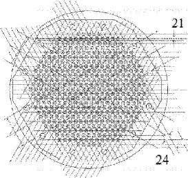
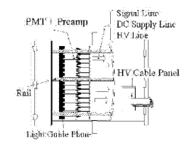
Figure 1: Schematic design of the CANGAROO-III camera frame. The upper figure shows the front view and the lower figure shows a side view of the camera. The camera pixels are arranged on a hexagonal grid, as shown in the upper figure.

The camera is contained in a cylindrical vessel of 800 mm in diameter and 1000 mm in length, which provides shielding from both rain and light. The vessel is made of an aluminum alloy (A5052) in order to reduce the weight and provide sufficient rigidity. Inside the camera vessel, 427 PMT modules, regulator circuit panels, an LED (light emitting diode) light diffuser for gain calibration, and several other instruments such as a thermometer, are contained. Twisted-pair cables for transmitting signals and multi-wired cables for the high-voltage supply are fed into the camera vessel.

The camera frame consists of two aluminum templates (5 mm in thickness), in which holes (21 mm in diameter) are drilled at locations corresponding to each of the 427 pixels, as shown in Fig. 1 (upper). Every PMT module, consisting of an PMT and a preamplifier (20.5 mm in diameter), is held by these templates. Light guides are attached to the front panel. The photocathode plane of the PMT module is held close to the back plane of the light guide. The front panel, on which the light guides are attached, is fixed at the focal plane. All segmented mirrors can be seen from every pixel position.

The pixels are arranged in hexagonal shape in order to maximize the collection efficiency of the Cherenkov light. The pixel size was determined to be 0.17 degrees from a simulation study [13], taking into account the spot size of the 10 m composite mirror [11]. The simulation code was based on GEANT 3.21. It included the electro-magnetic shower and the telescope optics.

3.2 Photomultiplier module

A photograph of the PMT module is shown in Fig. 2.

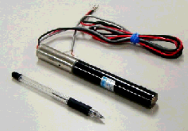
Figure 2: Photograph of the PMT module.

It is cylindrical with a diameter of 20.5 mm and length of 173.5 mm. Three types of cable (the signal, the D.C. power and the high voltage supply) are passed through from the back end of the module. The module consists of a 19 mm (3/4 inch) PMT (Hamamatsu R3479UV), bleeder circuits and a pre-amplifier which are attached at the base of the PMT. An operational amplifier (MAX4107) is used as the pre-amplifier and the input signal from the PMT is amplified by a factor of 60. The bleeder circuit is coated with epoxy resin in order to prevent humidity-related effects. Each module is shielded with $\mu$-metal (0.2 mm thick) to reduce any effect due to the geomagnetic field and cross-talk between PMT modules. Each module (without cables) weighs 75 g.

3.2.1 Photomultiplier tube selection

The 19 mm diameter PMT (15 mm diameter photocathode) was chosen considering the field of view the camera. It meets the requirements of:

• a high sensitivity for light at ultraviolet wavelengths,

• a gain (before pre-amplification) of greater than 10⁵,

• a transit time spread (T.T.S.) of less than 1 ns,

• a wide range of the linear response for 1$\sim$300 photoelectrons with less than 20% deviation from linearity,

• a good signal/noise separation and possible identification of the single photoelectron peak, and

• a light weight and compact size.

Three types of 19 mm PMT (Hamamatsu R1450, R3479 and R5611), shown in Fig. 3, were compared for selection.

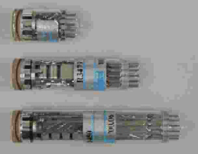
Figure 3: Performance tests were made for three types of 19mm (3/4 inch) diameter photomultiplier tubes (PMTs). The model numbers are, from top to bottom, Hamamatsu Photonics R5611, R3479 and R1450, respectively. The R3479 was selected for the CANGAROO-III PMT module.

The basic characteristics of these PMTs are listed in Table 1.

Model no.	R1450	R3479	R5611
Dynode structure	LINE	LINE	CC
No. of dynode stages	10	8	8
Dynamic range (p.e.)	$>$150	$>$150	50
Weight (g)	19	15	9
Length (cm)	8.8	6.5	3.0
Supplied high voltage ($8\times 10^{5}$ gain)	1170	1500	780
Rise time (nsec)	1.8	1.3	1.5
Transit time (nsec)	19	14	17
Transit time spread FWHM (nsec)	0.76	0.36	0.8

Table 1: Comparison of the performances of three types of PMTs. LINE means linear-focused type of dynode and CC means circular-cage type.

The R5611 has a circular-cage dynode, which is superior in compactness and lower voltage operation, whereas the R3479 and R1450 have linear-focused dynodes. All are light weight, with fast T.T.S.s, and allow the identification of a single photoelectron peak. The choice of PMT was ultimately based on the linear response over a wide dynamic range.

Linearity was checked using a blue LED (NSPB510S, Nichia, $\lambda\sim 470$-nm) [25] which was flashed with a 20 ns wide pulse from a pulse generator (AVI-V-C-N, AVTECH). The high-voltage supplied to each PMT was adjusted to give a gain of $2\times 10^{5}$, which was determined by measurement of the single p.e. peak.

The amount of light was changed in the range of $1\sim 250$ p.e. using combinations of neutral density (ND) filters (MAN-52, SIGMA Koki Optical Instruments) with different transmission efficiencies. The optical attenuation of each filter was checked to be within $\pm$1% accuracy. The signal outputs were amplified by 10 and then digitized by a charge-integrated ADC (Analog-Digital-Converter) (0.24 pC/ch) with a 100-ns gate width. Here, we used a commercial amplifier of PHILLIPS (model 776). Its linearity was checked in advance. Trigger signals were made using the output signals of the pulse generator.

The measured linearities, ADC counts and deviations from linear response as a function of the number of input photons, are shown in Fig. 4.

Figure 4: ADC counts (upper) and deviation from linear response (lower) as a function of number of input photoelectrons. In the lower figure, the large errors at a small input p.e. are considered to be due to the uncertainty in the input number of photoelectrons.

The circular-cage type (R5611) was found to have less linearity at a higher levels of incident light. This is due to the characteristics of the wire structure of the anode (space-charge limitation). Meanwhile, the linearity of the R3479 shows a slightly better result than that of the R1450. From this result, and also the considerations of compactness and weight, the R3479 was determined to be the most suitable for our experiment,

UV glass, which has a better transparency for ultraviolet wavelengths, is used for the photocathode window. The quantum efficiency is discussed further in section 4.1.4.

3.2.2 Preamplifier circuit

The characteristics of a fast rise-time and a high band-width are required for the preamplifier for signal amplification. Before designing the preamplifier circuit, three types of the preamplifier chips, CS510S (Clear Pulse) [26], $\mu$pc1664c (NEC) and MAX4107 (MAXIM), were tested, to study in particular the linearity of the gain.

The results of the linearity measurement are shown in Fig. 5.

Figure 5: Linearities for three types of preamplifier chips (CS510S, $\mu$pc1664c and MAX4107).

Here, we used R3479 for input of the preamp without the $\times$10-amplifier. The amount of input light was adjusted by combinations of ND filters, as in the previous measurement. From Fig 5, it is found that MAX4107 has the widest dynamic range of the three tested, and so it was selected for the photomultiplier module.

A schematic diagram of the preamplifier circuit is shown in Fig. 6.

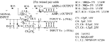
Figure 6: Schematic diagram of the preamplifier circuit.

The feedback resistances are selected by adjusting the proper gain of the preamplifier. The rise time of the pulse signal is smeared to $\sim$5 ns at the signal input (C3 in Fig. 6) to simulate transmission in the signal cables. As the duration of the Cherenkov light from air showers is of the same order, this smearing has the advantage of reducing the peak voltage of the signal, allowing a wider dynamic-range of the linearity to be obtained.

3.2.3 High-voltage polarity

The positive polarity of the high voltage is supplied to the PMTs (cathode-ground). The advantage of a cathode-ground is that it prevents discharges between the cathode plane of the PMT and the metal structure of the camera. The light-guide can be attached directly at the photocathode plane of the PMT module.

In the CANGAROO-II camera [27], a polycarbonate light-guide was attached to the PMT window where the negative polarity is applied (anode-ground). Frequent discharges were observed on nights of high humidity (especially in winter). Some space ($\sim$2 mm) between the photocathode was required, which significantly decreased the collection efficiency. Also, this HV configuration was found to be the cause of an increase in the noise rate at the single-photon level because of an instability of the electric potential, as shown in the following measurement.

Fig. 7 shows the noise count rates of the PMT for the following setups:

Setup 1:

reference measurement, with nothing near the PMT window,

Setup 2:

a grounded copper tape attached to the PMT window,

Setup 3:

a polycarbonate light-guide, with a surface which was deposited by aluminum vapor and coated by silicon oxide, was attached to the PMT window, but electrically isolated from the ground level,

Setup 4:

the light-guide was attached to the PMT window, and grounded, and

Setup 5:

re-measurement of Setup 1, for confirmation.

Figure 7: Count rates for different PMT setups. The filled marks (circles, squares and triangles) show the results with the anode-ground setup (negative polarity of the supplied voltage), and the open marks show that of the cathode ground (positive polarity). See text for details of the setups.

The PMT was placed in a light-tight box and the noise rate measured with a threshold discrimination of $-20$ mV, corresponding to the single-photoelectron level. For each setup, both the cathode- and anode-ground were tested three times. It was found that setups 2 and 4 with the anode grounded showed the highest noise rate, while the noise rate for all cathode-grounded cases was stable. This shows that the electrical stability of the cathode plane is important for the PMT noise rate.

A minor disadvantage of the cathode-ground setup is that signal extraction from the PMT anode must be done with an AC coupling, i.e., it prevents us from measuring the DC current at the PMT anode. However, this is not an important consideration as the threshold level of the pulsed photons is constant because the DC level of the preamplifier input becomes stable around the ground level under any circumstance. Also we monitor a single trigger rate for each PMT by scaler circuit (in each second with 700 $\mu$s timing gate). It helps us to know the background light level.

3.2.4 High-voltage bleeder

A schematic diagram of the high-voltage bleeder circuit is shown in Fig. 8.

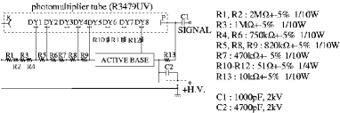
Figure 8: Schematic diagram of the high-voltage bleeder.

An active base, which stabilizes the electric potential difference between the dynodes, was introduced at the 6th to 8th locations of the dynodes. This is to prevent any deterioration of the dynode amplification when the bleeder suffers from a high constant current flow due to a huge background of photons, such as the effects of a bright-star effect (magnitude $<$3).

Precise and stable measurements of the pulse height are necessary even under a wide variety of background photon rates. The feasibility of a photon pulse measurement was investigated for several conditions under various background photon rates. Fig. 9 shows the difference in the pulse height for different levels of background photon fields.

Figure 9: PMT gains for different amounts of background photons. The upper figures show the measurement for the anode-ground (left) and the cathode-ground (right) setup for PMTs which were not equipped with active base dynodes. The lower figures show the cases for the PMTs equipped with an active base.

When the incident light level exceeds a certain level, the anode current began to deviate from the ideal linearity. The detail of this phenomenon can be found in Ref. [28]. The typical night-sky background is estimated to be $2.6\times 10^{-4}$ erg/cm²/s/str [29]. Therefore, a single photoelectron rate of $\sim$17 MHz for each pixel is expected from background photons when the camera is installed at the focal plane of telescope. We carried out tests with up to 15 times more photons than this typical background and for both cathode- and anode-ground. From these results, the gain of the PMTs which had active base dynodes, was found to be stable under an environment of severe background photons.

3.3 Light-guide

The camera consists of PMTs with a significant amount of dead space between them, amounting to $\sim$65% of the total surface area. Light-guides reflect photons which would otherwise be incident upon the dead space onto the photocathode area of the PMTs, thus increasing the light-collection efficiency. Another advantage is that light-guides reduce the background of photons coming from outside of the mirrors, i.e., at a shallow angles with respect to the light-guide plane.

After Monte Carlo simulations for various shapes of light guides were performed to evaluate their performance, the optimal shape of the light guide was determined. The most efficient light guide design was based on the Winston cone, but with a hexagonal entrance shape.

3.3.1 Shapes of light guides

Various types of light guides made by combining the Winston cone, paraboloids and flat planes were examined by simulations. The Winston cone is a non-imaging optical shape used to concentrate all photons whose incident angle is less than a certain angle [30, 31]. The maximum incident angle to the light guide is determined by the incident light from the outer edge of a 10 m mirror dish, which ranges from 32.2^∘ to 35.2^∘, depending on the position of the camera surface. Although the entrance shape of the original Winston cone is round, as the PMT’s are arranged on a hexagonal grid with a spacing of 24 mm, a hexagonal entrance aperture was chosen so as to obtain less dead space and a better light-collection efficiency. The ratio of the entrance area and the exit area of the light-guides is 2.68 for the case of a gap of 0 mm between the light-guides and 2.46 for a 1 mm gap.

3.3.2 Light-collection efficiencies

Simulations to obtain the light collection efficiency were carried out based on the following simplified assumptions:

1. The diameter of the sensitive area of the PMT is 15 mm.

2. The distance between the centers of neighboring PMTs is 24 mm.

3. Reflectances of 100% and 80% were trialled for the surface of the light-guide.

4. The reflectance at the surface of the PMT is assumed to be 0%.

5. Gaps of 0 mm and 1 mm were trialled between neighboring light-guides.

6. Gaps of 0 mm and 2 mm were trialled between the light-guide and the PMT surface.

7. Photons are illuminated on the paraboloidal 10 m mirror and reflected at the mirror surface; they are then injected on a light guide centered at the camera position.

8. The camera position is assumed to be at the focal plane, 8 m in front of the main reflector.

The simulations showed that, as expected, the collection efficiencies varied as the light-guide shape was changed. For example, efficiencies between 69.4% to 77.3% were obtained for a reflectance of 80%, and gaps of 0 mm. The best case was obtained for a shape for which every cross section through the central axis had the shape of Winston cone.

The effects of the gap between the light guides, the gap between the lightguide and the PMT surface, and the reflectance of the light guides are given in Table 2.

Gap between LGs	0 mm	1 mm
Reflectance of LG : 100 %
Gap between LG and PMT : 0 mm	94.3 %	87.0 %
Reflectance of LG : 80 %
Gap between LG and PMT : 0 mm	77.3 %	72.2 %
Reflectance of LG : 80 %
Gap between LG and PMT : 2 mm	69.0 %	66.4 %

Table 2: Simulated light-collection efficiencies for various cases.

It was found that only a 2mm gap between the lightguide and the PMT surface reduces the efficiency by nearly 10%.

Based on these results, we again chose a design for which the cross-sections were Winston cones, the entrance shape was hexagonal, and the exit shape was round. A mold was turned with a computer-controlled machine based on the data shown in Fig. 10, and finally polished by hand.

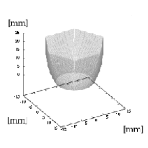
Figure 10: Data points of the inner shape of the new light guide.

Polycarbonate plastic was used for the base material. A picture of the final product is shown in Fig. 11.

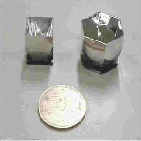
Figure 11: Left : Light guide for the CANGAROO-II telescope.     Right : New light guide for the CANGAROO-III telescope. The coin shown is 26 mm in diameter.

The manufacturing error of the size was measured and proved to be less than 0.1 mm, however, as there is likely to be some temperature dependence, a more conservative value 0.5 mm was chosen for the gap between light-guides. Aluminum vapor was deposited on the inner surface of the light guide and the surface was then coated with silicon oxide.

The light-collection efficiency was measured for the manufactured light-guide as a function of the incident angle using a blue LED with a wavelength of 470 nm. Figure 12 shows the measured efficiency, which agrees very well with a simulation when the reflectance of the inner surface was assumed to be 89%.

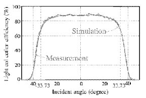
Figure 12: Comparison of light collection efficiency between a simulation and a measurement of the light-guide.

3.3.3 Reflectance vs. wavelength

Small flat glass samples were put in the same vessel for vapor deposition with light-guides. The reflectance of the samples was measured by a spectrophotometer. One of the results is shown in Fig. 13 as a function of wavelength.

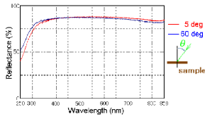
Figure 13: Measured reflectance of the new light-guide.

The incident angles for this measurement were 5^∘ and 60^∘. The reflectance value ranges from 75% to almost 90% above a wavelength of 310 nm for both incident angles.

The light-collection efficiency of the light-guide for the camera of the second telescope of CANGAROO-III was improved by about 60% compared with that of the first (CANGAROO-II) telescope. The negative high voltages applied to the first telescope camera caused discharge problems if the light guides were directly attached to the PMTs. Avoiding this problem requires keeping gaps of about 2 mm between the light guides and the PMTs, which reduces the light-collection efficiency considerably. The second telescope camera employs a positive high voltage to prevent any discharge, and so that light guides can be attached directly to the surface of the PMTs.

Because the Winston cone shape is used, the light-collection efficiency of the new light guide drops rapidly at around 35^∘ (Fig. 12), which corresponds to almost the edge of the 10 m mirror, whereas that for the first telescope changes much more slowly. Background photons coming from outside of the mirror will also be suppressed very much by this property, which will help reducing the trigger rate. Overall, the light-collection efficiency has been greatly improved with the new design for the light-guide.

3.4 High-voltage supply

A multi-channel and individually controllable high-voltage supply system is required in order to obtain a uniform pixel gain. The high-voltage supply system (CAEN SY527) controls up to 10 modules of CAEN A932AP, each of which contains 24 channels of the voltage supply. The primary voltage of the board can be changed over the range of 0–$2550$ V and the voltage for the respective channel can be adjusted independently over the range of $-900$–0 V from the primary voltage, in 0.2 V intervals.

This high-voltage system can be programmably controlled via the VME module, CAEN V288. A computer-displayed control program was constructed using a Tcl/Tk graphical interface, making it possible to monitor the status and to control the supplied high voltage. Also, the monitor program can calculate the position of a bright star image on the camera plane using the SAO (Smithsonian Astrophysical Observatory) catalog and accordingly control the gain of the corresponding pixels on a timescale which is much faster than the passage of the bright stars around the field of view ($\sim$30 s/pixel).

3.5 D.C. voltage supply for a preamplifier

DC voltages ($\pm 5$ V) are supplied to the preamplifier circuits. In order to reduce the voltage drop due to the cable loss (247 $\Omega$/km, i.e. 6.7 $\Omega$ for 27 m), the voltages are regulated at the regulator boards located inside the camera vessel. The basic voltages are derived from front-end modules located in an electronics hut with $\pm 12$ V [9] and transmitted through twisted-pair cables.

Each regulator board provides voltages for 16 channels. A DC noise filter was introduced to reduce the noise due to oscillation via the 27 m cables. A DC fan (size 20$\times$20 mm) is attached to each regulator chip in order to keep temperature variations on the regulator board to within 5^∘C. The noise due to this fan on the output signal was observed to be negligibly small.

3.6 Cables

The total weight of the cables should be less than 70 kg in order to minimize the deformation of the camera supporting stays, i.e., to keep the focal plane center within 2 mm. Therefore, multi-wire cables were selected instead of coaxial cables to transfer signals and to supply high voltages; 29 twisted-pair cables, 27 meters in length, and 20 multi-wired cables, 33 meters in length, were bound to the supporting stays and connected to the camera vessel. Each twisted pair cable contains 20 pairs. The signals from the 16 PMT modules are brought together into one twisted-pair cable and transferred to the front-end module at the electronics hut [9]. The remaining 4 pairs are used to transfer the DC power for the preamplifier circuits. The weight of the cables amounts to 130 g per meter. The rise time of the pulse signal is broadened by the cables to $\sim$5 ns, but this effect was taken into account in the preamplifier circuit, as described in section 3.2.2.

High voltages are supplied through multi-wired cables 33 m long and weighing 150 g per meter. Twenty-four channels can be supplied with one multi-wired cable. In addition, two coaxial cables (58C and 174/U), an ethernet cable, and the AC power supply cables, are also fed into the camera vessel.

3.7 Calibration light source

Calibration measurements during an observation are important for precise determinations of the properties of gamma-ray showers. These are carried out by two methods. The uniformity and absolute value of the gain, and the time jitters of the signal pulses, are calibrated using the following light sources.

3.7.1 Distant LED light source

The relative-gain uniformity and the timing jitter of the pulse signal are calibrated using light from an LED; the amount of light and the timing are uniformly distributed at the focal plane. The LED is mounted at the center of the telescope dish, 8 meters from the focal plane. A blue LED (NSPB510S, Nichia), which emits light of $\sim$470 nm in wavelength, is used. The light from the LED is oriented about 30^∘ from the optical axis so that it can be diffused by an optically frosted glass. The uniformity of the light source on the camera plane was measured to be 1.7% using a CCD (ST-5C, SBIG) in the laboratory.

The advantage of this calibration method is that the data can be taken during an observation without changing the experimental setup, and so the effect of the background photons due to the night sky can be taken into account. The disadvantage of this method is that we can not see a single photoelectron peak under the huge night-sky background.

3.7.2 LED system in the camera vessel

To monitor the gain of the whole camera system over the longer term, a new compact monitor system was developed for the camera vessel, consisting of an LED and a specially patterned screen to diffuse the light uniformly to every pixel. The absolute number of photoelectrons by the PMTs can be calculated from the widths of the distributions of the output charges from the PMTs based on Poisson fluctuations. Using this device and method, the gain of every PMT can be obtained precisely. The high uniformity of light over the camera surface has the advantage of reducing the calibration time. As this device is used when the camera lid is closed, these operations can be carried out even during the day.

The calibration unit consists of a patterned screen and a LED box containing a blue LED (NSPB520S, Nichia), a reflector, and optical diffusers (shown in Fig. 14).

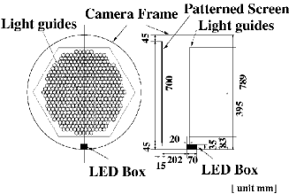
Figure 14: Conceptual figure of the camera LED system, which consists of a light source (LED box) and a patterned screen installed in the camera vessel.

The reflector was painted with white VH enamel to diffuse the LED light uniformly; the diffusers were made of opaque white plastic. The patterned screen is placed 22.2 cm in front of the light-guides, and is attached to the camera lid. The screen is made of polystyrene foam and pattern-printed plastic sheets (70 cm in diameter and 1.5 cm thick). Black squares 1mm² in area are printed on the reflector sheet with a graded density to achieve a uniform distribution of light over the camera. The sheet design was based on a Monte-Carlo simulation, initially assuming that white sheets reflect all incident light and that the black toner absorbs it completely, and taking into account the positions of the light source and the screen, and the solid angle dependence from the light source. The sheets were printed out on a monochrome laser printer. After measuring the light intensity of the screen illuminated by the actual light source, the measured data were fed back into the simulation. This procedure was repeated iteratively until good uniformity was obtained. The final pattern is shown in Fig. 15.

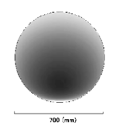
Figure 15: The patterned screen used to obtain a uniform light intensity across the camera from a single LED located at the bottom of the screen.

The light intensity measured by a single PMT whose position was computer controlled with an accuracy of about 0.1 mm on an X-Y stage over an area of 20 cm $\times$ 40 cm, as shown in Fig. 16.

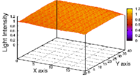
Figure 16: Light intensity at the surface of the patterned screen over an area of 20 cm $\times$ 40 cm. The average deviation from uniformity was measured to be 2.6%.

The average deviation from uniformity of the light intensity was 2.6%.

The average number of photoelectrons ($\mu_{p.e.}$) can be obtained from the ADC distribution, assuming it obeys a Poisson distribution, where we assumed that the ADC counts are proportional to the generated number of photoelectrons. The Poisson distribution satisfies the following formula:

$$\mu_{p.e.}=\biggl{(}\frac{{\mu_{ADC}}}{{\sigma_{ADC}}}\biggl{)}^{2},$$ (1)

where $\mu_{ADC}$ and $\sigma_{ADC}$ are the average values of the distribution of ADC counts and its standard deviation, respectively.

The linearity of the whole camera system for 427 pixels is measured by this method. The number of photoelectrons derived using the above formula is plotted as a function of the ADC counts in Fig. 17.

Figure 17: Obtained number of photoelectrons as a function of the average ADC counts. A straight line fits the data well.

These points are well fit by a straight line at high input photons. The deviations of the measured data points from the fitted line is shown in Fig. 18.

Figure 18: Deviation of data from the fitted straight line.

The deviation is found to be within 2% from 10 p.e. to 50 p.e.. The larger deviations observed for smaller numbers of photo-electrons was caused by the finite resolution of the PMTs.

4 Calibration

4.1 Calibration of each PMT

Before the camera was constructed, the characteristics of all PMT modules were calibrated individually and the results were stored in a database. The following properties of the 450 PMT modules, including reserves, were calibrated:

• high-voltage dependence of the gain,

• linearity from 1 to 1000 p.e.,

• timing resolution, and

• quantum efficiency.

The calibration system was set up to be similar to the actual experiment, i.e., the output signal was passed through a twisted-pair cable of the same length in order to take into account the effects due to the cable loss and the deterioration of the rise time.

The output signal was split into two, with one signal converted by a charge-integrated ADC with 12 bit resolution and with 1 count corresponding to 0.24 pC, and the other signal fed into a TDC of 24.4 ps resolution. Pulses with a width of 20 ns were sent to the LED, and the amount of light was roughly adjusted by changing the supplied voltage. Various amounts of light input were able to be distributed using combinations of neutral density (ND) filters of various transmittance.

The 450 PMT modules were calibrated by the following procedure:

1. The HV was adjusted to give a gain of $1.2\times 10^{7}$ (including the preamplifier gain), to measure the single-photon spectrum.

2. The amount of the light was changed to be 1, 10, 50, 100, 210, 280, 350, 500, 700, and 1000 p.e..

3. The high-voltage dependence of the gain was measured with the amount of 10 p.e. input.

Fig. 19 shows the typical distribution of a single photoelectron peak.

Figure 19: Distribution of the single-photoelectron peak measured by a PMT module.

The peak due to a single photon signal can be clearly separated from the background. Through these calibration processes, five of the 450 PMT modules were rejected as they did not meet at least one of the following requirements.

4.1.1 Gain linearity

Fig. 20 shows the linearity of all the PMT modules for gain (including pre-amplification) of $1.2\times 10^{7}$.

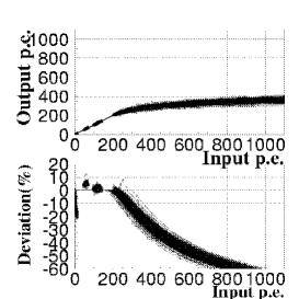
Figure 20: Fitted curves (upper) and deviations from the linear response (lower) for all PMT modules.

Data points were fitted using the following empirical formula:

$$F(x)=\left\{\begin{array}[]{@{\,}llll}x&&&\mbox{($x\leq a$)}\\ \frac{((x-a+c)^{b}-c^{b})}{b}c^{(1.0-b)}+a&&&\mbox{($x>a$)},\end{array}\right.$$

where $a$ approximately corresponds to the turning point of the line. The resulting average and standard deviation of $a$ were $202.1\pm 12.7~{}(1\sigma)$ p.e., as shown in Fig. 21 (upper).

Figure 21: Distribution of the parameter $a$ (upper) for all PMT modules and the deviation from the linearity at 250 p.e. of the input photons (lower).

The deviation from a linear line at 250 p.e. of the input light was estimated to be $-5.1\pm 2.0~{}(1\sigma)$ % from Fig. 21 (lower). PMT modules with a deviation worse than $-$20% were rejected.

4.1.2 High-voltage dependence of gain

Fig. 22 (upper) shows the high-voltage dependence of the gain.

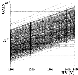
Figure 22: The upper figure shows the gain versus high voltage for all PMT modules. The data points were fitted with the function $K\cdot V^{\alpha}$. The lower figure shows the distribution of parameter $\alpha$, obtained from the fitted line.

The gain was measured at HVs of 1100, 1200, 1300, 1400 and 1450 V, and fitted to the following formula:

$$(\mbox{Gain})=K\cdot V^{\alpha},$$

where $V$ is the supplied high voltage and $K$ and $\alpha$ are free parameters. The parameter $\alpha$ represents the gain sensitivity for the high voltage, and the average value for all modules was $4.9\pm 0.1$, as shown in Fig. 22 (lower). PMT modules with $4.5<\alpha<5.25$ were selected in order to keep the operating HV within the controllable range. Using these fit parameters, it is possible for observations to be conducted with the appropriate gain achieved by changing the HV according to the values in the database.

4.1.3 Timing resolution

The timing resolution of each PMT module was estimated after a correction for the time-walk effect. The discrimination timing can be solved analytically when the shape of the signal pulse is approximated by a Gaussian distribution, $\exp(-at^{2})$ and the timing correction can be applied according to the following formula:

$$\mbox{T}_{\mbox{start}}=\sqrt{b\log(\mbox{ADC})-c}.$$

About 10,000 events were obtained for each measurement, and the parameters $b$ and $c$ were obtained by the fitting procedure. For a few PMTs, full measurements were carried out, and each PMT was confirmed to have less than a 1 ns time resolution. When the input signals were greater than 20 p.e., this correction became unnecessary. Therefore we undertook the rest of the time-resolution measurements with a 20 p.e. input (and without the time-walk correction) for the remainder of the PMT modules.

The resulting timing resolution for all PMT modules is shown in Fig. 23.

Figure 23: Timing resolution for 450 PMT modules when 20 p.e. were irradiated.

The average value was $0.96\pm 0.09$ ns. It should be noted that this resolution was obtained under the effect of a deterioration of the rise-time due losses in the 27-meter cable.

4.1.4 Estimation of the quantum efficiency

The quantum efficiencies were measured for 10 of the 450 PMTs as a function of the wavelength, as shown in Fig. 24.

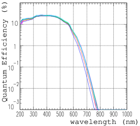
Figure 24: Quantum efficiency as a function of the wavelength measured for 10 PMTs.

The efficiency curves were very similar for all 10 PMTs. Since it is difficult and expensive to measure the quantum efficiency for many PMT modules, the quantum efficiencies were estimated for all modules from the $Skb$ parameter, which gives the sensitivity of the cathode for blue light. $Skb$ was measured with light from a Tungsten lamp filtered with an optical filter to a narrow wavelength band around 400 nm. Its unit is [A/lm]. It is easier to use $Skb$ than to measure the quantum efficiency. We confirmed that there is a good correlation between the quantum efficiency at 400 nm and $Skb$ for the 10 PMTs for which full measurements were made, and then estimated the quantum efficiency based on the measured $Skb$ and the relation derived from 10 PMT sample, which is shown in Fig. 25.

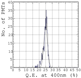
Figure 25: Estimated quantum efficiencies using $Skb$ values.

The average of the quantum efficiency was estimated to be $25.0\pm 1.4$% (a variation of 7.3%).

4.2 Performance of the whole camera system

The total performance of the camera was measured in the laboratory before it was moved to the experimental site. The blue LED calibration source described in section 3.7.1, was placed 8 m in front of the camera. The camera vessel was fixed at two positions of the mounting frame, and was tilted over the range of $0^{\circ}\sim 50^{\circ}$.

High voltages were supplied so as to obtain gains after pre-amplification of $1.2\times 10^{7}$ according to the database derived from the calibrations described in section 4.1. These measurements were made to check:

• the uniformity measurement of the gain,

• the incident-angle dependence of the acceptance efficiency, and

• cross-talk effects.

4.2.1 Uniformity of gain

The uniformity of the gain for all pixels was measured with the diffused LED light source described in section 3.7.1. The amount of incident light to each pixel area was adjusted to be about 50 p.e. The uniformity of the light is described in section 3.7.1.

Fig. 26 shows the uniformity of the gain for all PMT modules.

Figure 26: Gains for all PMT modules in the camera.

We should note that the measured gain by this calibration should be slightly different from that measured by a single p.e. calibration because the dependence of the quantum efficiency for the respective PMTs cannot be estimated by a single p.e. calibration. Therefore, the measured ADC value should be divided by the $Skb$ value, which can be considered to correspond to the quantum efficiency. The average ADC/$Skb$ over all PMT modules was $44.4\pm 4.8$ [counts$\cdot$lm/A], a deviation of 11%.

4.2.2 Incident-angle dependence of the photon acceptance

At first, the angle dependence was measured for a single PMT module. The dependence was measured for several incident angles between $-50^{\circ}$ and $+50^{\circ}$. For each measurement, the PMT module was rotated by 90^∘, 180^∘ and 270^∘ around the axis of the PMT module, in order to average the position dependence of the quantum efficiency on the PMT cathode plane. The efficiency of the light acceptance was defined from the difference of ADC counts measured with and without light guides after a correction of the difference of the front/back area of the light guides, which is calculated as follows:

$$\mbox{Efficiency}={\frac{\mbox{ADC}_{1}}{\mbox{ADC}_{2}}}/{\frac{S_{1}}{S_{2}}},$$

where $\mbox{ADC}_{1}$ ($\mbox{ADC}_{2}$) is the ADC counts with (without) the light-guide, and $S_{1}$ and $S_{2}$ are the area size of the front and back planes of the light guides ($S_{1}$/$S_{2}$=2.57), respectively. Fig. 27 shows the light-correction efficiency estimated from the measurement. The simulations and data agree well.

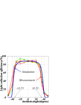
Figure 27: Measured and expected collection efficiency as a function of the incident angle of light. The results with different rotation angles around the PMT axis are shown by four lines; the thick blue line shows their average.

Fig. 28 shows the dependence on incident angle of the light-collection efficiency with the whole camera system.

Figure 28: Incident-angle dependence of the light collection efficiency for the whole camera system. The data points show the measured data and the line shows the expectation from simulations. The absolute efficiency of the measurement was adjusted to that of the simulation at $0^{\circ}$ incident angle.

The relative acceptance was estimated with ADC count summed for all PMTs, and the absolute efficiency was adjusted to that of the simulation at an incident angle of 0^∘. According to this measurement, the angle dependence of the light collection efficiency agrees well with expectations.

4.2.3 Cross-talk effect

The cross-talk effect among the neighboring pixels was investigated by illuminating one PMT module located at the center of the camera with an LED (at about 100 p.e. level). The effect of the cross-talk was investigated while considering the variation of the signals for 47 non-illuminated PMT modules located within a distance of three pixels from the illuminated PMT module. Fig. 29 shows the difference of the ADC count for a non-illuminated PMT module.

Figure 29: Deviation of the ADC count for non-illuminated PMT modules.

The averaged difference for these PMT modules resulted in $-0.37$ count, which corresponds to a cross-talk of less than 0.4%, a negligibly small value.

Two causes of cross-talk can be considered: the location dependence of the PMT module and cross-talk in the signal cables and connectors. For the former, no apparent dependence on location was observed, with the cross-talk being less than 0.08%. For the latter cause a deviation of 0.1% was observed, however, this can also be considered to be negligibly small.

5 Conclusion

The performance of the Cherenkov imaging camera for the second CANGAROO-III telescope was improved over that of the first (CANGAROO-II) telescope with respect to the uniformity of gain, timing resolution and the light-collection efficiency. The 427 camera PMTs and a number of spares have been carefully calibrated and the results stored in a database so that the camera performance can be optimized. The total weight of the camera was measured to be 110 kg. This camera performance matches the expectations from simulations, and is suitable for observations with the next generation of gamma-ray telescopes.

References

- [1] T. Hara, et al., Nucl. Instr. and Meth. A 332 (1993) 300.
- [2] T. Kifune, et al., Astrophys. J. 438 (1995) L91.
- [3] T. Tanimori, et al., Astrophys. J. 492 (1998) L33.
- [4] K. Okumura, et al., 2002, in preparation.
- [5] T. Tanimori, et al., Astrophys. J. 497 (1998) L25.
- [6] H. Muraishi, et al., Aston. Astrophys. 354 (2000) L57.
- [7] R. Enomoto, et al., Nature, 416 (2002) 823.
- [8] M. Mori, et al., in Proc. 27th ICRC (Hamburg, Germany), 5 (2001) 2831.
- [9] H. Kubo, et al., in Proc. 27th ICRC (Hamburg, Germany), 5 (2001) 2900.
- [10] F. Kajino, et al., in Proc. 27th ICRC (Hamburg, Germany), 5 (2001) 2909.
- [11] A. Kawachi, et al., Astropart. Phys., 14 (2001) 261.
- [12] A. Daum, et al., Astropart. Phys. 8 (1997) 1.
- [13] R. Enomoto, et al., Astropart. Phys. 16 (2002) 235.
- [14] C.W. Akerlof, et al., Astrophys. J. 377 (1991) L97.
- [15] Hoffman, W. 1997, in Proc. Towards a Major Atmospheric Cherenkov Detector V, (Kruger Park, South Africa) p.284.
- [16] R.C. Hartman, et al., Astrophys. J. Supp. 123 (1999) 79.
- [17] A.I. Nikishov, Sov. Phys. JETP 14 (1962) 393.
- [18] R.J. Gould, & G. Schrèder, Phys. Rev. 155 (1967) 1408.
- [19] F.W. Stecker, O.C. De Jager, M.H. Salamon, Astrophys. J. 390 (1992) L49.
- [20] H. Hayashida, et al., Astrophys. J. 504 (1998) L71.
- [21] H. Lampeitl, et al., in Proc. Towards a major atmospheric Cherenkov detector (Snowbird 1999) 328-332.
- [22] J.E. Grindlay, et al., Astrophys. J. 201 (1975) 82.
- [23] A.M. Hillas, J. Phys. G: Nucl. Phys. 8 (1982) 1475.
- [24] P.T. Reynolds, et al., Astrophys. J. 404 (1993) 206.
- [25] M.H.R. Khan, Nucl. Instr. and Meth. A 413 (1998) 201.
- [26] K. Tsukada, et al., Nucl. Instr. and Meth. A 300 (1991) 575.
- [27] M. Mori, et al., in Proc. 26th ICRC (Salt Lake City, USA), 5 (1999) 287.
- [28] Hamamatus Photonics K.K., “Photomultiplier Tubes, Basics and Applications (second edition)” p159-160 and Fig. 7-4, Hamamatsu Photonics K.K.
- [29] J.V. Jelly, 1958, “Cherenkov Radiation and its Applications”, Pergamon Press.
- [30] R. Winston, & J. O’Gallagher, Int. Journal of Ambient Energy 4 (1983) 171.
- [31] R. Winston, Scientific American 264 no.3 (1991) 52.