Confirmation of Two Cyclotron Lines in Vela X-1

We present pulse phase-resolved X-ray spectra of the high mass X-ray binary Vela X-1 using the Rossi X-ray Timing Explorer. We observed Vela X-1 in 1998 and 2000 with a total observation time of $\sim$90 ksec. We find an absorption feature at 23.3${}^{+1.3}_{-0.6}$  keV in the main pulse, that we interpret as the fundamental cyclotron resonant scattering feature (CRSF). The feature is deepest in the rise of the main pulse where it has a width of 7.6${}^{+4.4}_{-2.2}$  keV and an optical depth of 0.33${}^{+0.06}_{-0.13}$. This CRSF is also clearly detected in the secondary pulse, but it is far less significant or undetected during the pulse minima. We conclude that the well known CRSF at 50.9${}^{+0.6}_{-0.7}$  keV, which is clearly visible even in phase-averaged spectra, is the first harmonic and not the fundamental. Thus we infer a magnetic field strength of $B=2.6\times 10^{12}$ G.

1 Introduction

Vela X-1 (4U 0900$-$40) is an eclipsing high mass X-ray binary (HMXB) consisting of the B0.5Ib supergiant HD 77581 and a neutron star with an orbital period of 8.964 days (van Kerkwijk et al., 1995) at a distance of $\sim$2.0 kpc (Nagase, 1989). The optical companion has a mass of $\sim$23 $\mbox{M}_{\odot}$ and a radius of $\sim$30 $\mbox{R}_{\odot}$ (van Kerkwijk et al., 1995). Due to the small separation of the binary system (orbital radius: $1.7\,{\rm R_{*}}$), the 1.4 $\mbox{M}_{\odot}$ neutron star (Stickland et al., 1997) is deeply embedded in the intense stellar wind ($4\times 10^{-5}$ $\mbox{M}_{\odot}$ $\text{yr}^{-1}$; Nagase et al., 1986) of HD 77581.

The neutron star has a spin period of $\sim$283 s (Rappaport & McClintock, 1975; McClintock et al., 1976). Both spin period and period derivative have changed erratically since the first measurement as is expected for a wind accreting system. The last measurements with the Burst and Transient Source Experiment (BATSE) resulted in a period of $\sim$283.5 s.

The X-ray luminosity of Vela X-1 is $\sim$$4\times 10^{36}\,{\rm erg\,s}^{-1}$, which is a typical value for an X-ray binary. Several observations have shown that the source is extremely variable with flux reductions to less than 10 % of its normal value (Kreykenbohm et al., 1999; Inoue et al., 1984). In these instances it is not known whether a clump of material in the wind blocks the line of sight or if the accretion itself is choked.

The phase averaged X-ray spectrum of Vela X-1 has been modeled with a power law including an exponential cutoff (White et al., 1983; Tanaka, 1986) or with the Negative Positive EXponential (NPEX-model; Mihara, 1995, see also Eq. 2 below). The spectrum is further modified by strongly varying absorption which depends on the orbital phase of the neutron star (Kreykenbohm et al., 1999; Haberl & White, 1990), an iron fluorescence line at 6.4 keV, and occasionally an iron edge at 7.27 keV (Nagase et al., 1986). A cyclotron resonant scattering feature (CRSF) at $\sim$55 keV was first reported from observations with HEXE (Kendziorra et al., 1992). Makishima et al. (1992) and Choi et al. (1996) reported an absorption feature at $\sim$25 keV to 32 keV from Ginga data. Kreykenbohm et al. (1999) using observations with the Rossi X-ray Timing Explorer (RXTE) and more detailed analysis of older HEXE and Ginga data (Kretschmar et al., 1996; Mihara, 1995) supported the existence of both lines, while Orlandini et al. (1998) reported only one line at $\sim$55 keV based on BeppoSAX observations. Later observations with RXTE also cast some doubt on the existence of the 25 keV line (Kreykenbohm et al., 2000).

CRSFs are due to resonant scattering of electrons in Landau levels in the strong magnetic field ($B\mbox{$\sim$}10^{12}$ G) of neutron stars (see Coburn et al., 2001; Araya & Harding, 1999; Mészáros & Nagel, 1985, and references therein). The energy of the CRSF is given by

$$E_{\rm C}=11.6\text{\,ke\kern-0.89996ptV}\times\frac{1}{1+z}\times\frac{B}{10^{12}\,\text{G}}$$ (1)

$E_{\rm C}$ is the centroid energy of the CRSF in keV, $z$ is the gravitational redshift, and $B$ the magnetic field strength. Therefore, knowing the correct fundamental energy of the CRSF is important for inferring the correct magnetic field strength. This helps in understanding the emission mechanisms of accretion powered X-ray pulsars and the effects of the magnetic field on the X-ray production.

In this paper, Sect. 2 describes the instruments on RXTE, the relevant calibration issues, the software used for the analysis, and the data. Sect. 3 gives an overview of the spectral models used, introduces pulse phase resolved spectroscopy, and discusses the evolution of the spectral parameters over the pulse in 16 phase bins. Later we use fewer bins to increase the significance and discuss the behavior of the 25 keV and 50 keV CRSFs in different pulse phases. In Sect. 4 we discuss the existence of the 25 keV line and review our findings in the context of the other cyclotron sources.

2 Data

2.1 Observations

We observed Vela X-1 with the RXTE in 1998 and again in 2000. The first observation in RXTE-AO3 was made 1998 January 21/22 (JD 2450835.32 – JD 2450836.05) resulting in 30 ksec on-source time. During this observation we encountered an extended low (see Fig. 2); therefore we only used data taken after the extended low, starting about 8 hours after the beginning of the observation at JD 2450835.64 (see Fig. 2). The second observation was in RXTE-AO4 and took place 2000 February 03/04 (JD 2451577.71 – JD 2451579.22) resulting in 60 ksec on-source time. Figs. 2 and 3 show the PCA light-curves of the 1998 and 2000 observations.

2.2 The Instruments: RXTE

RXTE (Bradt et al., 1993) consists of three instruments: the Proportional Counter Array (PCA; Jahoda et al., 1996), the High Energy X-ray Timing Experiment (HEXTE; Rothschild et al., 1998), and the All Sky Monitor (ASM; Levine et al., 1996).

The PCA consists of five co-aligned Xenon proportional counter units (PCUs). It has a total effective area of $\sim$6000 $\text{cm}^{2}$ and a nominal energy range from 2 to 60 keV. Background subtraction in the PCA is done by a model as the instrument is constantly pointed at the source. We used the Sky_VLE-model (see Stark, 1997, for a description), as is appropriate for the count rate of Vela X-1. The response matrix was generated with PCARSP, version 2.43. To account for the uncertainties in the PCA-response matrix, we used systematic errors as given in Table 1. We derived these numbers by fitting a two power law model simultaneously to a PCA and HEXTE spectrum of the Crab nebula and pulsar (see Fig.1). See Wilms et al. (1999) for a discussion of this procedure.

After the analysis was completed and while this paper was in preparation, FTOOLS Patch 5.0.4 was released, introducing PCARSP version 7.10. Tests using the new response matrix, however, show that the best-fit parameters are only marginally different compared to the old matrices, with the only difference being a $\sim$30 % larger value of the hydrogen column and virtually no difference at higher energies.

Table 1: Systematic errors applied to the PCA-data to account for the uncertainties in the 2.43 and 7.10 version of the PCA response matrices. We used the response matrix generated by PCARSP 2.43 to derive the results presented here (see text).

Channels	keV	Syst. (2.43)	Syst. (7.10)
10 – 19	11 – 15	1.0 %	0.3 %
10 – 15	15 – 18	1.0 %	1.3 %
16 – 26	18 – 12	0.5 %	1.3 %
27 – 39	12 – 18	0.5 %	0.3 %
40 – 58	19 – 30	2.0 %	2.0 %

Figure 1: Ratio of PCA and HEXTE data to the best fit model for a Crab observation (obsid 40805-01-05-01, 1999 December 12). The two power laws, which represent the nebula and pulsar, had photon indices $\Gamma_{1}=2.25^{+0.03}_{-0.03}$ and $\Gamma_{2}=1.88^{+0.05}_{-0.03}$ respectively. A single power law model gave $\Gamma=2.13\pm 0.02$, which is in agreement with recent observations by XMM-Newton (Willingale et al., 2001). The PCA response matrix was created with PCARSP 2.43.

Our light-curves and phase-resolved spectra were obtained from binned mode data with a temporal resolution of 250 ms and 128 spectral channels. Due to the gain correction present in these data in the PCA experiment data system, some pulse height analyzer (PHA) channels remain empty. This problem is known and handled properly by PCARSP (Tess Jaffe, priv. comm.). For clarity, these zero counts/sec channels are not shown in our figures. We therefore used the PCA in the energy range from 3.5–21 keV (corresponding to PHA channels 6–45) in our analysis and relied on the HEXTE data above this energy range.

The HEXTE consists of two clusters of four NaI(Tl)/CsI(Na)-Phoswich scintillation detectors each, which are sensitive from 15 keV to 250 keV. The two clusters have a total net detector area of 1600 $\text{cm}^{2}$. See Rothschild et al. (1998) for a detailed description of the instrument. Early in the mission an electronics failure left one detector in the second cluster unusable for spectroscopy. Background subtraction in HEXTE is done by source-background swapping of the two clusters every 32 s throughout the observation (Gruber et al., 1996). HEXTE was used in the standard modes with a time resolution of 8 $\mu$s and 256 spectral channels. The response matrices were generated with HXTRSP, version 3.1. We used HXTDEAD Version 2.0.0 to correct for the dead time. To improve the statistical significance of our data, we added the data of both HEXTE clusters and created an appropriate response matrix by using a 1:0.75 weighting to account for the loss of a detector in the second cluster. This can be safely done as the two cluster responses are very similar. To further improve the statistical significance of the HEXTE data at higher energies, we binned several channels together as given in Table 2. We chose the binning as a compromise between increased statistical significance while retaining a reasonable energy resolution. The binning resulted in statistically significant data from 17 keV up to almost 100 keV (we detect the source at $\sim$75 keV with a 3 $\sigma$ significance in the pulse phase resolved spectra and 5 $\sigma$ in the phase averaged spectra) in the 2000 observation.

Figure 2: RXTE PCA light-curve of the 1998 observation. The variability is not only due to the flaring, but also due to the 283 s pulse. In this and all following light-curves, the count rate has been normalized to one PCU. The temporal resolution of the light-curves is 16 s and covers the entire energy range of the PCA. The gaps in the light-curve are due to Earth occultation and passages through the South Atlantic Anomaly. Note the extended low in the first half of the observation: it is probably due to a massive blob of cold material passing through the line of sight. As this paper is dedicated to phase-resolved spectroscopy and the existence of the CRSFs, this data was excluded from our analysis and we do not discuss this phenomenon here. For a detailed discussion, see Kretschmar et al. (1999). After the extended low, Vela X-1 was flaring and remained so until the end of the observation.

Figure 3: RXTE PCA light-curve of the 2000 observation as for the 1998 observation in Fig. 2. Gaps in the light-curve are due to SAA, Earth occultation, and RXTE observing other sources.

Table 2: Binning of the HEXTE data. We chose the binning to get good statistical significance for each bin while also maintaining good energy resolution. Therefore we did not bin the channels below 40 keV. Factor is the number of channels binned together. Raw channels are approximately 1 keV in width.

Channels	Factor
111 – 139	1
140 – 169	3
170 – 109	8
110 – 255	32

All analysis was done using the FTOOLS version 5.0.1 dated 2000 May 12. We used XSPEC 11.0.1aj, (Arnaud, 1996) with several custom models (see below, Sect. 3.1) for the spectral analysis of the data. To create phase-resolved spectra we modified the FTOOL fasebin, to take the HEXTE dead-time into account. A version of this modified tool is available by contacting the authors.

3 Spectral Analysis

3.1 Spectral Models

Since probably all accretion powered X-ray pulsars have locally super-Eddington flux at the polar cap (Nagase, 1989), a realistic, self-consistent calculation of the emitted spectrum is extremely difficult. Both radiative transfer and radiation hydrodynamics have to be taken into account at the same time (Isenberg et al., 1998). Although this problem has been investigated for many years, there still exists no convincing theoretical model for the continuum of accreting X-ray pulsars (Harding, 1994, and references therein). Most probably, the formation of the overall spectral shape is dominated by resonant Compton scattering (Nagel, 1981b; Mészáros & Nagel, 1985; Brainerd & Mészáros, 1991; Sturner & Dermer, 1994; Alexander et al., 1996). This should produce a roughly power-law continuum with an exponential cutoff at an energy characteristic of the scattering electrons. Deviations should appear at the cyclotron resonant energy, i.e. the cyclotron lines. Because the process is resonant scattering, as opposed to absorption, it is natural to call “cyclotron lines” “cyclotron resonant scattering features”. Because of the computational complexities associated with modeling the continuum and CRSF formation, this type of Comptonization has been far less studied than thermal Comptonization (Sunyaev & Titarchuk, 1980; Hua & Titarchuk, 1995), and empirical models of the continuum continue to be the only option for data analysis.

Due to the general shape of the continuum spectrum, the empirical models all approach a power-law at low energies, and have some kind of cutoff at higher energies (White et al., 1983; Tanaka, 1986). The CRSFs are either modeled as subtractive line features or through multiplying the continuum with a weighting function at the cyclotron resonant energy. As we have shown previously (Kretschmar et al., 1997), a smooth transition between the power law and the exponential cutoff is necessary to avoid artificial, line-like features in the spectral fit. This transition region is notoriously difficult to model. See Kreykenbohm et al. (1999) for a discussion of spectral models with smooth “high energy cutoffs”, such as the Fermi-Dirac cutoff (Tanaka, 1986) used in our analysis of the AO1 data (Kreykenbohm et al., 1999), and the Negative Positive Exponential model (NPEX; Mihara, 1995; Mihara et al., 1998).

In this paper, we describe the continuum of Vela X-1, $I_{\text{cont}}$, using the NPEX model,

$$I_{\text{cont}}(E)\propto\left(E^{-\Gamma_{1}}+\alpha E^{+\Gamma_{2}}\right)\times\text{e}^{-E/E_{\text{F}}}$$ (2)

where $\Gamma_{1}>0$ and $\Gamma_{2}=2$ (Mihara, 1995) and where $E_{\text{F}}$ is the folding energy of the high energy exponential cutoff. In our experience, this model is the most flexible of the different continuum models. For Vela X-1, the continuum between 7 and 15 keV is better described with the NPEX model than the Fermi-Dirac cutoff. The CRSFs are taken into account by a multiplicative factor

$$I(E)\propto I_{\text{cont}}\exp\left(-\tau_{\text{GABS}}(E)\right)$$ (3)

where the optical depth, $\tau_{\text{GABS}}$, has a Gaussian profile (Coburn et al., 2002, Eqs. 6,7),

$$\tau_{\text{GABS}}(E)=\tau_{\text{C}}\times\exp\left(-\frac{1}{2}\left(\frac{E-E_{\text{C}}}{\sigma_{\text{C}}}\right)^{2}\right)$$ (4)

Here $E_{\text{C}}$ is the energy, $\sigma_{\text{C}}$ the width, and $\tau_{\text{C}}$ the optical depth of the CRSF.

We note that the relationship between the parameters of the empirical continuum models and real physical parameters is not known. Because thermal Comptonization spectra get harder with an increasing Compton-$y$-parameter, it seems reasonable to relate the characteristic frequency of the exponential cutoff, $E_{\text{F}}$, with some kind of combination between the (Thomson) optical depth and the temperature (see, e.g., Mihara et al., 1998). Because of the complexity of the continuum and line formation, however, we caution against a literal interpretation of any of the free parameters that enter these continuum models, and will not attempt to present any interpretation here (note, however, that the cyclotron line parameters do have a physical interpretation).

3.2 Pulse Phase-resolved spectra

During the accretion process, material couples to the strong magnetic field of the neutron star at the magnetospheric radius. This material is channeled onto the magnetic poles of the neutron star, where spots on the surface of the neutron star are created (Burnard et al., 1991, and references therein). If the magnetic axis is offset from the spin axis, the rotation of the neutron star gives rise to pulsations (Davidson & Ostriker, 1973), as a distant observer sees the emitting region from a constantly changing viewing angle. Because the emission is highly aniostropic, the spectra observed during different pulse phases vary dramatically. This is especially true for CRSFs whose characteristics depend strongly on the viewing angle with respect to the magnetic field (for an in-depth discussion see Araya-Góchez & Harding, 2000; Araya & Harding, 1999; Isenberg et al., 1998, and references therein). This dependence can in principle be used to infer the geometric properties of the emission region and the electron temperature.

To obtain phase-resolved spectra, the photon or bin times were bary-centered and corrected for the orbital motion of Vela X-1 using the ephemeris of Nagase (1989). Then the pulse phase was calculated for each time bin (for the PCA) or for each photon (for the HEXTE) and then attributed to the appropriate phase bin. Using epoch folding (Leahy et al., 1983), we determined the pulse period for each observation individually. We derived pulse periods of $P_{\text{pulse}}=283.5\pm 0.1$ s for the 1998 data and $P_{\text{pulse}}=283.2\pm 0.1$ s for the 2000 data (using $\text{JD}2444279.546637$ as the zero phase for both observations).

Figure 4: Energy resolved pulse profiles in four bands derived from the 2000 data. At lower energies (below 6 keV), the pulse profile is very complex and shows a five peaked structure: two peaks in the main pulse and three in the secondary pulse. Between 6 keV and 10 keV, the first peak of the main pulse is reduced to a mere shoulder, while the second peak is very strong. Above 10 keV the pulse profile evolves continuously into a simple double pulse.

Since the first detection of pulsations from Vela X-1 by McClintock et al. (1976), the pulse profile is known to be very complex. Above 20 keV, the pulse profile consists of two peaks which are about equally strong. Since Vela X-1 has a relatively hard spectrum, Staubert et al. (1980) were able to detect the two pulses up to 80 keV. We designate these two pulses as the main pulse and the secondary pulse (see Fig. 4 for the definition).

Below 5 kev, these two pulses evolve into five peaks: the main pulse develops into two peaks while the secondary pulse develops into three peaks. Although the two pulses are almost equally strong at high energies, the second peak of the main pulse is almost a factor of two brighter at lower energies than the first two peaks of the secondary pulse, while the third peak of the secondary pulse is almost as strong as the first peak of the main pulse. For a detailed description of the pulse profile and the relative intensities of the different peaks, see Raubenheimer (1990) and Sect. 4.1.

In the following we first study the evolution of the continuum parameters (i.e., the NPEX-model and the photo-electric absorption) and then concentrate on the behavior of the CRSFs in the 2000 and 1998 observations using fewer phase bins.

3.2.1 Spectral Evolution over the Pulse

We used 16 phase bins for the 1998 as well as the 2000 data. The better statistics of the 2000 observation would allow finer resolution (e.g., 32 phase bins) but would make the comparison of the observations more difficult.

The phase resolved spectra were again modeled using the NPEX continuum with $\Gamma_{2}=2$, modified by photoelectric absorption, an iron line at 6.4 keV, and the CRSF at 50 keV. The evolution of the relevant spectral parameters is shown as a function of pulse phase in Figs. 5 and 6 for the 1998 and 2000 data, respectively. Note that in this section, the emphasis is on the evolution of the continuum parameters. The CRSFs will be discussed in detail in the next two sections.

Figure 5: Evolution of the fit parameters over the pulse for the 16 phase-bins for the 1998 data. The spectral hardness is defined as $R=H/S$ where $S$ is the total rate in the 2.5–10 keV band and $H$ is total rate in the 15–20 keV band. The PCA-cts s^-1 PCU^-1 is in the energy range from 15–20 keV and shows clearly the Vela X-1 double pulse. $\alpha$ is the relative normalization of the positive power law of the NPEX-model and $\Gamma_{1}$ is the photon-index of the negative power law of the NPEX-model (see Eq. 2). $E_{\rm C,2}$ is the energy of the CRSF at 50 keV and $\tau_{\rm C,2}$ its depth. The width of the CRSF, $\sigma_{\rm C,2}$, has been fixed at 4 keV. See text for a discussion of the parameters. The vertical bars indicate the uncertainties at 90 % confidence level.

Figure 6: Evolution of the fit parameters over the pulse for the 16 phase-bins for the 2000 data. The spectral hardness, the other parameters, and energy ranges are defined as in Fig. 5. The vertical bars indicate the uncertainties at 90 % confidence level.

The spectral evolution over the pulse of the two observations is somewhat different (see Figs. 5 and 6): in the 1998 data, $N_{\text{H}}$ varies between $15\times 10^{22}\,\text{cm}^{-2}$ and $26\times 10^{22}\,\text{cm}^{-2}$ and shows a clear correlation with flux (linear correlation coefficient $r=0.75$; Bevington & Robinson, 1992, Eq. 11.17). In the 2000 data, $N_{\text{H}}$ is lower by a factor of 10 and consistent with a constant value ($r=0.21$).

In the 1998 data, the folding energy of the NPEX-model is variable with pulse phase: it correlates strongly with flux in the secondary pulse (correlation coefficient $r=0.89$), while there is no such correlation in the main pulse ($r=0.16$). In the 2000 data, this correlation is much less pronounced: $r=0.45$ for the secondary pulse and $r=0.14$ for the main pulse. The photon index $\Gamma_{1}$ of the NPEX model varies over the pulse, but is only correlated with flux in the 1998 data ($r=0.76$). No such correlation is present in the 2000 data ($r=0.21$): its value in most phase bins is consistent with 0.6, which is about a factor of 4 smaller than in the 1998 data. Although the $\chi^{2}$ contours of $N_{\text{H}}$ versus $\Gamma_{1}$ are somewhat elongated, we note that it is impossible to fit the 2000 data with values of $\Gamma_{1}$ and $N_{\text{H}}$ similar to the 1998 data. Such an attempt results in $\chi^{2}>3500$ (66 dof). The relative normalization of the negative power law component of the NPEX model, $\alpha$, varies significantly over the pulse: while there is no clear correlation with flux present in the 1998 data, the 2000 data is clearly correlated with flux ($r=0.75$). The hardness ratio again shows a very strong correlation with flux in the 1998 data ($r=0.95$) and in the 2000 data ($r=0.88$).

Summarizing this section, we found that the two observations are somewhat different. In the 1998 data, the absorption column $N_{\text{H}}$, the photon index $\Gamma_{1}$, the folding energy of the NPEX model, and the hardness ratio are correlated with flux, while all the iron line parameters and the relative normalization $\alpha$ of the NPEX model are not correlated with flux. In the 2000 data, however, the relative normalization of the NPEX model, and the hardness ratio are correlated with flux, while the other parameters are not.

3.2.2 The CRSFs in the 2000 data

Although the 16 phase bins provide good temporal resolution, the relatively low exposure time per bin results in only mediocre statistics. Therefore we reduced the number of phase bins to obtain better statistical quality per bin. For the 2000 data, spectra were obtained for the rise, center, and fall of the main pulse, for the rise, center, and fall of the secondary pulse, and for the two pulse minima (see Fig. 7 for the definition of the individual bins). Henceforth, we identify these phase bins with capital letters.

We used our standard continuum model to analyze the data; since these sections are commited to the CRSFs, we only quote the interesting spectral parameters here (a table of all spectral fits accompanies this paper in electronic form only).

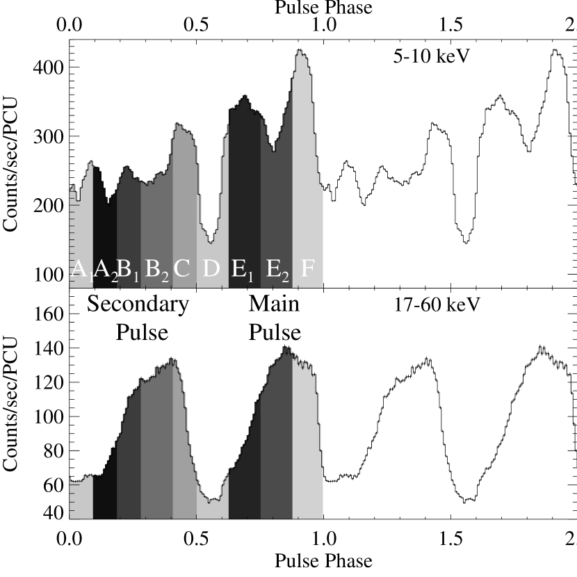
Figure 7: Folded light curves (FLCs) of the 2000 data and definition of the nine phase bins obtained from the 2000 data. As in Fig. 12, we show the complex low energy pulse profile in the upper panel and the simpler high energy pulse profile in the lower panel. Due to the evolution of the pulse period, the FLCs of the 2000 data are somewhat offset compared to the 1998 data FLCs. Note that due to the higher statistics we used nine phase bins in the 2000 data instead of six for the 1998 data. For clarity, the folded light-curve is shown twice. Note that error-bars are shown, but in most cases they are too small to be seen in print.

The well known CRSF at 52.8${}^{+1.9}_{-1.4}$  keV is strongest in the fall of the main pulse with a depth of $\tau_{\rm C,2}=1.1^{+0.3}_{-0.2}$ ($F$-Test: $2.9\times 10^{-14}$). In the center of the main pulse (bin E₂), it is somewhat less deep than in the fall ($\tau_{\rm C,2}=0.5^{+0.3}_{-0.1}$; see Fig. 8). In the rise of the main pulse (bin E₁) it is again of similar depth as in the fall ($\tau_{\rm C,2}=1.0^{+0.4}_{-0.3}$, see Fig. 8).

Figure 8: a Evolution of the depth, the width, and the energy of the CRSF at 23 keV, b evolution of the depth, the width and the energy of the CRSF at 50 keV for the nine phase bins of the 2000 observation. The vertical bars indicate the uncertainties at the 90 % ($2.7\,\sigma$) confidence level. For discussion, see text.

Figure 9: Residuals of fits to the spectrum of the center of the main pulse (bin E₂) of the 2000 data. a for a model without cyclotron absorption lines, b with one line at 53.8${}^{+2.5}_{-1.9}$  keV, and c with two lines at 23.3${}^{+1.3}_{-0.6}$  keV and 54.5${}^{+5.2}_{-2.9}$  keV. Note the feature at 23 keV in b, which we interpret as the fundamental cyclotron absorption line. This line is deepest in the rise and most significant in the center of the main pulse and shallower in the other phase bins (see Fig. 11 and text for discussion).

Figure 10: Residuals of fits to the spectrum of the fall of the main pulse (bin F) of the 2000 data. a for a model without cyclotron absorption lines, b with one line at 52.8${}^{+1.6}_{-1.2}$  keV, and c with two lines at 21.1${}^{+0.6}_{-0.7}$  keV and 52.7${}^{+2.0}_{-1.4}$  keV. The absorption feature at 23 keV in a and b is much weaker than in the center of the main pulse (see Fig. 9), while the 50 keV line is more prominent in this phase bin than in any other phase bin.

Figure 11: Residuals of fits to the fall of the secondary pulse (bin C) of the 2000 data. a for a model without cyclotron absorption lines, b with one absorption line at 50.4${}^{+3.9}_{-2.5}$  keV, and c with two lines at 20.1${}^{+1.4}_{-1.7}$  keV and 50.5${}^{+6.2}_{-3.0}$  keV. The improvement due to the second line at 20 keV is very small; in fact, after the inclusion of the 50 keV line no absorption line feature is visible in b.

In the secondary pulse, the CRSF is on average less deep than in the main pulse and the depth is – within uncertainties – consistent with a constant value of 0.6 throughout the secondary pulse (bins A₁ to C). In the fall (bin C) it has a depth of $\tau_{\rm C,2}=0.5^{+0.2}_{-0.2}$, but it is still very significant ($F$-Test: $1.8\times 10^{-6}$). In the center it is of similar depth ($\tau_{\rm C,2}=0.6^{+0.2}_{-0.2}$) and also very significant ($F$-Test: $3.7\times 10^{-11}$). In the rise (bin B₁) the depth $\tau_{\rm C,2}=0.8^{+0.3}_{-0.2}$ is somewhat greater, but still consistent with a a value of 0.6.

In the pulse minima the significance of the CRSF is low (bin D, $F$-Test: $2.8\times 10^{-2}$) or insignificant (bin A₁; $F$-Test: 0.59). In both cases the depth of the line is $\tau_{\rm C,2}\leq 0.4$ with a lower limit $<0.15$ and an upper limit of $0.5$. Fig. 8 shows the fundamental and harmonic CRSF optical depths in our nine phase bins of the 2000 observation. Given these optical depth measurements and upper limits, we find that in the main pulse, the line is strongest on the rising and falling edges, while it is of similar strength throughout the secondary pulse. Finally, the line is weakest, if indeed present at all, in the pulse minima.

However, after fitting the CRSF at 50 keV, the fit is still not acceptable in most phase bins: there is another absorption line like structure present at about 25 keV. The most straight-forward explanation for this feature is that it is a CRSF. After adding a second CRSF component to our models, the resulting fits are very good. However, as the resulting CRSFs are usually relatively shallow, we also investigated other possibilities to fit this feature, most notably we tried other continuum models like the Fermi-Dirac cutoff. But these models were either completely unable to describe the data (e.g. thermal bremsstrahlung or the cutoffpl, a power-law multiplied by an exponential factor), known to produce artificial absorption lines like the high energy cutoff (White et al., 1983) or – as in the case of the Fermi-Dirac cutoff – also produced an absorption line like feature at 25 keV. The wiggle between $\sim$8 keV and 13 keV, which is present in the 2000 and the 1998 data, is also present in many other RXTE observations of accreting neutron stars (Coburn et al., 2002). It usually has the form of a small dip around 10 keV followed by a small hump at 12 keV (see for instance, Fig. 10); it, however, is very variable. It is present in most phase bins (and in phase averaged spectra), but shows no clear phase dependence. This phenomenon is yet unexplained, but it is unrelated to the feature at 25 keV, since this wiggle appears in many sources at more or less at the same energy where no CRSF is found at 25 keV. We therefore conclude that the feature at 25 keV is real and interpret it as a CRSF.

The behavior of the feature at 25 keV is quite similar to the 50 keV CRSF. We found that the 25 keV line is most significant in the center of the main pulse (bin E₂): the inclusion of a CRSF at 23.3${}^{+1.3}_{-0.6}$  keV improves the fit significantly ($F$-Test: $2.9\times 10^{-13}$). The depth of this line is 0.15, with a lower limit of $0.13$. In the rise of the main pulse (bin E₁), the CRSF at 25.9${}^{+2.4}_{-1.7}$  keV is clearly present and significant ($F$-Test: $2.8\times 10^{-7}$). With a depth of $\tau_{\rm C,1}=0.33^{+0.06}_{-0.13}$ it is also deeper than in the center. However, in the fall (bin F), where the 50 keV line is most prominent, the fundamental line is detected with high significance ($F$-Test: $4.2\times 10^{-9}$), but it is not as deep as in the rise: $\tau_{\rm C,1}=0.13^{+0.05}_{-0.02}$ (see Figs. 8 and 10).

We found that there is also a significant ($F$-Test: $<5\times 10^{-5}$) CRSF present at 23 keV throughout the secondary pulse (B_1,2 and C). As shown in Fig. 8, the line is of similar depth throughout the secondary pulse: from $\tau_{\rm C,1}=0.06^{+0.03}_{-0.02}$ in the fall to $\tau_{\rm C,1}=0.10^{+0.03}_{-0.03}$ in the center, where it is also most significant ($F$-Test: $5.6\times 10^{-10}$). In any case, the line is somewhat shallower than in the main pulse.

In the pulse minimum after the main pulse (bin A₁), an absorption feature at 25 keV is not visible in the residuals and the inclusion of a line at 22.6${}^{+2.9}_{-3.0}$  keV does not result in an improvement ($F$-Test: $0.29$). The upper limit for the depth of this line is 0.10. However, in the pulse minimum before the main pulse (bin D), the residuals show a shallow absorption feature and the inclusion of a CRSF at 20.2${}^{+1.3}_{-1.7}$  keV with a depth of $\tau_{\rm C,1}=0.07\pm 0.03$ improves the fit somewhat ($F$-Test: $3.1\times 10^{-3}$).

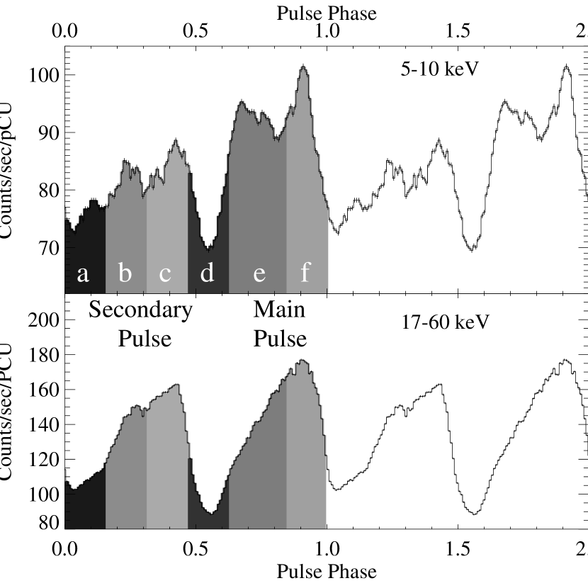
Figure 12: FLCs of the 1998 data. The FLCs were generated by converting the photon arrival times to pulse phases using the spin period of the neutron star and then accumulating a pulse profile binned on phase instead of time. Also shown are the definitions of the pulse phase ranges main pulse fall, main pulse rise, secondary pulse fall, secondary pulse rise, pulse minimum 1, and pulse minimum 2 for the 1998 data for two different energy bands of the PCA (for comparison with the definitions of the 2000 data, see Fig. 7). The upper panel shows the folded low energy pulse profile from 5 to 10 keV, while the lower panel shows the high energy pulse profile above 17 keV. For clarity, the folded light-curve is shown twice. Note that error-bars are shown, but in most cases they are too small to be seen in print.

3.2.3 The CRSFs in the 1998 data

Since the total on-source time of the 1998 data is much less than for the 2000 data, we used only six, broader bins in the 1998 data. We obtained spectra for the rise and fall of the main pulse, the rise and fall of the secondary pulse, and for the two pulse minima (see Fig. 12 for the definition of the individual bins). Henceforth, we identify these phase bins with small letters.

The CRSF at 52.6${}^{+1.4}_{-1.9}$  keV is also most significant in the fall (bin f) of the main pulse ($F$-Test: $8.2\times 10^{-11}$): its depth is 0.8${}^{+0.3}_{-0.2}$. The line is still significant in the rise of the main pulse ($F$-Test: $1.6\times 10^{-4}$; $\tau_{\rm C,2}=0.4^{+0.4}_{-0.1}$). Throughout the secondary pulse (bins b, c), the line has a depth of 0.5${}^{+0.1}_{-0.1}$ similar to the rise of the main pulse and is very significant ($F$-Test: $<1.1\times 10^{-8}$). In the two pulse minima (bins a, d) the CRSF is also present ($\tau_{\rm C,2}=0.4^{+0.1}_{-0.1}$), but less significant than in the rise of the main pulse (bin e; $F$-Test: $<2\times 10^{-3}$). Although the line depth seems to vary over the pulse, it is within errors almost consistent with a constant value of $\tau_{\rm C,2}=0.6$.

After fitting a CRSF at 49.5${}^{+4.0}_{-3.1}$  keV, there is still a feature present at about 25 keV in the spectrum of the main pulse rise (bin e; see Fig. 13) – similar to the 2000 data (see Fig. 9). Fitting another CRSF at 24.1${}^{+1.3}_{-0.7}$  keV with a depth of $\tau_{\rm C,1}=0.08^{+0.03}_{-0.02}$ improves the fit significantly ($F$-test probability for the CRSF being a chance improvement: $6.3\times 10^{-5}$).

In the fall of the main pulse there is also an indication of the presence of an absorption feature at 25 keV after fitting the 52.7${}^{+1.6}_{-1.1}$  keV CRSF. Fitting another cyclotron absorption line at 23.6${}^{+1.0}_{-2.2}$  keV with a depth of $\tau_{\rm C,1}=0.06^{+0.01}_{-0.02}$ improves the fit with an $F$-test probability of $2.7\times 10^{-3}$.

However, between the two pulses we found no significant line at 24 keV: in the pulse minimum 1 (bin a) and pulse minimum 2 (bin d), the inclusion of a CRSF at 23.9${}^{+2.1}_{-1.9}$  keV resulted in no significant improvement; upper limits for the depth of the line are 0.06 (pulse minimum 1) and 0.05 (pulse minimum 2). The same applies for the spectra of the rise and fall of the secondary pulse (bins b and c): the inclusion of a CRSF at 24 keV does not improve the fit significantly ($F$-Test: $>9.8\times 10^{-2}$). Note that this does not exclude the presence of a CRSF at 24 keV, it is just not detected: the upper limit for the depth of the CRSF at 24 keV is $0.04$ for these phase bins.

Figure 13: Residuals of fits to the spectrum of the rise of the main pulse of the 1998 data (bin e). a for a model without cyclotron absorption lines, b with one line at 53.0${}^{+1.8}_{-1.4}$  keV, and c with two lines at 25.1${}^{+1.9}_{-1.3}$  keV and 53.0${}^{+3.8}_{-1.9}$  keV. Note the absorption feature at 25 keV in b which is not present or much weaker in the other pulse phases.

Table 3: Fit results for some selected phase bins from the 2000 data. All uncertainties quoted in this paper are at the 90 % ($2.7\,\sigma$) confidence level. Note that there is an improvement when using a line at 25 keV also in the secondary pulse but this improvement is very small compared to the improvement in the center of the main pulse (see below). The complete tables for the 1998 and 2000 data are available in electronic form only.

	Main Pulse Fall (F)			Secondary Pulse Fall (C)			Main Pulse Center (E2)
	w/o cycl.	1 cycl.	2 cycl.	w/o cycl.	1 cycl.	2 cycl.	w/o cycl.	1 cycl.	2 cycl.
$N_{\text{H}}$ $[10^{22}]$	2.4${}^{+0.5}_{-0.8}$	2.5${}^{+0.4}_{-1.8}$	2.4${}^{+0.9}_{-0.6}$	4.2${}^{+0.5}_{-0.9}$	4.2${}^{+0.2}_{-1.3}$	4.2${}^{+0.6}_{-0.8}$	1.9${}^{+0.5}_{-0.9}$	1.8${}^{+0.3}_{-1.3}$	2.9${}^{+0.4}_{-1.2}$
$\Gamma_{1}$	0.72${}^{+0.04}_{-0.07}$	0.61${}^{+0.06}_{-0.06}$	0.81${}^{+0.12}_{-0.08}$	1.04${}^{+0.04}_{-0.08}$	0.98${}^{+0.06}_{-0.07}$	1.07${}^{+0.06}_{-0.08}$	0.36${}^{+0.06}_{-0.07}$	0.29${}^{+0.07}_{-0.07}$	0.58${}^{+0.10}_{-0.11}$
$\Gamma_{2}$	$2$	$2$	$2$	$2$	$2$	$2$	$2$	$2$	$2$
$E_{\text{F}}$	6.36${}^{+0.03}_{-0.03}$	6.38${}^{+0.09}_{-0.06}$	6.37${}^{+0.08}_{-0.07}$	5.95${}^{+0.04}_{-0.03}$	6.14${}^{+0.09}_{-0.06}$	6.04${}^{+0.08}_{-0.07}$	6.14${}^{+0.03}_{-0.03}$	6.28${}^{+0.04}_{-0.04}$	6.02${}^{+0.17}_{-0.05}$
$E_{\rm C,1}$ [keV]	–	–	21.1${}^{+0.7}_{-0.7}$	–	–	20.1${}^{+1.3}_{-1.6}$	–	–	23.3${}^{+1.3}_{-0.6}$
$\sigma_{\rm C,1}$ [keV]	–	–	4.1${}^{+1.6}_{-0.7}$	–	–	2.8${}^{+1.4}_{-0.9}$	–	–	4.9${}^{+1.9}_{-0.8}$
$\tau_{\rm C,1}$	–	–	0.13${}^{+0.05}_{-0.02}$	–	–	0.06${}^{+0.03}_{-0.02}$	–	–	0.15${}^{+0.07}_{-0.02}$
$E_{\rm C,2}$ [keV]	–	53.0${}^{+1.6}_{-1.2}$	52.8${}^{+1.9}_{-1.4}$	–	50.5${}^{+3.9}_{-2.4}$	50.6${}^{+4.9}_{-2.7}$	–	53.8${}^{+2.3}_{-1.9}$	54.5${}^{+5.0}_{-2.8}$
$\sigma_{\rm C,2}$ [keV]	–	4.9${}^{+1.2}_{-0.9}$	4.7${}^{+1.5}_{-1.2}$	–	4.9${}^{+2.6}_{-2.5}$	5.4${}^{+3.4}_{-2.4}$	–	3.7${}^{+1.6}_{-1.6}$	5.3${}^{+5.1}_{-2.8}$
$\tau_{\rm C,2}$	–	1.3${}^{+0.3}_{-0.2}$	1.1${}^{+0.3}_{-0.2}$	–	0.6${}^{+0.4}_{-0.2}$	0.5${}^{+0.2}_{-0.2}$	–	0.8${}^{+0.5}_{-0.2}$	0.5${}^{+0.3}_{-0.1}$
$\chi^{2}(\text{dof})$	424 (64)	144 (61)	62 (58)	121 (64)	75 (61)	50 (58)	258 (64)	174 (61)	61 (58)

4 Summary and Discussion

4.1 The Pulse Profile

Despite the strong pulse to pulse variations and the overall strong variability of Vela X-1 including flaring activity (see Fig. 2, 3) and “off-states” (Kreykenbohm et al., 1999; Inoue et al., 1984), the pulse profile at higher and lower energies is remarkably stable (compare the pulse profile in Fig. 4 and e.g. McClintock et al., 1976). Therefore, the low energy profile is not due to any random short term fluctuations.

Such an evolution of the pulse profile and therefore the spectral shape over the X-ray pulse is typical for accreting X-ray pulsars, however, its interpretation is difficult. While the double pulse at energies above 20 keV can be attributed to the two magnetic poles (Raubenheimer, 1990), there is no such straightforward explanation for the low energy pulse profile.

Early explanations of the pulse profile invoked varying photoelectric absorption over the pulse (Nagase et al., 1983). In this picture, for example, the “dip” at pulse phase $\sim$0.8 is attributed to the accretion column passing through the line of sight. However, there is no such straightforward explanation for the complex profile of the secondary pulse and furthermore, our phase resolved spectra do not show an increased absorption in the center of the main pulse (Fig. 6). It therefore seems more plausible to attribute the variation of the spectral parameters with pulse phase to the mechanism generating the observed radiation, such as anisotropic propagation of X-rays in the magnetized plasma of the accretion column (Nagel, 1981a) or the influence of the magnetic field configuration (Mytrophanov & Tsygan, 1978). Due to the uncertainties associated with modeling the accretion column (see Sect. 3.1), only the general shape of the pulse profile can be described with these models, and the substructures cannot be explained. A good description of the processes responsible for the complex shape of the pulse profile is thus still missing.

We note, however, that in the strong magnetic field of the accretion column the motion of electrons perpendicular to the magnetic field is constrained, while they move freely parallel to the field lines. As a result, one expects the thermal motion of the electrons to produce a harder spectrum when viewed parallel to the $B$-field than when viewed perpendicular to the field. In a pencil beam geometry, one would then expect the pulse maxima to have a harder spectrum than the minima, similar to what has been seen in Vela X-1.

4.2 The existence of the 25 keV line

It is very unlikely that the 25 keV feature results from a calibration problem. Fits to Crab spectra taken close to the 2000 observation have shown that there are no deviations in the relevant area between 20 keV and 30 keV in the HEXTE (see Fig. 1). Furthermore, we have limited the energy range of the PCA to $\leq$21 keV, so the detection of the line is almost only due to the HEXTE. Finally, we note that the line is only visible in one pulse phase of the 1998 data, which should be subject to similar calibration uncertainties as the 2000 data. Since the HEXTE has a continuous automatic gain control, the HEXTE response is very stable throughout the mission, and thus the calibration is the same for AO1 through AO4.

Our observations indicate that the feature is quite variable with pulse phase. As discussed in the previous sections, the depth of the line varies strongly with pulse phase. In certain phase bins, the lower limit of the depth is 0.20, while in another phase bin its upper limit is 0.09. This variability also makes it highly unlikely that the 25 keV feature is due to a calibration problem as it would then be present in all phase bins. Apart from that, the feature appears at about half the energy of the 50 keV cyclotron line: the lower line is at 22.9${}^{+2.9}_{-0.9}$  keV, while the second line is at 50.9${}^{+0.6}_{-0.7}$  keV (2000 data, phase-averaged spectrum). This results in an average coupling factor of $2.15\pm 0.19$, in agreement with a factor of 2.0 expected for a first harmonic. We also note that in the main pulse rise (2000 data) where the 25 keV CRSF is deepest, we find a coupling factor of almost exactly 2.0. However, we caution that although theoretical models predict a value of 2.0 (Harding & Daugherty, 1991, and references therein), recent observations have shown that the fundamental line can be heavily distorted (as in 4U 0115+63; Heindl et al., 1999; Santangelo et al., 1999) and therefore a coupling factor of exactly 2.0 is not necessarily to be expected.

Furthermore, the 25 keV line varies with time: It was barely visible in the 1998 data and was not seen at all by BeppoSAX (Orlandini et al., 1998). Adding to that, the strong phase variability of the line makes it difficult to detect. Therefore it is not surprising that Orlandini et al. (1998) and Kreykenbohm et al. (2000) did not detect this line in their phase-averaged spectra. Using phase resolved Ginga data, Mihara (1995) also reported a feature at 24 keV in the main pulse while it was insignificant outside the main pulse.

Figure 14: Raw HEXTE count rate spectrum of the center of the main pulse divided by the raw HEXTE count rate spectrum of the fall of the secondary pulse using the 2000 data. Note the clear lack of counts between 20 keV and 30 keV in the spectrum of the center of the main pulse.

Finally, to be completely independent of any applied model or response matrices, we divided the raw count rate spectrum of the center of the main pulse by the count rate spectrum of the fall of the secondary pulse. The result is shown in Fig. 14: there is a clear dearth of counts between 20 keV and 30 keV, just where we find the 25 keV line with about the same width. This means that there is an absorption line like feature in the raw count rate spectrum of the center of the main pulse – independent of the applied model or the response matrix.

In summary, we have shown that there is an absorption line like feature at 25 keV in some phase bins, while it is shallower or far less significant in other phase bins. The most straightforward interpretation of this feature is that it is the fundamental CRSF, while the 50 keV line is the first harmonic.

4.3 CRSFs in accreting pulsars

Figure 15: Correlation between the centroid energy of the fundamental CRSF and the cutoff energy (when using a power law/high energy cutoff model instead the NPEX model), based on RXTE data (with the exception of A 0535$+$26). See Coburn (2001) for a complete discussion. With a line energy of 25 keV, Vela X-1 fits nicely into the sequence, whereas it would not fit in if the energy of the fundamental line were 50 keV.

There are now about a dozen X-ray pulsars for which cyclotron lines have been detected. Most of these sources have been observed with RXTE, such that a systematic study of the properties of these sources and their CRSFs starts to become feasible. Although such a study is outside the scope of this paper, we want to point out that our detection of a CRSF at $\sim$25 keV in Vela X-1 is consistent with the general properties of CRSF sources. In their study of CRSFs from Ginga and other instruments, Makishima et al. (1999) found a correlation between the energy of the fundamental CRSF and the cutoff energy in the canonical White et al. (1983) X-ray pulsar continuum. Recently, this correlation has been reinvestigated by Coburn (2001) using RXTE data from all sources with known CRSFs. Since RXTE has a broader energy range than previous missions, such a study is able to cover a wider range of CRSF energies. Coburn (2001) finds that most RXTE observed pulsars follow the Makishima et al. (1999) correlation up to 35 keV where a roll-over is observed (see Fig. 15 and Coburn, 2001, for a discussion).

The only exceptions so far are GX 301$-$2 which shows very high amplitude $N_{\text{H}}$ variations which make the determination of the continuum uncertain, 4U 1626$-$67 follows the correlation only in certain pulse phases, while X Per has a very different continuum (Coburn et al., 2001) and therefore a comparison with the other sources is difficult if possible at all.

We note that Vela X-1 fits nicely the correlation of Fig. 15, provided the fundamental line is at $\sim$25 keV and not at 50 keV.

As we have pointed out in section 4.2, the fundamental line in Vela X-1 is weak and only detectable in some specific pulse phases. This is similar to the other three sources where more than one fundamental CRSF has been claimed so far: 4U 0115$+$63 (Heindl et al., 1999; Santangelo et al., 1999), A 0535$+$26 (Kendziorra et al., 1994; Maisack et al., 1997), and 4U 1907$+$07 (Cusumano et al., 1998). In 4U 0115$+$63, the fundamental CRSF is quite complex and decidedly non-Gaussian in shape – Heindl et al. (1999) require two overlapping lines in order to model this line, while the higher 4 harmonics are much more Gaussian in shape. Here, all lines show strong variation with pulse phase, but are almost always present. For A 0535$+$26, a very prominent line at $\sim$100 keV has been reported by Maisack et al. (1997) using OSSE, while a 50 keV feature presented by Kendziorra et al. (1994) from HEXE data was quite weak and difficult to model. Finally, Cusumano et al. (1998) find in 4U 1907$+$09, that the line at 39 keV is again very prominent while its $\sim$19 keV fundamental is weak.

Such a complex line shape of the fundamental line is consistent with Monte Carlo simulations of the generation of cyclotron lines in accreting X-ray pulsars (Isenberg et al., 1998; Araya & Harding, 1999; Araya-Góchez & Harding, 2000). These simulations show that the shape of the CRSF depends strongly on the assumed geometry, electron temperature, and optical depth of the plasma. It has been pointed out by Araya & Harding (1999), that under certain viewing angles, the fundamental line is not a simple absorption line, but has a very complex shape that includes, for example, “P Cygni” like emission wings. These emission wings are caused by the angular dependence of the scattering cross section, multiple resonant scattering, and by higher order effects such as “photon spawning” (Araya-Góchez & Harding, 2000).

The feature seen around 20 keV (Figs. 9, 10, and 11) might be such an emission wing. Fitting this feature (where present) with a Gaussian produces a fit comparable to fitting an absorption line. The resulting Gaussians are relatively narrow: 0.7${}^{+0.6}_{-0.7}$  keV in the fall of the secondary pulse and 1.5${}^{+0.2}_{-0.4}$  keV in the fall of the main pulse. The Gaussian is broadest in the rise of the main pulse with a width of 3.0${}^{+1.0}_{-0.7}$  keV. Due to this narrowness we believe that this feature is a wing of a CRSF and not due to improper modeling of the continuum, e.g. due to a Wien bump between 10 keV and 20 keV which would have to be much broader.

Higher order CRSFs tend to be much less affected by these phenomena. When such complicated line profiles are convolved with the moderate energy resolution of todays X-ray detectors, it is possible that such emission wings result in line profiles where the line is almost undetectable or where the line shows the shallow non-Gaussian shape seen in 4U 0115$+$63. Since the strength of the wings depends on the inclination angle, one could envisage a scenario where the geometry of the accretion column is such that the fundamental is completely filled in except for certain pulse phases, explaining the difficulty of detecting the fundamental CRSF in these systems. Admittedly, these simulations have only begun and the computation of larger grids of simulated and more realistic CRSFs for observational work has only recently become computationally feasible. However, if this speculation were true, it would provide a natural explanation for the scarcity of X-ray pulsars where more than one CRSF is observable.