A Fast Algorithm for Solving the Poisson Equation on a Nested Grid

Abstract

We present a numerical method for solving the Poisson equation on a nested grid. The nested grid consists of uniform grids having different grid spacing and is designed to cover the space closer to the center with a finer grid. Thus our numerical method is suitable for computing the gravity of a centrally condensed object. It consists of two parts: the difference scheme for the Poisson equation on the nested grid and the multi-grid iteration algorithm. It has three advantages: accuracy, fast convergence, and scalability. First it computes the gravitational potential of a close binary accurately up to the quadraple moment, even when the binary is resolved only in the fine grids. Second residual decreases by a factor of 300 or more by each iteration. We confirmed experimentally that the iteration converges always to the exact solution of the difference equation. Third the computation load of the iteration is proportional to the total number of the cells in the nested grid. Thus our method gives a good solution at the minimum expense when the nested grid is large. The difference scheme is applicable also to the adaptive mesh refinement in which cells of different sizes are used to cover a domain of computation.

1 Introduction

Astronomical objects such as stars, clouds, and galaxies have enormous dynamic range both in density and in size. To illustrate this enormous dynamic range, we consider star formation as an example. Stars form in molecular clouds of which the mean density is 10³ atoms cm^-3. The molecular clouds contain condensations named molecular cloud cores, from which stars form owing to the self-gravity. The molecular cloud cores have typical size of 10¹⁷ cm and typical density of 10⁵ atoms cm^-3. On the other hand, the central density of a star is 10¹¹ atoms cm^-3 at the very beginning of its protostellar stage and the present Sun has the central density of 10²⁶ atoms cm^-3. The radius of a protostar is 10¹⁴ cm when the central density is 10¹² atoms cm^-3. As the central density increases, the radius decreases down to 10¹⁰ – 10¹² cm until the star reaches its main sequence (hydrogen burning) stage.

This enormous dynamic range restrict us to achieve high spatial resolution only in the small regions of interest. To generate finer grids in the region of interest, people have developed various mesh generation methods. Adaptive mesh refinement (AMR) and nested grids (NG) are typical of the mesh generation methods developed in the past decade. AMR and NG generate finer grids hierarchically in the region of interest. AMR was invented by Berger & Oliger (1984) and has been advanced by many researchers. NG is a variant of AMR and generates only one sub-grid at each hierarchical level, while AMR has no restriction on the number of sub-grids. AMR and NG have succeeded in simulations of star formation and galaxy formation in which compact objects form by condensation of diffuse clouds.

Some recent numerical simulations on star formation and cosmology apply either AMR or NG to achieve high spatial resolution. Truelove et al. (1997) studied gravitational collapse of a molecular cloud core with AMR to resolve fragmentation of the highly condensed cloud core. Since then AMR is frequently used in numerical simulations of fragmentation during gravitational collapse (Truelove et al., 1998; Boss et al., 2000). Using NG Burkert & Bodenheimer (1993, 1996) studied fragmentation of a centrally condensed protostar. They succeeded in resolving spiral arms formed by the self-gravitational instability in the protoplanetary disk. Using NG Tomisaka (1998) computed gravitational collapse of rotating magnetized gas cloud and found magnetohydrodynamical driven outflow emanating from a very compact central disk. Norman & Bryan (1999) has reviewed application of AMR to cosmological simulations.

Though simulations based on AMR and NG are successful, some technical problems still remain for AMR and NG. One of them is a numerical algorithm for solving the Poisson equation on a grid in which a cell faces several smaller cells. In other words, difficulty arises at boundaries between the regions covered with different size cells. For later convenience we name these boundaries the grid level boundaries. In most AMR and NG of three dimensions, a parent cell faces four child cells at each grid level boundary in case of three dimensions.

When cells are uniform on a grid, a simple central difference scheme gives us second order accuracy and the difference equation can be solved fast with the multi-grid iteration or some other methods. Since the simple central difference breaks down at the grid level boundary, we need some modifications at the boundaries. An ideal scheme should provide an accurate solution and require minimum computation load. As shown later, some schemes published in recent literature lack in accuracy.

One might think that we could obtain a good solution by relatively small computation cost if we would solve the Poisson equation successively from coarse grids to fine grids. One can solve the Poisson equation on the coarsest grid if an appropriate boundary is given at the boundary of the grid. Then the solution gives boundary conditions for the sub-grid if we interpolate it appropriately. Thus we can solve the Poisson equation on the sub-grid and repeat the same procedure down to the finest grid. This algorithm requires rather small computation load but the solution is not accurate enough.

To illustrate the problem of the algorithm mentioned above, we consider binary or multiple stars of which separation is too short to resolve in a coarse grid. For simplicity we assume that the binary or multiple stars dominate the gravity. At a large distance from them, the gravity is approximately the sum of the point mass gravity and the quadraple moment of gravity. If we compute the gravity with a coarse grid without any knowledge on the fine structure, we will miss the quadraple moment of gravity. Although it is smaller than the point mass gravity, the quadraple moment of gravity is the leading term in the gravitational torque. We need to take account of mass distribution in a fine grid to evaluate the gravitational torque.

In this paper we present a difference equation for the Poisson equation on a nested grid. The solution of this difference equation is accurate enough in the sense that it reproduces the quadraple moment of gravity quantitatively even in a coarse grid. Moreover the difference equation can be solved fast with the multi-grid iteration. The computation load is scalable, i.e., proportional to the total number of cells involved in the nested grid.

The above difference equation is also applicable to AMR. The difference equation is likely to be solved fast also with a multi-grid iteration.

In §2 we describe our difference equation. In §3 we denote our algorithm for solving the difference equation. In §4 we show the performance of our scheme with emphasis on the accuracy of the solution and speed of computation. In §5 we discuss reason for success of our difference equation in reproducing the quadraple moment of gravity. We also discuss extension of our method to AMR.

2 Difference Equation

First we introduce our nested grid and define the coordinates. The nested grid consists of uniform grids each of which has cubic cells. The center of each cell is located at

$$x_{i}^{(\ell)} = 2^{-\ell+1}\,(i\,+\,1/2)\,h\,,$$ (1)

$$y_{j}^{(\ell)} = 2^{-\ell+1}\,(j\,+\,1/2)\,h\,,$$ (2)

$$z_{k}^{(\ell)} = 2^{-\ell+1}\,(k\,+\,1/2)\,h\,,$$ (3)

where $i$, $j$, $k$ and $\ell$ are integer and labels. The symbol, $h$, denotes the grid spacing in the coarsest grid at the level of $\ell\,=\,1$. As $\ell$ increases by one, the grid spacing reduces to half. We define the range of $i$, $j$, $k$, and $\ell$ as

$$-N/2\;\leq i \leq\;N/2\,-\,1\;,$$ (4)

$$-N/2\;\leq j \leq\;N/2\,-\,1\;,$$ (5)

$$-N/2\;\leq k \leq\;N/2\;-\,1,$$ (6)

$$1\;\leq \ell \leq\;\ell_{\rm max}\;,$$ (7)

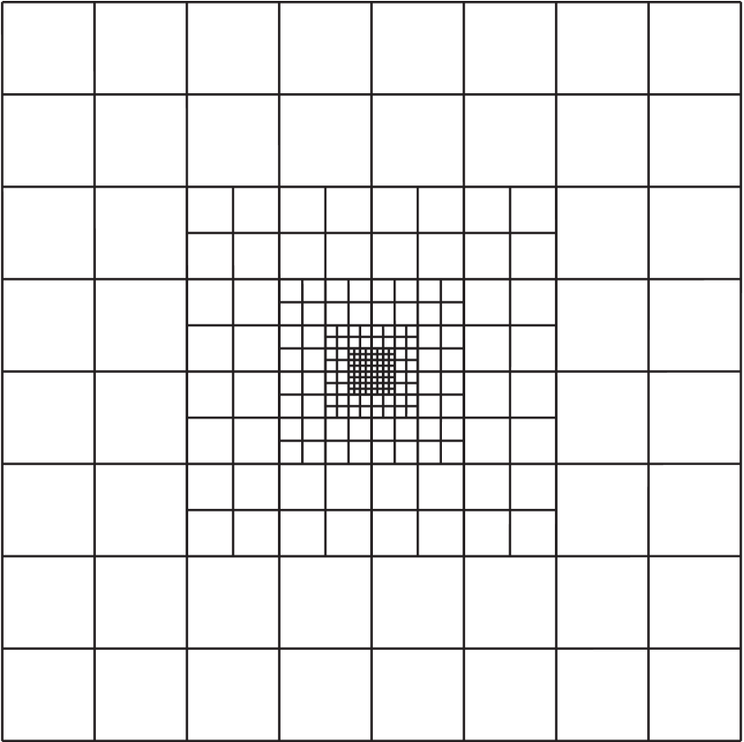
Figure 1: The cross section of our nested grid is shown. The lines denote the cell boundaries. The region closer to the center is covered with a smaller cells. This nested grid has the parameters, $N$ = 8 and $\ell_{\rm max}$ = 5.

in this paper. Thus our nested grid has $\ell_{\rm max}\,\times\,N^{3}$ cells in total. To use the multi-grid iteration effectively, we take $N\,=\,2^{n}$ in our computation. The coarsest grid covers the volume of $L^{3}$, where $L\,=\,N\,h$. The finest grid has grid spacing of $2^{\ell_{\rm max}\,-\,1}\,h$. Since all these grids are concentric, central regions are covered multiply with these grids. When a volume is covered with different size cells, we adopt a quantity in the smallest cell in the final solution. Figure 1 illustrates cell distribution in our nested grid. It denotes the cross section in the two dimension for simplicity.

The gravitational potential is evaluated at the cell center and is labeled as

$$\phi_{i,j,k}^{(\ell)}\;=\;\phi\,[x_{i}^{(\ell)},\,y_{j}^{(\ell)},\,z_{k}^{(\ell)}]\;.$$ (9)

Also the cell averaged density is labeled as

$$\rho_{i,j,k}^{(\ell)}\;=\;\rho\,[x_{i}^{(\ell)},\,y_{j}^{(\ell)},\,z_{k}^{(\ell)}]\;.$$ (10)

The Poisson equation,

$$4\pi G\rho\;=\;\mbox{\boldmath$\nabla$}\cdot\mbox{\boldmath$g$}\;,$$ (11)

and

$$\mbox{\boldmath$g$}\;=\;\mbox{\boldmath$\nabla$}\phi\;,$$ (12)

relates the gravitational potential and density, where $g$ denotes the gravity. When a cell is surrounded by cells of the same size, we obtain the discrete Poisson equation of the second order accuracy,

$$4\pi G\rho_{i,j,k}^{(\ell)} = \frac{g_{x,i+1/2,j,k}^{(\ell)}\,-\,g_{x,i-1/2,j,k}^{(\ell)}}{2^{-\ell+1}h}\;+\;\frac{g_{y,i,j+1/2,k}^{(\ell)}\,-\,g_{y,i,j-1/2,k}^{(\ell)}}{2^{-\ell+1}h}$$ (13)

$$\;+\;\frac{g_{z,i,j,k+1/2}^{(\ell)}\,-\,g_{z,i,j,k-1/2}^{(\ell)}}{2^{-\ell+1}h}\;,$$

and

$$g_{x,i+1/2,j,k}^{(\ell)} = \frac{\phi_{i+1,j,k}^{(\ell)}\,-\,\phi_{i,j,k}^{(\ell)}}{2^{-\ell+1}h}\;,$$ (14)

$$g_{y,i,j+1/2,k}^{(\ell)} = \frac{\phi_{i,j+1,k}^{(\ell)}\,-\,\phi_{i,j,k}^{(\ell)}}{2^{-\ell+1}h}\;,$$ (15)

$$g_{z,i,j,k+1/2}^{(\ell)} = \frac{\phi_{i,j,k+1}^{(\ell)}\,-\,\phi_{i,j,k}^{(\ell)}}{2^{-\ell+1}h}\;,$$ (16)

by the central difference as in case of the uniform grid. Note that the gravity is evaluated on the cell surface.

Equations (14) through (16) need to be modified near the grid boundary. We set the condition that the gravity evaluated in the coarse grid is equal to the average gravity on the smaller cell surfaces, e.g.,

$$g_{x,i+1/2,j,k}^{(\ell)} = \frac{1}{4}\,[g_{x,2i+3/2,2j,2k}^{(\ell+1)}\,+\,g_{x,2i+3/2,2j,2k+1}^{(\ell+1)}$$ (17)

$$\,+\,g_{x,2i+3/2,2j+1,2k}^{(\ell+1)}\,\,+\,g_{x,2i+3/2,2j+1,2k+1}^{(\ell+1)}]\;.$$

This ensures that our solution satisfies the Gauss’s theorem. When we sum up the normal component of the gravity over the surface of a given volume, it equals to the mass contained in the volume multiplied by $4\pi G$.

$$\sum_{\rm surface}\mbox{\boldmath$g$}\cdot d\mbox{\boldmath$S$}\;=\;4\pi G\,\sum_{\rm volume}\rho\,dV\;.$$ (18)

In other words, the “gravitational field line” never ends at the grid level boundary. This is also equivalent to set the Neumann condition at the grid level boundary.

When the cell surface is on the grid level boundary, we interpolate $\phi$ in the coarse grid to evaluate the gravity across the cell surface. As an example we show the interpolation formula to compute the gravity in the $x$-direction in the following. When $i\,=\,N/2\,-\,1$, we evaluate

$$g_{x,i+1/2,j,k}^{(\ell)}\,=\,\frac{\phi_{i+3/2,j,k}^{*(\ell)}\,-\,\phi_{i,j,k}^{(\ell)}}{(3/2)\times 2^{-\ell+1}h}\;,$$ (19)

where $\phi_{i+3/2,j,k}^{*(\ell)}$ denotes the gravitational potential at $(x,\,y,\,z)$ = $[x_{i+3/2}^{(\ell)}\,\equiv\,x_{(i+1)/2}^{(\ell-1)},\,y_{j}^{(\ell)},\,z_{k}^{(\ell)}]$. It is obtained by the interpolation on the diagonal in the coarse cell surface. When $j$ and $k$ are odd numbers, it is evaluated to be

$$\phi_{i+3/2,j,k}^{*(\ell)}\;=\;\frac{3}{4}\,\phi_{(i+1)/2,(j-1)/2,(k-1)/2}^{(\ell-1)}\;+\;\frac{1}{4}\,\phi_{(i+1)/2,(j+1)/2,(k+1)/2}^{(\ell-1)}\;.$$ (20)

Equation (20) uses the gravitational potential at the both ends of the diagonal for the linear interpolation. This interpolation is not unique; we can use the bi-linear interpolation in the coarse cell surface. The result depends little on the interpolation adopted. The cell number at the both ends of the diagonal depends on the even-odd parity of $j$ and $k$. Equation (20) should be modified appropriately when either $j$ or $k$ are even.

Equations (14)-(16) are central difference, our difference equations are the second order accurate except across the grid level boundaries. Since equations (19) and (20) are the first order accurate, our difference equations are only the first order accurate across the boundaries.

We need the gravity at the cell center in the hydrodynamical computation. The gravity at the cell center is evaluated to be the average of those at the opposing cell surfaces, e.g.,

$$g_{x,i,j,k}^{(\ell)}\;=\;\frac{1}{2}\,\left[g^{(\ell)}_{x,i+1/2,j,k}\,+\,g^{(\ell)}_{x,i-1/2,j,k}\right]\;.$$ (21)

We examine the accuracy of the gravity at the cell center in §4.

3 Iterative Method for Solving Difference Equation

Our difference equation can be solved with a simple point Jacobi iteration or red-black Gauss-Seidel iteration but with too many times iteration of the order of $N^{2}$. Thus we adopt the multi-grid iteration for to accelerate the convergence. We employ the Full Multi-Grid (FMG) scheme, i.e., the algorithm shown in Press & Teukolsky (1991) in our paper. Our numerical procedures are rather complicated partly because the FMG scheme is complicated and partly because our nested grid is complex. Thus, we first outline our scheme in the following. Detailed numerical procedures are shown later.

Essence of the multi-grid iteration is to obtain a better initial guess for finer grids from an approximate solutions on coarser grids (see, e.g., Wesseling, 1992; Briggs, Henson, & McCormick, 2000, for the basic of multi-grid iteration). When grids are coarse, the computation cost is less. When interpolated for a fine grid, the solution on a coarse grid is a good initial guess and a better solution on the fine grid is obtained by only a few times iterations.

As a coarse grid, we use another nested grid which covers the same computation volume with a fewer $N$ and larger $h$. More specifically we use the nested grids of $(N,\,h)$ = $(2^{n-1},\,2h_{0})$, $(2^{n-2},\,2^{2}h_{0})$, …., and $(2^{2},\,2^{n-2}h_{0})$, as temporarily working nested grids for computation on the nested grid of $(N,\,h)$ = $(2^{n},\,h_{0})$ (see Chapter 9 of Briggs, Henson, & McCormick, 2000, for the reasoning on our choice of coarsening). Furthermore, we introduce two uniform grids one of which has $2^{3}$ cells and the other of which has only 1 cell. Both the uniform grids covers the whole computation domain which is covered only with the largest grid in the nested grid. Introduction of these temporarily working grids increases the total number of cells in our computation only a factor of 8/7. Accordingly the computation on these working nested grids is only a minor fraction.

We start from an exact solution on the uniform grid having only one cell. The solution is used as an initial value to obtain the solution on the other uniform grid. The obtained solution is used to obtain the solution on the nested grid of $(N,\,h)$ = $(2^{2},\,2^{n-2}h_{0})$. This solution is obtained by the Successive Over Relaxation (SOR, see, e.g. Press et al., 1986, for the basic of SOR). The computation cost is very small since this nested grid contains only $64\,\ell_{\rm max}$ cells. We obtained a solution on the coarsest grid after $4\ell_{\rm max}$ times iteration in a typical model. The iteration should reduces the residual by a factor of $10^{-3}$, since $4pN_{1}/3$ times iteration reduces the residual by a factor of $10^{-p}$ in SOR (Press et al., 1986) when the grid has $N_{1}$ cells in one dimension. By interpolating the solution we obtain the initial data for iteration on the grid of $(N,\,h)$ = $(2^{3},\,2^{n-3}h_{0})$. After a few times (typically two times) red-black Gauss-Seidel iteration, we obtain an approximate solution on the fine grid.

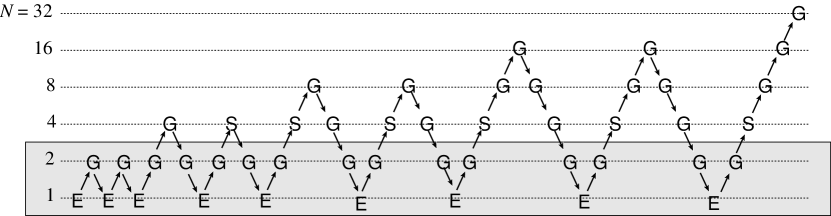
Figure 2: Schematic diagram of FMG scheme. The symbols G, S, and E denote the red-black Gauss-Seidel iteration, SOR, and solving an exact solution, respectively. The arrows directing right upward and right downward denote interpolation and restriction, respectively. In the hatched levels, the operations are done only in the $\ell=\ell_{\rm max}$.

We obtain an approximate solution on a finer nested grid successively by combination of interpolation, the red-black Gauss-Seidel iteration and restriction (averaging). We use the bilinear formula to interpolate the solution on a coarse grid for that on a fine grid. On the other hand we use the full weighting (the simple volume average) to restrict the solution on a fine grid to that on a coarse grid. We perform these operations on the order of the FMG. The schedule of the operations are schematically shown in Figure 2. The arrows directing right upward denote interpolation while those directing right downward do restriction. The symbol, G, denotes the red-black Gauss-Seidel iteration while the symbol, S, dose SOR. At the points of the symbol, E, an exact solution is given. The red-black Gauss-Seidel iteration is performed twice both after interpolation and interpolation in a typical model. In other words, the number of pre- and post-iterations is two in our computation.

Each restriction is performed by simply taking the average in the cells involved in a coarse cell. Restriction is done from fine ($\ell\,=\,\ell_{\rm max}$) to coarse ($\ell\,=\,1$).

Each interpolation is performed in the following procedures.

1. Fill the data in the region covered with a finer grid by the average value in the finer grid. This averaging is performed successively from $\ell\,=\,\ell_{\rm max}\,-\,1$ to $\ell\,=\,1$.

2. Perform linear interpolation of three dimensional data successively from $\ell\,=\,1$ to $\ell\,=\,\ell_{\rm max}$. The data on the boundary is given from the coarser grid.

Each red-black iteration is performed in the following procedures.

1. Obtain the gravitational potential just outside the grid level boundary using Equation (20).

2. Evaluate the gravity, $g$, on the cell boundary using Equations (14), (15), (16) and (19).

3. Replace the gravity at the grid level boundary with the fine grid using Equation (17).

4. Compute the residual in the red ($i\,+\,j\,+\,k$ = odd) cells and update the data there.

5. Repeat procedures 1 – 3.

6. Compute the residual in the black ($i\,+\,j\,+\,k$ = even) cells and update the data there.

The above procedures are counted as a cycle of the red-black Gauss-Seidel iteration.

The boundary condition was set only on the boundaries of the largest grid. We can use either the Dirichlet boundary (setting $\phi$ on the boundary) or the Neumann boundary (setting $g$). In the following we use the Neumann boundary. The gravity on the boundary was computed by the multi-pole expansion.

4 Sample Computation

We evaluate the efficiency of the above described algorithm with emphasis on the accuracy, convergence and computation time (load). In our numerical computation we take the unit, $G\,=\,1$, for convenience. All the numerical computations were done in the double precision.

4.1 Accuracy

First we present an example in which two uniform density spheres are placed near the center of the nested grid. The central positions, radii, and masses of the spheres are listed in Table 1. We obtained the gravitational potential for this mass distribution with the method mentioned in the previous sections. We used the nested grid of $N\,=\,64$, $L\,=\,1$, and $\ell_{\rm max}\,=\,5$. This example provides us the accuracy of our scheme.

We started the computation from the initial guess, $\phi\,=\,0$. The residual decreased by more than a factor of several hundreds by each FMG iteration. After 5 times iteration, the residual was of the order of the round off error ($\approx\,10^{-15}$ in the potential) as will be shown in §§4.2. The obtained gravitational potential is shown in Figures 3a, b, and c. Each panel denotes the contours of the gravitational potential measured in the midplane. As shown in Figure 3a, the gravitational potential $\phi$ has two local minima of which centers are close to the those of two spheres. It is well approximated by the $1/r$ potential in the region far from these spheres. These features ensure that the obtained solution is qualitatively correct.

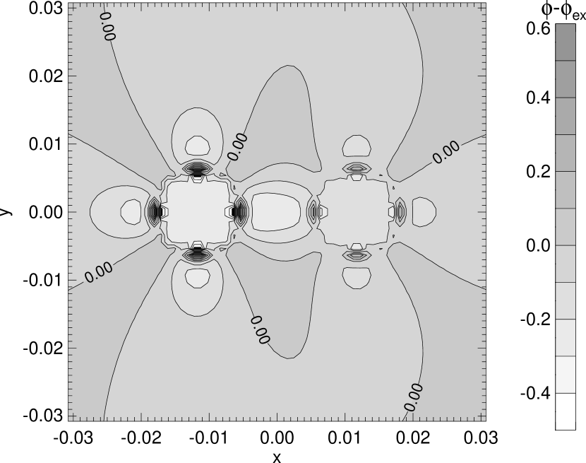
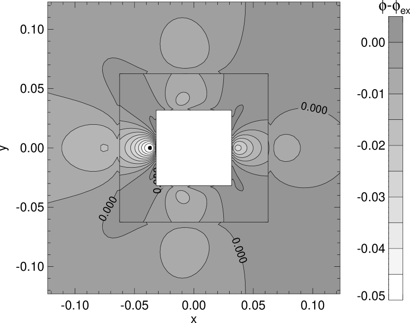
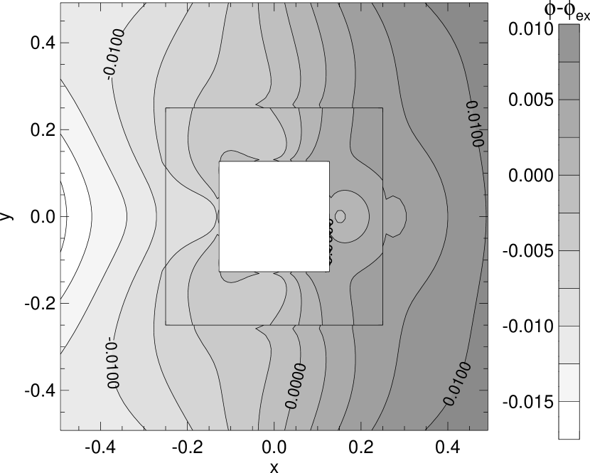
Figure 4: Errors of gravitational potential due to difference scheme for the example shown in Figure 3. The grayness and contours denote the difference form analytic solution ($\Delta\phi=\phi-\phi_{\rm ex}$). Panel (a) denotes the difference on $z\,=\,1/2048$ in the grid level of $\ell\,=\,5$. Panel (b) denotes that on $z\,=\,1/1024$ and 1/512 in the grid levels of $\ell\,=\,4$ and 3, respectively. Panel (c) denotes that on $z\,=\,1/256$ and 1/128 in the grid levels of $\ell\,=\,2$ and 1, respectively.

We compare the above solution with the exact analytic solution to examine the accuracy of our difference scheme. Figure 4a, b, and c denote the difference between the numerical and analytic exact solutions for the example shown in Figure 3. We do not show the difference in the region covered with a finer grid, since the numerical solution has no practical use there. Our numerically obtained $\phi$ has an arbitrary offset, since we used the Neumann boundary. The offset was chosen to minimize the difference between the numerical and analytic solution at $z\,=\,1023/2048$. On the grid of $\ell\,=\,5$, the difference is large ($|\Delta\phi|\,=\,0.6$) in the cells located near the surfaces of the spheres as shown in Figure 4a. This error is inevitable since it is due to the finiteness of our grids. It is, however, much smaller than the absolute value of the gravitational potential, of which maximum is $\max\,|\phi|\,=\,552.0$. The difference from the exact solution is typically as large as $|\Delta\phi|\,=\,0.1$ in the region covered with the grid of $\ell\,=\,5$.

The difference from the analytic solution is less than $|\Delta\phi|\,<\,0.016$ in the region covered with the grid of $\ell\,=\,3$ as shown in Figure 4b. The difference is relatively large near the grid level boundary between $\ell\,=\,3$ and 4. This is most likely due to the evaluation of the gravity at the grid level boundary. Our numerical scheme is the second order accurate except at the grid level boundaries since we employ the center difference. The gravity at the grid level boundary is only the first order accurate [see Eqs. (19) and (20)].

On the grid of $\ell\,=\,1$, the error is global; it is negative in the left ($x\,<\,0$) and positive in the right ($x\,>\,0$). This error comes from the boundary condition. We applied the Neumann condition for the outer boundary. The gravity at the boundary is evaluated by the multi-pole expansion in which we take account of the dipole, quadruple, and octuple moments as well as the total mass. These higher order moments and total mass are evaluated from the density distribution on the coarse grid of $\ell\,=\,1$. Thus even the dipole moment is seriously underestimated in this example. This underestimation is dominant in the error on the coarse grid $\ell\,=\,1$. The quadruple and octuple moments are practically not taken into account on the boundary in the example. If we apply a better outer boundary condition, the error will be reduced.

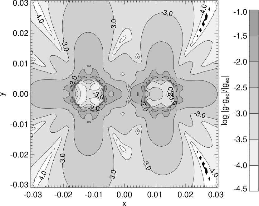
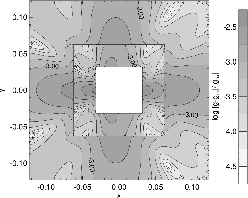
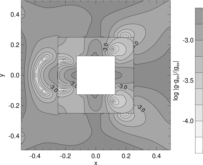
Figure 5: Same as Figure 4 but for relative errors of gravitational force ($|\mbox{\boldmath$g$}-\mbox{\boldmath$g$}_{\rm ex}|/|\mbox{\boldmath$g$}_{\rm ex}|$) in logarithmic scale.

Next we examine the accuracy of the gravity at the cell center, $\mbox{\boldmath$g$}_{i,j,k}$, defined by Equation (21). Figure 5 is the same as Figure 4 but for the relative error, $|\mbox{\boldmath$g$}\,-\,\mbox{\boldmath$g$}_{\rm ex}|/|\mbox{\boldmath$g$}_{\rm ex}$, where $\mbox{\boldmath$g$}_{\rm ex}$ denotes the exact gravity obtained analytically. The relative error is large ($\sim 0.1$) in the cells located on the surfaces of the spheres. It is much less than $10^{-2}$ in most cells. This small error ensures hat our scheme reproduces not only the $1/r$ potential but also the quadruple moment of the binary. The error is moderately large ($\sim 0.02$) in the cells adjacent to the grid level boundary. It is fairly small except in the cells located on the surfaces of the spheres. The large error on the surfaces of the spheres are due to the fact that even the finest grid is too coarse to resolve the surface sharply and not serious in practical use. In most hydrodynamical simulations, a self-gravitating gas has a more or less smooth density distribution in the finest grid.

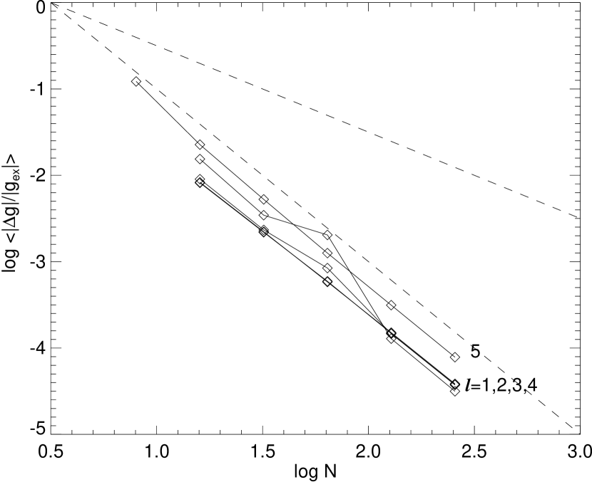
Figure 6: Errors of gravitational force as a function of $N$. The errors are evaluated as (a and b) simple averages, (c and d) root mean squares, and (e and f) maximum values of relative errors of gravitational force ($|\mbox{\boldmath$g$}-\mbox{\boldmath$g$}_{\rm ex}|/|\mbox{\boldmath$g$}_{\rm ex}|$). Panels (b), (d), and (f) denote the errors for cells on grid level boundaries while panels (a), (c), and (e) denote the errors for the other cells. Each solid curve denotes the error for each grid level ($\ell=1-\ell_{\rm max}$) as labeled in the panels. The dashed lines denote $10^{0.5}\,N^{-1}$ and $10\,N^{-2}$ for comparison.

To evaluate the relative error in the gravity quantitatively, we measured the simple average, the root mean square average, and the maximum value. Figure 6 show them as a function of $N$. The average and maximum are computed separately for cells adjacent to the grid level boundary and for the rest cells. Each curve denotes the value at the grid of each level. Panels b, d, and f are for the cells adjacent to the grid level boundary while panels a, c, and e are for the rest cells. Panels a and b show the simple average. Panels c and d show the root mean square average. Panels e and f show the maximum. The shallower dashed lines denote $|\mbox{\boldmath$g$}\,-\,\mbox{\boldmath$g$}_{\rm ex}|/|\mbox{\boldmath$g$}_{\rm ex}|\;=\;10^{-0.5}\,N^{-1}$ for comparison between panels. The steeper dashed lines denote $|\mbox{\boldmath$g$}\,-\,\mbox{\boldmath$g$}_{\rm ex}|/|\mbox{\boldmath$g$}_{\rm ex}|\;=\;10\,N^{-2}$.

In the cells not adjacent to the grid level boundary, the simple average and root mean square average of the relative error in the gravity are proportional to $N^{-2}$. The root mean square average are nearly as large as the simple average. The maximum value is only three times larger than the simple average at the levels of $\ell$ = 1, 2, 3, and 4. It is factor 10 larger than the simple average at $\ell\,=\,5$. These result confirm that our scheme gives the second order accurate gravity in the cells neither adjacent to the grid level boundary nor lying on the sharp edge of the density distribution.

In the cells adjacent to the grid level boundary, the relative error decreases in proportion to $N^{-1}$ except at $\ell\,=\,1$. This is because our scheme is only the first order accurate at the grid level boundary. This does not mean that the error is always large only at the grid level boundary. Note that the average relative error is more or less the same between in the cells adjacent to the grid level boundary and in the rest cells when $N\,\leq\,32$. Only when $N$ is sufficiently large, the error is appreciably large at the grid level boundary.

At $\ell\,=\,1$, the relative error decreases rapidly with increase in $N$. When $N\,\geq\,128$, the binary is resolved even in the grid of $\ell\,=1$. Then the dipole and quadruple moments of the gravity are evaluated with a good accuracy and the outer boundary condition is improved greatly. Accordingly the relative error is small at $\ell\,=\,1$ when $N\,\geq\,128$. Remember that the error due to the outer boundary condition dominates at $\ell\,=\,1$.

We made another example to confirm that our scheme can reproduce not only the $1/r$ gravity but also the quadraple moment of the gravity accurately. Figure 7 shows the second example in which 4 uniform density spheres are placed near the center of the grid. The centers, radii, and masses of the spheres are listed in Table 2. Note that the total mass is zero. When measured in the coarse grid of $\ell\,\leq\,2$, the cell average density vanishes in all the cells since $N\,=\,64$ in this example. In other words, there are no source terms in the discrete Poisson equation at the level of $\ell\,=\,1$. Nevertheless, the quadraple moment of gravity is reproduced in Figure 7. This proves that Equation (17) connects the gravitational potential between the coarse and fine grids.

4.2 Convergence

We measured reduction in the residual, the difference in the right and left hand sides of Equation (13), to evaluate the efficiency of the iteration. Figure 8 shows the residual as a function of the number of the FMG iteration cycle for the sample problem for binary shown in §§4.1. The absolute value of the residual reduces by a factor of 300 per one cycle of multi-grid iteration in the first four times of the FMG iteration. The residual remains constant after the five times FMG iteration. The remaining residual is due to the round off error in the gravitational potential. The residual is proportional to the inverse square of the cell size in Figure 8 since the second derivative is plotted. The round off error is extremely small and is negligible compared with the discretization error discussed in §§4.1.

Trying several model density distributions, we have confirmed that the reduction depends little on the spatial distribution of the residual.

When we increase the number of the Gauss-Seidel iteration during a cycle of the multi-grid iteration, we get a higher reduction in the residual per cycle at the expense of longer computation time. The reduction per unit computation load is higher when we the Gauss-Seidel iteration is performed several times each.

We tried the successive over relaxation (SOR) instead the Gauss-Seidel iteration to accelerate the converge but failed. When SOR is used as the pre- and post-relaxation in our multi-grid iteration, the residual increases sometimes depending on the initial guess. SOR works well only when use one level of the grid, i.e., when the grid is not nested.

We also tried to improve the interpolation formula, Equation (19), for a higher order accuracy. We found that our iteration did not converge when we used a higher order interpolation formula. Though we can not deny existence of a successful interpolation formula, we could not find it.

4.3 Computation Time

We evaluated the computation load of our multi-grid algorithm by measuring the computation time. A UNIX workstation, SGI O2 (MIPS R10000 250 MHz) was used for the measurement. The computation time was measured with the subroutine DTIME.

Figure 9 shows the execution time per FMG cycle. When The abscissa denotes the effective total number, $N_{\rm cell}$ = $\ell_{\rm max}\,N^{3}$, in the logarithmic scale. The ordinate denotes the logarithm of the computation time, $t$. The dashed lines denote the relations, CPU time $\propto\,N_{\rm cell}$ and CPU time. We made this plot by changing $\ell_{\rm max}$ and $N$ in the range of $2\,\leq\,\ell\,\leq\,10$ and $8\,\leq\,N\,\leq\,128$.

As shown in Figure 9, the computation load is proportional to the $N_{\rm cell}$ when $N\,\geq\,32$. This means that our algorithm is scalable for medium and large nested grids.

We also measured the computation time with the super computer Fujitsu VPP5000 at National Astronomical Observatory, Japan. When $N\,=\,256$ and $\ell_{\rm max}\,=\,5$, the CPU time is 0.21 sec per FMG cycle. This CPU time is reasonably small compared with the CPU time for solving the hydrodynamical equation on the same nested grid. This CPU time is not scalable to the number of cells since the super computer has vector processors and its CPU time is not proportional to the computation load.

5 DISCUSSIONS

As shown in the previous section, our numerical method provides an accurate solution with a reasonably small computation cost. The computation load is scalable in the sense that it is proportional to the number of the cells contained in the nested grid. Our discrete Poisson equation is robust in the sense that it can be applied also to AMR as far as a parent cell is subdivided into two in one dimension. We discuss the strength of our scheme while comparing with other schemes given in literatures.

Suisalu & Saar (1995) took another approach when solving the Poisson equation in their AMR computation. They adopted an cubic interpolation formula at the grid level boundary to ensure the continuity of the solution. They have noticed that a linear interpolation ensures only the continuity in the potential but not that in the gravitational force. Discontinuity in the force may cause a spurious feature across the grid level boundary. Although not mentioned explicitly in Suisalu & Saar (1995), the discontinuity causes a more serious problem; it introduces spurious mass on the grid level boundary. If the gravity $g$ has different values at a grid level boundary, the solution does not satisfies the Gauss’s theorem. The spurious mass on the grid boundary gives a serious error on the solution in a long range. The error decreases only inversely proportional to the distance from the spurious mass. This error dominates over the gravitational torque which decreases more steeply.

Compared with adoption of a higher order interpolation formula at the grid level boundary, our scheme has several advantages. First our approach ensures absence of a spurious mass on the grid level boundary while it is not guaranteed in a higher oder interpolation formula. Second higher order interpolation formula increases computation load. Third higher order interpolation may slow down efficiency of convergence. As far as in our experience, a simple multi-grid iteration does not work when Equations (19) and (20) are replaced with a higher order interpolation formula. We discuss the third point further in the following.

Our discrete Poisson equation has the following favorable character. When it is rewritten in the form,

$$\rho_{i}\;=\;\sum_{j}a_{i,j}\phi_{j}\;,$$ (22)

the coefficient $a_{i,j}$ is always positive except for $i$ = $j$. Here symbols $i$ and $j$ denote the cell number after sorted in one dimension. This property ensures that the Gauss-Seidel iteration converges always since it always underestimates the correction. In other words, the convergence of the Gauss-Seidel iteration is ensured since the matrix $a_{i,j}$ is diagonally dominant,

$$\sum_{i\neq j}|a_{i,j}|\;\leq\;|a_{i,i}|\;.$$ (23)

When we use a higher order interpolation formula, this the dominance of the diagonal element [Eq. (23)] is lost. The coefficient $a_{i,j}$ is no longer always positive. Then the Gauss-Seidel iteration may overestimate the correction and may not converge. If we apply successive under-relaxation, the convergence slows down.

Ricker et al. (2000) have proposed another idea for solving the Poisson equation in a nonuniform grid. They have used a nonuniform grid in which the spacing in a certain direction varies but only in the direction. For example, the spacing in the $x$-direction varies with $x$ but not in the $y$- and $z$-directions. Consequently each cell is rectangular and may have different side lengths. Each cell has a neighboring cell in each direction and faces 6 neighboring cells in total except for a cell located on the grid. They evaluated the gravity on the cell surface using the second order interpolation. Their Poisson equation can be rewritten as

$$\frac{g_{x,i+1/2,j,k}\,-\,g_{x,i-1/2,j,k}}{\Delta x_{i}}\,+\,\frac{g_{y,i,j+1/2,k}\,-\,g_{y,i,j-1/2,k}}{\Delta y_{j}}\,+\,\frac{g_{z,i,j,k+1/2}\,-\,g_{z,i-1/2,j,k-1/2}}{\Delta z_{k}}\,=\;4\pi G\rho_{i,j,k}\;,$$ (24)

where

$$g_{x,i+1/2,j,k}\;=\;F_{2,i}\phi_{i+2,j,k}\,+\,F_{1,i}\phi_{i+1,j,k}\,+\,F_{0,i}\phi_{i,j,k}\;$$ (25)

$$F_{2,i} = \frac{2\,(\Delta x_{i}\,-\,\Delta x_{i+1})}{(\Delta x_{i}\,+\,\Delta x_{i+1}\,+\,\Delta x_{i+2})\,(\Delta x_{i+1}\,+\,\Delta x_{i+2})}\,$$ (26)

$$F_{1,i} = -\,\frac{2\,[\Delta x_{i}^{2}\,-\,3\Delta x_{i+1}\,(\Delta x_{i+1}\,+\,\Delta x_{i+2})\,-\,\Delta x_{i+2}^{2}]}{(\Delta x_{i}\,+\,\Delta x_{i+1}\,+\,\Delta x_{i+2})\,(\Delta x_{i+1}\,+\,\Delta x_{i+2})\,(\Delta x_{i}\,+\,\Delta x_{i+1})}\;,$$ (27)

$$F_{0,i} = \frac{2\,(2\Delta x_{i+1}\,+\,\Delta x_{i+2})}{(\Delta x_{i}\,+\,\Delta x_{i+1}\,+\,\Delta x_{i+2})\,(\Delta x_{i}\,+\,\Delta x_{i+1})}\;.$$ (28)

The symbols, $\Delta x_{i}$, $\Delta y_{j}$, and $\Delta z_{j}$ denote the side length of each cell. We omitted the interpolation formula for $g_{y}$ and $g_{z}$ to save space. Integrating Equation (24) over the whole volume, we obtain

$$\sum_{i,j,k}\rho_{i,j,k}\,\Delta x_{i}\,\Delta y_{j}\,\Delta z_{k}\;=\;\sum_{i,j,k}H_{i,j,k}\phi_{i,j,k}\;,$$ (29)

where $H_{i,j,k}$ does not vanish in a nonuniform grid. This means that $\phi_{i,j,k}$ is not necessary to vanish even when $\rho_{i,j,k}$ = 0. In other words Equation (24) has multiple solutions for a given density distribution and boundary conditions. This is a serious problem.

As shown above, the approach based on a higher order interpolation formula has some fundamental problems. Although our scheme is only the first order accurate at the grid boundaries, it give a quantitatively good solution. This is likely to be due to the fact that our difference scheme satisfies global conditions for the proper Poisson equation to satisfy. First our scheme satisfy the Gauss’s theorem as mentioned repeatedly. Second our scheme ensures the Stokes’ theorem,

$$\oint\mbox{\boldmath$g$}\cdot d\mbox{\boldmath$s$}\;=\;0\;.$$ (30)

Equation (19) is equivalent to

$$\phi(\mbox{\boldmath$r$}_{1})\;=\;\phi(\mbox{\boldmath$r$}_{2})\;+\;\int_{1}^{2}\,\mbox{\boldmath$g$}\cdot d\mbox{\boldmath$r$}\;.$$ (31)

We adopted a principle that the difference equations should be consistent with the global properties, i.e., the Gauss’s theorem and Stoke’s theorem. We were satisfied with the first order accuracy at the grid level boundaries. In other words we gave priority to the global properties over the higher order accuracy at a given point. As a result we succeeded in computing the gravity of a close binary and in reproducing the quadraple moment. This success is analogous to that of a Total Variation Diminishing (TVD) scheme for wave equations and that of symplectic integrator for a Hamiltonian system (Yoshida, 1990). TVD scheme gives priority to monotonicity of the solution over the local accuracy (see, e.g. Hirsch, 1990). The solution is free from numerical oscillations. A symplectic integrator gives a solution which satisfies the conservation of the volume in phase space. As a result there is no secular change in the total energy, even though it is not conserved at each time step due to the limited accuracy. These examples confirm that the global properties are more important than the higher order accuracy.

An alternative method was proposed by Truelove et al. (1998). Their numerical scheme is based on that of Almgren et al. (1998) who solved the dynamics of an incompressible fluid with AMR. They evaluated the gravitational potential, $\phi$, not on the cell centers but on the vertexes. While they applied the cell centered difference to the hydrodynamical equations, they applied the vertex centered difference to the Poisson equation. This method has an advantage that the different level cells share the same gravitational potential automatically. In other words, this method ensures the continuity of the gravitational potential between the grids of different levels. This method, however, does not satisfies the Gauss’s theorem and accordingly does not ensure the continuity of the gravity, $g$.

The method of Truelove et al. (1998) has another disadvantage that it underestimates gravity. This disadvantage is due to averaging used to evaluate the vertex centered density. They evaluated the density at a vertex since the Poisson equation is evaluated on the vertex center. Averaging lowers the peak density and broadens the density distribution. Thus the gravitational potential evaluated at the vertex is shallower than that evaluated at the cell center. This difference is seriously large when the gas is concentrated in a few cells.

We have applied our Poisson equation solver to numerical simulations of binary star formation. The results will be published in near future.

Table 1: Mass distribution in model shown in Fig. 3

$n$	$x_{{\rm c},n}$	$y_{{\rm c},n}$	$z_{{\rm c},n}$	$r_{{\rm c},n}$	$M_{\rm n}$
1	12/1024	0	0	6/1024	1
2	$-$12/1024	0	0	6/1024	2

Table 2: Mass distribution in model shown in Fig. 7.

$n$	$x_{{\rm c},n}$	$y_{{\rm c},n}$	$z_{{\rm c},n}$	$r_{{\rm c},n}$	$M_{\rm n}$
1	2/1024	2/1024	0	2/1024	1
2	2/1024	6/1024	0	2/1024	$-1$
3	6/1024	2/1024	0	2/1024	$-1$
4	6/1024	6/1024	0	2/1024	1

Figure 3: Example of our numerical solution for gravitational potential of binary stars. Each component star of the binary is assumed to be a sphere of the uniform density. The centers, radii, and densities are summarized in Table 1. The contours denote the computed gravitational potential. It is measured in the plane of $z$ = 1/2048 at the level of $\ell\,=\,5$ in panel (a), in the plane of $z$ = 1/512 at the level of $\ell\,=\,3$ in panel (b), and in the plane of $z$ = 1/128 at the level of $\ell\,=\,1$ in panel (c). The contours are set in the equal interval in the logarithmic scale, $\Delta\log|\phi|\,=\,0.1$. The labels denote the values of $\log\,|\phi|$.

Figure 7: Gravitational potential computed for the density distribution in which four uniform density gas spheres are placed near the center of the computation grid. Two of them have positive mass and the other two have negative mass so that the gravitational field is well approximated by the quadraple in the region far from the center. The location and size of the four gas spheres are listed in Table 2. The contours are set in the equal interval in the logarithmic scale at the level of $\phi\,=\,\pm 10^{n}$ and 0 where $n$ denotes an arbitrary integer.

Figure 8: Residual of the Poisson equation ($\rho-\nabla^{2}\phi$) as a function of the number of the FMG iteration cycle ($N_{\rm FMG}$). Each curve denotes the maximum residual measured in the grid of each level. The dashed lines denote the relationships of $\rho-\nabla^{2}\phi\propto 10^{-2N_{\rm FMG}}$ and $10^{-3N_{\rm FMG}}$, respectively.

Figure 9: Computation time as a function of the number of the cells in the nested grid. The squares denote the computation time measured with the UNIX workstation, SGI O2 (MIPS R10000 250 MHz). The ordinate denotes the computation time, $t$, in unit of second in the logarithmic scale. The abscissa denotes the total number of the cells used in the nested grid, i.e., $N_{\rm cell}\,=\,{\ell_{\rm max}}\,N^{3}$, in the logarithmic scale. The parameters of the grid, ($N$, $\ell_{\rm max}$), are labeled by the filled squares. The relations of $t=10^{-6}N_{\rm cell}$ are drawn by the dashed lines for comparison.

References

- Almgren et al. (1998) Almgren, A. S., Bell, J. B., Colella, P., Howell, L. H., & Welcome, M. L. 1998, J. Comput. Phys., 142, 1
- Berger & Oliger (1984) Berger, M. J. & Oliger, J. 1984, J. Comput. Phys., 53, 484
- Burkert & Bodenheimer (1993) Burkert, A., & Bodenheimer, P. 1993, MNRAS, 264, 798
- Burkert & Bodenheimer (1996) Burkert, A., & Bodenheimer, P. 1996, MNRAS, 280, 1190
- Boss et al. (2000) Boss, A. P., Fisher, R. T., Klein, R. I., & McKee, C. F. 2000, ApJ, 528, 325
- Briggs, Henson, & McCormick (2000) Briggs, W. L., Henson, V. E., McCormick, S. F. 2000, A Multi Grid Tutorial, Second Ed. (Philadelphia: SIAM)
- Hirsch (1990) Hirsh, C. 1990, Numerical Computation of Internal and External Flows, Vol. 2 (Chichester: Wiley), 528
- Ricker et al. (2000) Ricker, P. M., Dodelson, S., & Lamb, D. Q. 2000, ApJ, 536, 122
- Norman & Bryan (1999) Norman, M. L. & Bryan, G. L. 1999, in ASSL Vol. 240, Proc. Numerical Astrophysics ed. S. M. Miyama, K. Tomisaka, & T. Hanawa (Dordrecht: Kluwer) 19
- Press et al. (1986) Press, W. H., Flannery, B. P., Teukolsky, S. A., & Vetterling, W. T. 1986, Numerical Recipes (Cambridge: Cambridge Univ. Press)
- Press & Teukolsky (1991) Press, W. H., & Teukolsky, S. A. 1991, Comput. Phys., 5, 514
- Suisalu & Saar (1995) Suisalu, I. & Saar, E. 1995, MNRAS, 274, 287
- Tomisaka (1998) Tomisaka, K. 1998, ApJ, 402, L163
- Truelove et al. (1997) Truelove, J. K., Klein, R. I., Mckee, C. F., Holliman, J. H., II, Howell, L. H., & Greenough, J. A. 1997, ApJ, 489, L179
- Truelove et al. (1998) Truelove, J. K., Klein, R. I., McKee, C. F., Holliman, J. H., II, Howell, L. H., Greenough, J. A., & Woods, D. T. 1988, ApJ, 495, 821
- Wesseling (1992) Wesseling, P. 1992, An Introduction to Multigrid Methods (Chichester: Wiley)
- Yoshida (1990) Yoshida, H. 1990, Physics Letters A, 150, 262