Far infrared observations of pre-protostellar sources in Lynds 183

Using ISOPHOT maps at 100 and 200 $\mu$m and raster scans at 100, 120, 150 and 200 $\mu$m we have detected four unresolved far-infrared sources in the high latitude molecular cloud L 183. Two of the sources are identified with 1.3 mm continuum sources found by Ward-Thompson et al. (wthompson94 (1994), wthompson00 (2000)) and are located near the temperature minimum and the coincident column density maximum of dust distribution. For these two sources, the ISO observations have enabled us to derive temperatures ($\sim 8.3$ K) and masses ($\sim$1.4 and 2.4 M_☉). They are found to have masses greater than or comparable to their virial masses and are thus expected to undergo gravitational collapse. We classify them as pre-protostellar sources. The two new sources are good candidates for pre-protostellar sources or protostars within L 183.

1 Introduction

Low-mass stars are known to form within dark clouds. To study the initial conditions for their formation, it is important to probe the physical conditions of both molecular gas and cold dust in the deep interiors of such clouds. Dense cores have been identified inside dark clouds, some probably being in the stage of contraction to form a star. A pre-protostellar core is defined as the stage in which a gravitationally bound core has formed in a molecular cloud, but no central hydrostatic protostar exists yet within the core (see e.g. Ward-Thompson et al. wthompson94 (1994)). Pre-protostellar cores are thought to be very cold. Thus, in many cases they escaped detection by IRAS, limited to $\lambda\leq 100\,\mu$m.

The long wavelength and multi-filter capabilities of ISOPHOT aboard the Infrared Space Observatory (ISO) (Kessler et al. kessler96 (1996)), combined with its improved sensitivity and spatial resolution over IRAS, have been utilized in studying the far-IR emission of molecular clouds and pre-stellar and young embedded stellar objects within them. Analysis of their physical parameters is facilitated by using the spectral energy distributions (SEDs) obtained from ISOPHOT multi-filter photometry.

1.1 Lynds 183

The dark cloud/large globule L 183, frequently cited also as L 134 North, is a prototypical dense cold molecular cloud. Its visual extinction is estimated to be $\sim 17^{\mathrm{m}}$ based on its 200 $\mu$m optical depth (Juvela et al. juvela02 (2002)). So far there is no evidence for associated newly born stars such as T Tauri stars or IRAS point sources. However, Martin & Kun (martinkun (1996)) have found a bona fide T Tauri star and H$\alpha$ emission line star near L 183. These two stars are located outside our maps. Given its short distance of $\sim$ 110 pc (Franco franco (1989)) L 183 provides a good spatial resolution with the ISO FIR beam size (ISOPHOT’s spatial resolution of 45$\arcsec$ at 100 $\mu$m corresponds to 0.02 pc at the distance of L 183). The location at high Galactic latitude ($b=36$ deg) minimizes contamination with unrelated cirrus along the line of sight. The location off the Galactic plane at $z=65$ pc implies that the impinging ultraviolet radiation field is strongly asymmetrical.

A Digitized Sky Survey red plate (’Equatorial Red’ survey (UK Schmidt) IIIaF + RG610) image of L 183 is shown in Fig. 1. In Fig. 1b, the original image has been smoothed with a FWHM=9″(nine image pixels) Gaussian kernel. The cloud has a dark core - bright rim structure, which is characteristic of clouds having high optical depth at visual wavelengths that are illuminated by the diffuse interstellar radiation field (Mattila mattila74 (1974); FitzGerald et al. fitzgerald76 (1976)). The bright rim maximum occurs at a radius corresponding to extinction A${}_{\lambda}\approx 1.5^{\mathrm{m}}-2^{\mathrm{m}}$.

Laureijs et al. (laureijs91 (1991)) observed the 60 $\mu$m emission to decline relative to 100 $\mu$m emission in a narrow transition layer around the cloud edge. They explained this behaviour by assuming a separate grain component at 60 $\mu$m that undergoes a modification of properties in a transition layer.

Laureijs et al. (laureijs95 (1995)) have used IRAS images, CO molecular line observations and blue extinction values from star counts for a large-scale study of the L 134 cloud complex, including L 134, L 169 and L 183. Using ¹³CO observations, they found 18 clumps in the complex and derived their properties. The clumps follow clear size vs. linewidth and luminosity vs. size relationships. An analysis and discussion of the dust and molecular gas properties in L 183 based on the ISOPHOT 100 and 200 $\mu$m emission maps has recently been presented by Juvela et al. (juvela02 (2002)).

L 183 has been a favourite target for molecular line observations which have revealed it as a rich source of molecular species (see e.g. Swade 1989a , 1989b ; Dickens et al. dickens (2000)). Lee et al. (lee01 (2001)) have classified L 183 as a strong infall candidate. The optically thick CS($J$=2-1) lines in the inner region of the cloud show a double peak with the blue component brighter than the red one, which is characteristic of inward motions. Similar profiles suggesting infall motions have been observed for HCO⁺($J$=3–2) (Gregersen & Evans gregersen00 (2000)) and for CS($J$=2–1) by Snell et al. (snell82 (1982)).

Mapping of the millimetre and submillimetre continuum dust emission by Ward-Thompson et al. (wthompson94 (1994), wthompson99 (1999)) has revealed a small extended core in the center of L 183. This source has been detected at 800, 1100 and 1300 $\mu$m, and has FWHM dimensions of $60\arcsec\times 40\arcsec$ (0.032 $\times$ 0.021 pc) at 800 $\mu$m. According to Ward-Thompson et al. (wthompson94 (1994)), the core is probably pre-protostellar in nature, i.e. at an earlier stage than an accreting Class 0 protostar (for the definition of a Class 0 object see André et al. andre93 (1993)). The submillimetre emission from the core is consistent with the dust being heated externally by the general interstellar radiation field. Recent observations by Ward-Thompson et al. (wthompson00 (2000)) have revealed that the continuum emission extends further to the south, and that there is another emission maximum located at a position about 1.5$\arcmin$ south of the previously detected maximum, with a FWHM size of $120\arcsec\times 60\arcsec$. From sub-mm polarization observations Ward-Thompson et al. (wthompson00 (2000)) measured a magnetic field direction which is at an angle of $34\degr\pm 6\degr$ to the minor axis of the core, and found evidence for decreasing polarization at the highest continuum emission intensities.

Ward-Thompson et al. (2002a ) have mapped the core of L 183 at 90, 170 and 200 $\mu$m with ISOPHOT. The core was not detected at 90 $\mu$m wavelength. The dust temperature derived from 170 and 200 $\mu$m data showed no temperature gradient across the core.

In this study, we search for pre- and protostellar objects in the cloud. Our maps are much bigger than previous (sub)millimetre continuum maps. The derived fluxes of the sources between 120–200 $\mu$m, located near the peak or in the Wien regime of the assumed blackbody radiation, are essential for temperature and thus mass determination of the objects. Only if the masses of the objects are determined can we study their dynamical state. Furthermore, we study the relation of young (proto)stellar objects with the properties of the underlying dust in the cloud such as temperature and column density.

In the context of L 183, the term ’pre-protostellar core’ has been previously used to refer to the two known (sub)mm continuum sources within the cloud (Ward-Thompson et al. wthompson94 (1994), wthompson00 (2000)), and also to the cloud core itself in which these sources are embedded (Ward-Thompson et al. 2002a ). Throughout this article, we use the term ’source’ to refer to objects in L 183 which are unresolved in our maps, such as the previously-known continuum sources. By the term ’core’, we refer to the visually opaque cloud core which is larger than the sources within it and resolved by ISO observations.

2 Observations and data reduction

Figure 1: Optical red Digitized Sky Survey (DSS) (a,b), 200 $\mu$m (c) and 100 $\mu$m (d) images of L 183. The four unresolved sources are marked as blue dots; for identification see Fig. 3. a) Digitized Sky Survey red plate. The image is scaled to best show the opaque core of the cloud. b) Digitized Sky Survey red plate. The image is scaled to best show details of faint surface brightness. c) False-colour image of 200 $\mu$m surface brightness. The colour scale is in units of MJy sr^-1. d) False-colour image of 100 $\mu$m surface brightness. Zodiacal light of 4.0 MJy sr^-1 has been subtracted. The colour scale is in units of MJy sr^-1

Table 1: The properties of filters. $\lambda_{\mathrm{ref}}$ is the reference wavelength, $\Delta\lambda$ is the width, and d_Airy is the diameter of the Airy disk

Filter	$\lambda_{\mathrm{ref}}$	$\Delta\lambda$	dAiry	Pixel size
	[$\mu$m]	[$\mu$m]	[$\arcsec$]	[$\arcsec$]
C_100	100	43.6	83.9	43.5$\times$43.5
C_120	120	47.3	101	89.4$\times$89.4
C_135	150	82.5	113	89.4$\times$89.4
C_200	200	67.3	168	89.4$\times$89.4

Table 2: The parameters of the observations. TDT is the Target Dedicated Time number of the observation, P.A. is the position angle measured from North to East. All observations were made on January 19th 1997

Filter	TDT	Raster steps	Map size	Grid	P.A.	Remarks
			[$\arcmin$]	[$\arcsec$]	[°]
C_100	43001032	14$\times$20	31.5$\times$30.8	135, 90	21.1	Map
C_200	43001031	10$\times$10	30.0$\times$30.0	180, 180	21.1	Map
C_100	43000411	13$\times$2	39$\times$3	180, 90	179.0	N-S stripe
C_120	43000413	10$\times$2	30$\times$3	180, 90	179.0	N-S stripe
C_135	43000412	10$\times$2	30$\times$3	180, 90	179.0	N-S stripe
C_200	43000414	10$\times$2	30$\times$3	180, 90	179.0	N-S stripe

The observations were made with the ISOPHOT instrument aboard the ISO satellite, using the C100 and C200 detectors (Lemke et al. lemke96 (1996)). We have mapped $\sim 30\times 30$ arc min² of the cloud at 100 and 200 $\mu$m. In addition, we have performed linear north-south raster scans at 100, 120, 150 and 200 $\mu$m through the cloud core with a two way path, the return path being shifted by 90$\arcsec$ to the west (see Fig. 3 for the raster scan positions and the orientation of the detector array). The raster scans were designed to cross the continuum source FIR 1. All observations were made using the observing template PHT22 in raster mode. Details of the detector/filter combinations and observational parameters are given in Tables 1 and 2.

The data analysis was done using PIA (ISOPHOT Interactive Analysis) V 8.1 (Gabriel et al. gabriel (1997)). At the first processing level, the detector ramps were corrected for non-linearity of the detector response, glitches in ramps were removed by using the two-threshold glitch recognition method, and the ramps were fitted with 1st order polynomials. At subsequent levels the signals were deglitched, reset interval correction was applied, signals were linearized for the dependence of detector response on illumination, and orbital position-dependent dark currents were subtracted.

For the flat-field correction, a statistical method was applied: the value of the reference pixel at each raster position was correlated with other pixels. Instead of comparing the reference pixel only with pixels located at the same raster position, a mean of two pixels located symmetrically around the reference pixel wass taken. In this way, it is possible to reduce the scatter caused by surface brightness gradients in the image.

The primary intensity calibrators are the fine calibration source (FCS) measurements, which bracket the actual map or raster scan measurements. The C100 detector suffers from response transients during the relatively short measurement time of the FCS. We have corrected for this effect by modelling the signal transients with the PIA signal drift interface, using the offset exponential as the fitting function. The C200 detector reacts faster, thus there is no such transient behaviour.

We have compared our 100 $\mu$m surface brightness calibration with COBE/DIRBE data. To match our data to the much coarser DIRBE resolution (0.7°$\times$0.7°), we have used the IRAS/ISSA 100 $\mu$m map of the L 183 area as an intermediate step (for the method see Lehtinen et al. lehtinen01 (2001)). We have thus found a scaling factor $I\mathrm{{}_{100\,\mu m}(ISOPHOT)}/I\mathrm{{}_{100\,\mu m}(DIRBE)}=1.25$. Although this value is well within the combined uncertainty of the absolute accuracies cited for ISOPHOT (20%, see Klaas et al. klaas00 (2000)) and for DIRBE (11%, see Hauser et al. hauser98 (1998)) it is larger than the scaling factor obtained for a sample of five mappings of different clouds where the ISOPHOT and DIRBE 100 $\mu$m surface brightnesses agree to within 15% (Lehtinen et al. lehtinen01 (2001)). We have thus rescaled our present ISOPHOT 100 $\mu$m map dividing it by 1.25 to correspond to the DIRBE calibration. The North-South raster scan data at 100 $\mu$m are scaled to the map.

A direct ISOPHOT vs. DIRBE comparison was done at 200 $\mu$m by averaging the ISOPHOT surface brightness over our whole map area and comparing it with the nearest DIRBE pixel value. The resulting scaling factor was 0.90, i.e. well within the uncertainties of each instrument. No rescaling was applied to our ISOPHOT data at 200 $\mu$m, nor at 120 and 150 $\mu$m.

3 Results

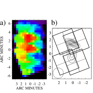
Figure 2: (a) Map made from the 200 $\mu$m stripe scan data. The pixel size is 30″. We note that this map is just to illustrate that the two continuum sources detected by Ward-Thompson et al. (wthompson94 (1994), wthompson00 (2000)) can be detected as separate sources in the stripe scan data. The details in this map are smaller than the actual resolution of the stripe scan data. (b) The model at 200 $\mu$m used to derive the fluxes of FIR 1 and FIR 2. The positions and sizes of the sources are those given by Ward-Thompson et al. (wthompson94 (1994), wthompson00 (2000)). The inclined boxes show the locations of the 2$\times$2 pixel C200 detector array in the North-South stripe scan. The contours of the continuum sources go from 0.8 to 6.4 in steps of 0.8 Jy pixel^-1. The FWHM of the ISO beam at 200 $\mu$m is shown at lower left hand corner. The center position in both maps is the position of FIR 2 (see Table 3)

Figure 3: Contour maps of 100 $\mu$m (a) and 200 $\mu$m (b) surface brightness. The detected unresolved sources are marked with asterisks. The additional raster scan positions (center of the detector array) observed at 100, 120, 150 and 200 $\mu$m are indicated by dots. The orientation of the C100 and C200 detector is shown for four raster scan positions. The sizes of the C100 and C200 detector pixels are shown at the upper right corners. a) The contours are from 12 to 23 MJy sr^-1 in steps of 1 MJy sr^-1. Zodiacal light of 4.0 MJy sr^-1 has been subtracted. b) The contours are from 20 to 85 MJy sr^-1 in steps of 5 MJy sr^-1. The chance location of FIR 3 within the detector area is shown

Figure 4: Profiles along image rows and columns through the sources FIR 3 and 4 at 200 $\mu$m. The solid line is a fit to the background, the dotted line shows the fitted point source profile. The vertical line shows the fitted position of the source

Figure 5: The spectral energy distributions of the unresolved sources. The 100, 120, 150 and 200 $\mu$m flux density values are our ISOPHOT measurements, others are from the literature. All fluxes are total fluxes (see Sect. 3.2). The solid lines are modified blackbody fits ($\beta=2$) to the data points. a) FIR 1. Derived temperature T=8.4 K. The dotted lines are blackbodies which have 1 K higher and lower temperatures than the solid line, demonstrating the accuracy of the derived temperature. b) FIR 2. Derived temperature T=8.2 K. c) FIR 3. Derived temperature T=12.8 K. d) FIR 4. The solid line is a modified blackbody curve (T=12.9 K), with a temperature equal to the colour temperature derived from the 100 and 200 $\mu$m flux densities

Table 3: Positions, sizes, and non colour-corrected total flux densities of unresolved sources in L 183. The 1-$\sigma$ error values for the flux densities include an estimated 50% error for FIR 1 and 2 and 30% error for FIR 3 and 4

Name	FWHM size	Position		Fν(100 $\mu$m)	Fν(120 $\mu$m)	Fν(150 $\mu$m)	Fν(200 $\mu$m)	Remarks
	[″]	$\alpha$(1950)	$\delta$(1950)	[Jy]	[Jy]	[Jy]	[Jy]
FIR 1	60$\times$40	$15^{\rm h}51^{\rm m}32\aas@@fstack{s}7$	$-2\degr 42\arcmin 19\arcsec$	-	0.14$\pm$0.07	0.76$\pm$0.38	2.6$\pm$1.3	1
FIR 2	120$\times$60	$15^{\rm h}51^{\rm m}33\aas@@fstack{s}0$	$-2\degr 44\arcmin 00\arcsec$	-	0.59$\pm$0.30	2.3$\pm$1.2	5.2$\pm$2.6	1
FIR 3		$15^{\rm h}51^{\rm m}33\aas@@fstack{s}6$	$-2\degr 49\arcmin 25\arcsec$	-	1.6$\pm$0.5	4.2$\pm$1.4	5.3$\pm$1.8
FIR 4		$15^{\rm h}51^{\rm m}48\aas@@fstack{s}4$	$-2\degr 46\arcmin 00\arcsec$	$<$0.6	-	-	4.7$\pm$1.6

¹Sizes and positions from Ward-Thompson et al. (wthompson94 (1994), wthompson00 (2000))

Table 4: The parameters for unresolved sources. T_d is the dust temperature. $\lambda_{0}$ is the wavelength (corresponding to $\nu_{0}$) where the optical depth is unity. The sub-mm luminosity L_sub-mm is the luminosity of the fitted blackbody function, integrated longward of 350 $\mu$m. L_bol is the bolometric luminosity, N(H₂) is the mean molecular hydrogen column density, and n(H₂) is the mean number density assuming a constant density sphere with size equal to the geometric mean of the minor- and major-axis FWHM sizes. M is the total (gas plus dust) mass, and M_vir is the virial mass. The quoted errors are 1-$\sigma$ errors based on Monte Carlo error estimation, including the estimated errors of fluxes only. Note that the parameters of FIR 3 have been calculated by assuming that its size is equal to the mean value of the sizes of FIR 1 and 2

Name	Td	$\lambda_{0}$	Lsub-mm	Lbol	$\frac{L_{\mathrm{sub-mm}}}{L_{\mathrm{bol}}}$	N(H2)	n(H2)	M	Mvir
	[K]	[$\mu$m]	[L☉]	[L☉]		[1022 cm-2]	[106 cm-3]	[M☉]	[M☉]
FIR 1	8.4$\pm 0.4$	63$\pm 6$	0.014	0.036	0.4	14	2.6	1.4	0.4
FIR 2	8.2$\pm 0.4$	48$\pm 8$	0.022	0.056	0.4	8.1	0.9	2.4	0.7
FIR 3	12.8$\pm 1.5$	12$\pm 5$	0.004	0.034	0.1	0.4	0.05	0.2
FIR 4	$<$12.9			$<$0.05				-

3.1 Unresolved sources in L 183

The ISOPHOT far-IR maps at 100 $\mu$m and 200 $\mu$m, together with optical images, are shown in Fig. 1. We have searched for point-like objects by visual inspection. Neither one of the sub-mm continuum sources detected by Ward-Thompson et al. (wthompson94 (1994), wthompson99 (1999), wthompson00 (2000)) is detected in the 100 $\mu$m map (see Fig. 1d). At 200 $\mu$m there is an emission maximum at the position of the sources (see Fig. 1c). They have an angular distance of $\sim$1 pixel, so they are not detected as separate sources in the 200 $\mu$m map. However, in the C200 North-South stripe scans the resolution is better due to overlapping pixels (see Fig. 2b). A map made from the 200 $\mu$m stripe scan data clearly shows two emission maxima whose positions correspond to positions of the continuum sources of Ward-Thompson et al. (see Fig. 2a). In order to derive the total fluxes of these sources, our sources FIR 1 and 2, we have modelled them by two-axial gaussian surfaces having position angles and FWHM sizes as given by Ward-Thompson et al. (wthompson94 (1994), wthompson00 (2000)). We have not made a 2-D map of the stripe scan data, but have treated them as a 1-D time-ordered data for each pixel. The background has been determined by fitting the 1-D data with cubic splines, excluding the positions where the sources contribute to the flux. The flux seen by each pixel has been calculated by using our 2-D model and ISO beam profile. The fluxes of the sources have been determined by minimizing the difference between the modelled and observed fluxes in a least squares sense. The model is shown in Fig. 2b, and the derived total fluxes are given in Table 3. The accuracy of the derived fluxes is mainly limited by our ability to subtract the strongly-varying background at the edge of the cloud. We therefore give an estimated error of $\pm 50$ % for the fluxes.

A visual inspection of the 200 $\mu$m map further reveals two previously unknown unresolved sources in the cloud, sources FIR 3 and 4 (see Fig. 1c). Neither of them is detected in the 100 $\mu$m map. FIR 3 is by chance located within the C200 detector array at one stripe scan position (see Fig. 3 b), which enables us to also estimate its flux at 120 and 150 $\mu$m. We take the flux of the pixel closest to the source, subtract from that the mean of the other three pixels, and correct the flux by the point spread function fraction for a point source centered on a pixel (Laureijs laureijs99 (1999)). An error of 30% has been estimated for the fluxes. The 5.3 Jy 200 $\mu$m total flux derived this way is in good agreement with the 5.8 Jy flux derived from the map. Profiles through FIR 3 along image rows and columns in the 200 $\mu$m map are shown in Fig. 4c and d, respectively.

Source FIR 4 is a prominent unresolved source on the 200 $\mu$m map (Figs. 1c and 4). On the 100 $\mu$m map there is an extended brightness enhancement around the position of FIR 4 (Fig. 1 d), where the 100 $\mu$m brightness reaches its maximum. In order to derive the 100 $\mu$m flux density, we have first convolved the data to the 200 $\mu$m resolution. Since it is difficult to separate the source from the structured background, we consider the derived flux density as an upper limit. Profiles through FIR 4 along image rows and columns in the 200 $\mu$m map are shown in Fig. 4a and b, respectively.

We have searched in the IRAS Point Source (PSC) and Faint Source Catalogs (FSC) for sources within our maps. We find two PSC sources, IRAS 15522–0258 and 15523–0251, and one FSC source, F15507-0245. None of them are detected by us. The IRAS sources are located outside the cloud centre. The PSC sources only have 100 $\mu$m IRAS fluxes. In the ISO maps, there is no enhancement of 100 $\mu$m surface brightness at the position of the PSC sources. As the ISO and IRAS images at 100 $\mu$m appear morphologically similar, it seems that the two 100 $\mu$m PSC sources are artefacts, and are a result of IRAS scanning direction with respect to structures in the cloud. The FSC source has a 12 $\mu$m detection only and is thus not expected to be detected at 100 $\mu$m.

3.2 The spectral energy distributions

At $\lambda\ga 100\,\mu$m, the emission arises from ’classical’ large grains, which are at an equilibrium temperature within the radiation field. We have thus fitted the flux densities at these wavelengths with a modified blackbody of the form

$$F_{\nu}=B_{\nu}(T_{\rm d})\,(1-\exp(-\tau_{\nu}))\,\Omega_{\rm s}$$ (1)

where $B_{\nu}(T_{\mathrm{d}})$ is the Planck function at the dust temperature $T_{\mathrm{d}}$, $\tau_{\nu}$ is the optical depth which is assumed to vary with frequency as $\tau_{\nu}=(\nu/\nu_{0})^{\beta}$, $\Omega_{\mathrm{s}}$ is the solid angle of the emitting region, and $\nu_{0}$ is the frequency at which the optical depth is unity. We have assumed that the emissivity index ${\beta}$ is 2. For the source size $\Omega_{\mathrm{s}}$ of FIR 1 and 2 we have used the FWHM sizes given by Ward-Thompson et al. (wthompson94 (1994); wthompson00 (2000)). The size of FIR 3 is unknown, so we have assumed a size which is a mean value of the sizes of FIR 1 and 2.

The 100 to 200 $\mu$m total fluxes measured with ISO are complemented by values at longer wavelengths from Ward-Thompson et al. (wthompson94 (1994); wthompson99 (1999)) for FIR 1, and from Ward-Thompson et al. (2002b ) for FIR 2. Ward-Thompson et al. (wthompson94 (1994)) give the total flux of FIR 1 only at 800 $\mu$m. From the given total flux and flux within a 18″beam we derive their ratio of 10.4. Because the other fluxes at 450 and 1100 $\mu$m are given for the same 18″beam as the 800 $\mu$m flux, we can use the ratio 10.4 to derive total fluxes. This way we derive total fluxes of $<$15.6 and 1.1 Jy at 450 and 1100 $\mu$m, respectively. Ward-Thompson et al. (wthompson99 (1999)) have given for FIR 1 at 1.3 mm a flux of 40 mJy within 13″beam. Thus the total flux is $(18/13)^{2}\times 10.4\times 40$ mJy=0.8 Jy. The spectral energy distributions and fitted modified blackbody functions for FIR 1, 2, 3 and 4 are shown in Fig. 5. The resulting temperatures are listed together with other parameters in Table 4. The uncertainties of the fitted parameters have been estimated by Monte Carlo methods.

For FIR 1, 2 and 3 the ISO flux densities, determined near the peak of the SEDs, accurately set the temperatures of the fitted blackbodies, as demonstrated in Fig. 5. The fitted temperatures are 8.4, 8.2 and 12.8 K, respectively. The derived colour temperature of FIR 4 has an upper limit of about 13 K. We note that the use of a single temperature is a simplification, and that the source sizes may be different at different wavelengths. Ward-Thompson et al. (2002a ) derived a temperature of 10$\pm 3$ K within a 150″circular core area of the cloud, which is within errors equal to our value, $8.3\pm 0.4$ K.

3.3 The luminosities, column densities, number densities, and masses of unresolved sources

The bolometric luminosities, L_bol, have been derived for all sources by integrating over the fitted blackbody curves (Table 4). For the bolometric luminosity of the core of the cloud Ward-Thompson et al. (2002a ) derived 0.15 L_☉ by integrating the fluxes at 170 $\mu$m and 200 $\mu$m in a circular 150″aperture, combining these fluxes with mm/submm fluxes, and fitting the SED with a modified blackbody. The combined luminosity of IRS 1 and 2 derived by us, 0.09 L_☉, is in excellent agreement with the core luminosity of Ward-Thompson et al. when taking into account the different distances used by us (110 pc) and Ward-Thompson et al. (150 pc).

The mean column densities through FIR 1 and 2 have been derived from the equation

$$N({\mathrm{H}}_{2})=F_{\nu}/\left(\Omega_{\mathrm{s}}\,\mu\>m_{\mathrm{H}}\,\kappa_{\nu}\,B_{\nu}(T_{\mathrm{d}})\right)$$ (2)

where $F_{\nu}$ is the observed flux, $\mu=2.33$ is the mean molecular weight, $m_{\mathrm{H}}$ is the mass of atomic hydrogen, and $\kappa_{\nu}$ the dust opacity per unit mass (gas+dust) column density (see e.g. Hildebrand hildebrand (1983); Chini et al. chini87 (1987)). We have adopted $\kappa_{1300\,\mu\rm{m}}=0.005$ cm² g^-1 which is valid for pre-protostellar dense clumps (Motte et al. motte98 (1998) and references therein), assuming a gas-to-dust ratio of 100. The value of $\kappa_{1300\,\mu\rm{m}}$, and correspondingly the column density, is uncertain by a factor of $\sim$2 (see e.g. Motte et al. motte98 (1998)). We obtain the values $N({\mathrm{H}_{2}})\approx 14\,10^{22}$ cm^-2 and 8.1 $10^{22}$cm^-2 for FIR 1 and 2, respectively. These values are similar to the values in cloud cores found by Motte et al. (motte98 (1998)) in $\rho$ Ophiuchi cloud based on millimeter continuum mapping, or by Bacmann et al. (bacmann00 (2000)) based on ISOCAM absorption survey. The difference by a factor of about two in the column density of IRS 1 between us and Ward-Thompson et al. (wthompson99 (1999)) is due to the higher temperature (12.5 K) adopted by Ward-Thompson et al.

Mean number densities $n$(H₂), assuming a constant density, have been calculated using the formula $n({\mathrm{H}_{2}})=(3/4)N({\mathrm{H}_{2}})/R$, where the cloud radius $R$ for FIR 1 and 2 is assumed to be the geometric mean of the minor- and major-axis FWHM sizes.

We are able to derive improved mass estimates because ISOPHOT flux values enable accurate determination of dust temperature. In order to estimate the total (gas plus dust) mass $M$ of matter associated with dust we use the equation

$$M=\frac{F_{\nu}D^{2}}{\kappa_{\nu}B_{\nu}(T_{\rm d})}$$ (3)

with $D$ the distance. The fitted values of $\lambda_{0}$, i.e. the wavelength where $\tau_{\rm dust}=1$ (see Table 4), suggest that for all sources the emission is optically thin at wavelengths $\ga 100\,\mu$m. For FIR 1, we have used the 1300 $\mu$m flux in Eq. (2), giving $M\approx 1.4$ M_☉. For sources FIR 2 and 3, we are using the 850 and 200 $\mu$m fluxes, respectively. The value of $\kappa_{\lambda}$ has been scaled from $\kappa_{1300\,\mu\rm{m}}$ by using a $\lambda^{-2}$ dependence. The derived masses of FIR 2 and 3 are 2.4 and 0.2 M_☉, respectively.

The relative mass of the sources can be derived without the knowledge of $\kappa_{\lambda}$ or $D$. Only the dust temperature and flux at any optically thin wavelength are required. We have derived the relative mass between FIR 1 and 2 using the optically thin 1.3 mm fluxes from the blackbody fit. The derived mass ratio between FIR 1 and 2 is 0.6.

3.4 Extended dust emission

Figure 6: Dust temperature as derived from the 100 and 200 $\mu$m maps. The unresolved sources have been removed from the 200 $\mu$m map before temperature calculation. The contours are from 11.4 to 14.2 in steps of 0.4 K. The detected sources are marked as stars. The temperature is not determinable outside the cloud due to the background subtraction. The size of the C200 detector is shown at the upper left corner

Figure 7: Map of beam-averaged optical depth at 200 $\mu$m after subtraction of the 4 point sources. The contours are from 1$\times 10^{-3}$ to 7$\times 10^{-3}$ in steps of 1$\times 10^{-3}$

A detailed analysis of the extended dust emission is presented by Juvela et al. (juvela02 (2002)). In this paper we will present the derivation of the temperature and column density distribution of the dust.

The deep red Schmidt image in Fig. 1 shows faint surface brightness details across the core, which are probably structures in front of the dense core and are seen as bright regions due to scattered light. In the optical image, the eastern part of the cloud is covered by diffuse material. The dense part of the cloud which is delineated by the background stars extends untill $\alpha\approx 15^{\mathrm{h}}52^{\mathrm{m}}$. Outside the diffuse material in the northern and western parts of the cloud the optical edge of the cloud closely follows the edge of 200 $\mu$m surface brightness. The region of strong ($\ga 80$ MJy sr^-1) 200 $\mu$m emission extends east behind the diffuse emission and follows the opaque cloud boundary. The diffuse emission is located in front of the cloud core.

There is a major difference between the 100 and 200 $\mu$m maps: the 200 $\mu$m maximum around the sources FIR 1 and 2 has no counterpart at 100 $\mu$m, i.e. there is a 200 $\mu$m emission excess relative to 100 $\mu$m. This could be due to a low dust temperature. Other explanations are that the dust emissivity at 200 $\mu$m increases in the dense core due to grain coagulation (Cambrésy et al. cambresy01 (2001); Stepnik et al. stepnik02 (2002)), or that the two wavelengths trace different dust populations.

In order to derive the colour temperature of dust, the fluxes at 100 and 200 $\mu$m have been fitted with a modified blackbody function of the form

$$I_{\nu}\propto\nu^{\beta}B_{\nu}(T_{\mathrm{d}})$$ (4)

where $\beta$ is the emissivity index and $T_{\mathrm{d}}$ is the dust temperature. We convolve the 100 $\mu$m map to the 200 $\mu$m resolution, and subtract the background (determined at the upper right corner in Fig. 3c and d). While fitting the modified blackbody, we iteratively make colour corrections until the difference between subsequent temperatures is less than 0.1 K. The temperature map (using $\beta=2$) is shown in Fig.6. The minimum at the center of the cloud is $T_{\mathrm{d}}\approx$11.1 K.

In the optically thin regime, the optical depth is given by observed surface brightness

$$\tau_{\nu}=I_{\nu}/B_{\nu}(T_{\mathrm{d}})$$ (5)

The map of beam-averaged optical depth at 200 $\mu$m is shown in Fig.7. The optical depth sharply decreases north of the sources FIR 1 and 2, while the decrease towards the south is smoother, similar to the morphology of the 200 $\mu$m map (Fig. 3 c). The highest optical depth, $\tau_{\mathrm{200\,\mu m}}\approx 7\times 10^{-3}$, is ten times larger than the optical depth through the center of the Thumbprint Nebula (Lehtinen et al. lehtinen98 (1998)), a globule without star formation.

4 Discussion

4.1 Are FIR 1 and 2 gravitationally bound objects ?

Table 5: The derived energies for FIR 1 and 2 in units of 10³⁴ J. The energy ratio is the ratio $\mid\mathrm{E_{pot}}\mid/(\mathrm{E_{therm}}+\mathrm{E_{turb}}-\mathrm{E_{ext}}+0.5\mathrm{E_{mag}})$ which has a value of 2 in the case of virial equilibrium. The magnetic energy E_mag is based on estimated upper limit for magnetic field strength $B<100\,\mu$G

Source	Etherm	Eturb	Eext	Emag	$\mid$E${}_{\mathrm{pot}}\mid$	Energy
						ratio
FIR 1	15	2.3	0.35	$<1.0$	91	5.2
FIR 2	25	3.4	1.8	$<5.4$	150	5.1

By definition, a pre-protostellar object has to be gravitationally bound. Thus, the key question concerning the far-IR/sub-mm sources in L 183 is whether they are gravitationally bound, possibly already collapsing objects, or whether they are just some random density enhancements which will subsequently dissolve again.

The improved mass estimates of FIR 1 and 2 enable us to make estimates of their dynamical state. A full treatment of virial equilibrium requires the consideration of gravity ($E_{\mathrm{pot}}$) and surface pressure ($E_{\mathrm{ext}}$) energies (compressing forces), and total kinetic ($E_{\mathrm{kin}}$) and magnetic ($E_{\mathrm{mag}}$) energies (supporting forces). The condition for virial equilibrium is then (McKee et al. mckee93 (1993) and references therein)

$$2(E_{\mathrm{kin}}-E_{\mathrm{ext}})+E_{\mathrm{mag}}+E_{\mathrm{pot}}=0$$ (6)

For the kinetic energy we have included the thermal energy of molecules and the turbulent energy. The thermal energy of molecules is

$$E_{\mathrm{therm}}=\frac{3}{2}\mathcal{N}kT$$ (7)

where $\mathcal{N}$ is the total number of molecules, and $T$ is the kinetic temperature, and $k$ is the Boltzmann constant. The turbulent energy is

$$E_{\mathrm{turb}}=\frac{3}{2}M\sigma_{\mathrm{turb}}^{2}$$ (8)

where $M$ is the cloud mass, and $\sigma_{\mathrm{turb}}$ is the three-dimensional non-thermal (turbulent) velocity dispersion of the molecular gas, $\sigma_{\mathrm{turb}}=\sqrt{\Delta V^{2}/(8\ln 2)-kT/m}$, where $\Delta V$ is the observed linewidth (FWHM) and $m$ is the mass of the molecule in consideration. We have estimated the velocity dispersion from NH₃ observations which have $\Delta V=0.28\,$km s^-1 (Ungerechts ungerechts80 (1980)). For the kinetic temperature, we have used a value of 10 K. We note that these values of velocity dispersion and kinetic temperature are values for the gas in which FIR 1 and 2 are embedded in.

The external energy due to an external surface pressure acting on a core is approximately (Vallée vallee00 (2000))

$$E_{\mathrm{ext}}=(\frac{n_{\mathrm{ext}}}{400\,\mathrm{cm}^{-3}})(\frac{R}{0.6\,\mathrm{pc}})^{3}(\frac{\sigma_{\mathrm{ext}}}{1.0\,\mathrm{km\,s}^{-1}})^{2}\times 5\times 10^{37}\,\mathrm{J}$$ (9)

where $n_{\mathrm{ext}}$ and $\sigma_{\mathrm{ext}}$ are the density and velocity dispersion of the gas in which a core is embedded, and $R$ is the core radius. We have used the values $n_{\mathrm{ext}}=3.0\times 10^{4}$ cm^-3 (Swade 1989b ) and $\sigma_{\mathrm{ext}}=0.3$ km s^-1 as given by ¹³CO(2–1) and C¹⁸O(1–0) observations (Juvela et al. juvela02 (2002)). For $R$ we have used the HWHM radii; 0.013 and 0.023 pc for FIR 1 and 2, respectively.

The total net magnetic energy is

$$E_{\mathrm{mag}}=\frac{4\pi R^{3}}{3}\frac{B^{2}}{8\pi}$$ (10)

which can be approximated by the formula (Schleuning schleuning98 (1998))

$$E_{\mathrm{mag}}=(\frac{B}{100\,\mu\mathrm{G}})^{2}(\frac{R}{0.6\,\mathrm{pc}})^{3}\times 10^{39}\,\mathrm{J}$$ (11)

where $B$ is the magnetic field strength. Recently, Crutcher & Troland (crutcher00 (2000)) have determined the line-of-sight magnetic field strength of $\sim 11\,\mu$G in the L 1544 core using OH Zeeman measurements with a 3′ FWHM beam. Upper limits toward seven other dense cores gave $B_{\mathrm{LOS}}\la 20-30\,\mu$G. Crutcher (crutcher99 (1999)) has determined an upper limit $B_{\mathrm{LOS}}<16\,\mu$G for L 183 with a much larger (18′) beam. Allowing for another factor of four for the line-of-sight projection effects and for the higher density in the L 183 FIR 1 and FIR 2 cores we adopt $B<100\,\mu$G as an upper limit for the magnetic field strenght.

The radial density profile $\rho(r)$ of FIR 1 has been estimated by Ward-Thompson et al. (wthompson94 (1994)) based on the observed 800 $\mu$m continuum flux density profile, and assuming that the core is isothermal; the density is $\rho(r)\propto r^{-1.25}$ from the center to a distance of $\sim 28\arcsec$ and $\rho(r)\propto r^{-2}$ furtherout. In a similar way, we have used Fig. 2 of Ward-Thompson et al. (wthompson00 (2000)) to derive the radial flux density profile for FIR 2. We find that a single power law for space density is not consistent with the observed radial flux density profile. Instead, two power laws with the same power law exponents as in the case of FIR 1 fit the data well. We have used these density profiles, with the addition of a constant-density central core having a radius of 1/10 th of the total radius. We have numerically calculated the gravitational potential energy E_pot for FIR 1 and 2. For the sizes of FIR 1 and 2, we have used the FWHM sizes given by Ward-Thompson et al. (wthompson94 (1994), wthompson00 (2000)).

The calculated energies are shown in Table 5. For both sources we have $E_{\mathrm{therm}}>E_{\mathrm{turb}}>E_{\mathrm{ext}}$. The ratio $\mid\mathrm{E_{pot}}\mid/(\mathrm{E_{therm}}+\mathrm{E_{turb}}-\mathrm{E_{ext}}+0.5\mathrm{E_{mag}})$ has a value of two in virial equilibrium. For both FIR 1 and 2, the ratio has a value of about 5.

Neglecting the magnetic energy and external pressure, the virial mass can be written in the form

$$M_{\mathrm{vir}}=(\sigma^{2}D)/(2G)$$ (12)

where $D$ is the cloud diameter, $G$ is the gravitational constant, and $\sigma$ is the three-dimensional velocity dispersion for a mean gas particle mass,

$$\sigma=\sqrt{3\left(\frac{kT}{\overline{m}}+\left(\frac{\Delta V^{2}}{8\ln(2)}-\frac{kT}{m}\right)\right)}$$ (13)

where $\overline{m}$ is the mean molecular mass, and $m$ is the mass of the molecule used for observations. This form of virial equilibrium is exact for a polytrope of index $n=2$ (Larson larson81 (1981)). Using the values $\Delta V=0.28\,$km s^-1 from NH₃ observations and T=10 K we obtain the virial masses 0.4 and 0.7 M_☉ for FIR 1 and 2, respectively, which are about one third of the observed masses. Taking into account all uncertainties of the calculation, we conclude that the cores have masses which are higher than or comparable to their virial masses, and are thus gravitationally bound.

4.2 Location of the sources relative to cold dust and gas

The sources FIR 1 and 2 are located very close to the dust column density maximum (see Fig. 7). If we exclude the possibility of a chance superposition, there is thus evidence that these sources were born at the very center of L 183. At the positions of FIR 3 and 4, the column density has decreased to about half of the maximum value.

The NH₃ emission is considered to be a good tracer of star-forming dense cores. The NH₃(1,1) line intensity maps of Ungerechts (ungerechts80 (1980)) and Swade (1989a , 1989b ) show a north-south elongated structure with two maxima. The maxima are separated by about 3 arcminutes, and the sources FIR 1 and 2 are located near the peak of the southern maximum. FIR 3 is located at the very southern tip of the NH₃ map of Swade (1989a ). FIR 4 lies outside the existing NH₃ and many other high-density tracer maps, but within the C¹⁸O map of Juvela et al. (juvela02 (2002)).

In the C¹⁸O(1–0) channel maps of Juvela et al. (juvela02 (2002)) FIR 3 coincides with a clump which is most clearly separated at a velocity interval of 1.65–2.15 km s^-1, while emission around FIR 4 is strongest at velocities 2.15–2.9 km s^-1. Emission around FIR 1 and 2 is most prominent between 2.15–2.9 km s^-1. At higher velocities, between 2.9–3.4 km s^-1, the most intense emission is around FIR 1 and 2. It is thus possible that FIR 3 is associated with a separate cloud component which is isolated both in spatial and velocity space.

Juvela et al. (juvela02 (2002)) present maps of H¹³CO⁺(1–0) and DCO⁺(2–1) emission. FIR 3 and 4 are located outside the mapped areas. In particular the distribution of the cold gas tracer DCO⁺(2–1) looks very similar to the NH₃ distribution; it has two maxima, the sources FIR 1 and 2 are located near the southern maximum, and the emission continues south towards FIR 3. The extent and structure of H¹³CO⁺(1–0) emission are rather similar to DCO⁺(2–1); FIR 1 and 2 are located near its maximum and the emission continues towards FIR 3.

4.3 Evidence for infall and outflow motions in L 183

Figure 8: Molecular line profiles showing the infall asymmetry towards FIR 1 and 2. The CS(2–1) line is from Lee et al. (lee99 (1999)), others are from us

The detection of an optically thick molecular line (such as CS(2–1), HCO⁺(3–2)) with redshifted self-absorption, possibly with an absorption dip located at the same velocity as an optically thin line, is considered to be a strong evidence of inward motions. Recent observations of starless dense cores have shown that extended inward motions are common and may be a necessary step in the star-formation process (Lee et al. lee01 (2001)). The molecular line maps of L 183 by Lee et al. (lee01 (2001)) show CS(2–1) line profiles with infall asymmetry over an extended area of some 5′–6′  around FIR 1 and 2, and N₂H⁺(1–0) lines peaking at the absorption dip of CS(2–1) lines. Lee et al. (lee01 (2001)) have derived an infall radius of $3.8\arcmin$, which is about the same as the combined extension of FIR 1 and 2.

One might wonder if the large-scale infall is connected with the build-up of the sources FIR 1 and 2, as they are the central sources of the core. Lee et al. (lee01 (2001)) have estimated the infall speeds and mass infall rates based on a simple two-layer radiative transfer model for clouds having infall asymmetries in their line profiles. They derive a mass infall rate for L 183 of $\sim 1-2\times 10^{-5}$ M_☉ yr^-1. With this rate, the build-up of the combined mass of FIR 1 and 2 would have taken $\sim 1.2\times 10^{5}-2.3\times 10^{5}$ yr if the accretion rate is assumed to be constant.

Fig. 8 shows the CS(2–1) spectrum from Lee et al. (lee99 (1999)) (telescope FWHM$\approx$27″ at 86 GHz), and our DCO⁺(2–1), H¹³CO⁺(1–0) and C³⁴S(2–1) spectra (Juvela et al. juvela02 (2002)) (FWHM$\approx$57″ at 86 GHz). Our spectra are at a single position nearest to the position of the spectrum from Lee et al. The lines are not directly comparable because the observations have different angular resolutions. The CS(2–1) line is optically thick, while others are optically thin. The optically thin lines peak at the absorption dip of the CS(2–1) line at a velocity of about 2.5 km s^-1, which confirms that the double-peaked profile of CS(2–1) line is not due to two cloud components at different velocities. In addition to the lines shown here, the optically thick HCO⁺(3–2) line shows a double-peaked profile with a brighter blue peak, and the optically thin H¹³CO⁺(3–2) line (Gregersen & Evans gregersen00 (2000)) is peaking at the absorption dip at the same velocity as the other optically thin lines. This is consistent with the infall picture as derived from the CS(2–1) observations.

The redshifted wing of the CS(2–1) line profile shown in Fig. 8 may be an indication of outflow. Our ¹³CO(1–0) observations (unpublished data) show many line profiles with either blue- or red-shifted wings or shoulders. However, the existence of blue- and red-shifted emission seems to be random, which could be due to two overlapping outflows, both from FIR 1 and 2.

Juvela et al. (juvela02 (2002)) have studied the virial equilibrium of the L 183 cloud over a radius of $\sim 10$′ ($\sim 0.3$ pc) by considering the kinetic and gravitational energies. They found that the cloud as a whole is approximately in virial equilibrium. If, however, the cloud is collapsing as suggested by asymmetric line profiles, the equilibrium has been unstable to gravitational collapse. This study of virial equilibrium can not be applied to the sources IRS 1 and 2 because their radii are much smaller, $\sim 0.02$ pc.

4.4 Nature of the sources

Based on a submillimetre continuum study of 21 starless cores, including L 183, Ward-Thompson et al. (wthompson94 (1994)) concluded that the sources within cores are pre-protostellar rather than of accreting Class 0 protostars. Firstly, the number of detected sources was much greater than expected from the estimated lifetime of Class 0 objects. Secondly, the bolometric luminosities of the sources were so low that if the luminosities were due solely to accretion, the ages of protostars would be too small compared to the number of sources detected. This conclusion was made on statistical grounds and some of the sources may indeed harbour a Class 0 protostar.

All the four sources in L 183 satisfy two defining properties of a Class 0 protostar; 1) SED well fitted with a single modified blackbody (although the temperatures are lower than those of Class 0 sources for which T${}_{\mathrm{d}}\approx 20-60$ K (André et al. andreetal00 (2000))), 2) the ratio $L_{\mathrm{sub-mm}}/L_{\mathrm{bol}}\gg 5\times 10^{-3}$. However, a genuine protostar requires further indirect evidence for the presence of a central protostellar object, such as a molecular outflow and/or a cm-wavelength continuum source. There is no confirmed outflow in L 183 (see however Sect. 4.3). All confirmed Class 0 objects, with one exception, show manifestation of an outflow (André et al. andreetal00 (2000)). Harvey et al. (harvey02 (2002)) have searched for 3.6 cm continuum emission from possible protostars in L 183 by using the NRAO Very Large Array. The half power diameter of the beam was 5.3′ (i.e. effective field of view) but the spatial resolution of the VLA observations was $\sim 11$″. No source was detected within the map of a size of about 8′square, centered near FIR 1 and 2 (the sources FIR 3 and 4 are outside or at the very edge of the map) with a 5-$\sigma$ limiting flux level of about 0.08 mJy. The seven Class 0 candidate sources detected in Bok globules by Yun et al. (yun96 (1996)) have 3.6 cm continuum fluxes between 0.2–5.3 mJy. It is thus most probable that FIR 1 and 2 are pre-protostellar sources and not Class 0 objects.

The bolometric luminosities of FIR 1, 2 and 3 are very low, $\sim$0.05 L_☉. In the list of confirmed Class 0 protostars by André et al. (andreetal00 (2000)) the lowest L_bol is 0.15 L_☉.

5 Summary and Conclusions

The dark cloud L 183 has been mapped at far-infrared wavelengths with the ISOPHOT instrument aboard ISO. Four unresolved sources were detected in the cloud, called FIR 1, 2, 3 and 4, of which FIR 1 and 2 were previously known. The SEDs of FIR 1 and 2 have been compiled by combining our ISO fluxes at 120, 150 and 200 $\mu$m with longer wavelength fluxes from other studies. The SEDs are well fitted with a single modified blackbody with dust temperatures T${}_{\mathrm{d}}\approx 8.3$ K. The total masses (gas plus dust) of the sources are $\sim$1.4 M_☉ and $\sim$2.4 M_☉, and the bolometric luminosities are very low, $\sim$0.04 L_☉ and $\sim$0.06 L_☉. Virial equilibrium consideration including magnetic, kinetic, and potential energy and external pressure shows that the sources have masses higher than or comparable to their virial masses.

FIR 3 is detected at 120, 150 and 200 $\mu$m. Its dust temperature is $\sim$13 K and bolometric luminosity is $\sim$0.03 L_☉. FIR 4 has been detected at 200 $\mu$m only.

FIR 1 and 2 are probably gravitationally bound objects, rather pre-protostellar sources than Class 0 protostars. The available data do not provide definitive conclusions on the nature of the objects.

FIR 3 and 4 can be starless cold cores (either gravitationally bound or unbound), pre-protostellar cores (gravitationally bound) or protostars. Virial equilibrium considerations cannot be made due to a lack of accurate density structure and size information. Further (sub)mm and centimetre continuum observations are required to study the nature of the sources.

- (1) André P., Ward-Thompson D., & Barsony M. 1993, ApJ 406, 122
- (2) André P., Ward-Thompson D., & Barsony M. 2000, In: Protostars and Planets IV, Mannings IV., Boss A.P., Russell S.S. (eds.), Tucson: University of Arizona Press, 59
- (3) Bacmann A., André P., Puget J.-L. et al. 2000, A&A 361, 555
- (4) Cambrésy L., Boulanger F., Lagache G., & Stepnik B. 2001, A&A 375, 999
- (5) Chini R., Krügel E., & Wargau W. 1987, A&A 181, 378
- (6) Crutcher R.M. 1999, ApJ 520, 706
- (7) Crutcher R.M., & Troland T.H. 2000, ApJ 537, L139
- (8) Dickens J.E., Irvine W.M., Snell R.L. et al. 2000, ApJ 542, 870
- (9) FitzGerald M.P., Stephens T.C., & Witt A.N. 1976, ApJ 208, 709
- (10) Franco G. 1989, A&A 223, 313
- (11) Gabriel C., Acosta-Pulido J., Heinrichsen I. et al. 1997, In: Proc. of the ADASS VI conference, ASP Conf. Ser., G. Hunt, H.E. Payne (eds), vol. 125, 108
- (12) Gregersen E.M., & Evans N.J., II. 2000, ApJ 538, 260
- (13) Harvey D.W.A., Wilner D.J., Francesco J.D. et al. 2002, AJ 123, 3325
- (14) Hauser M.G., Arendt R.G., & Kelsall T. 1998, ApJ 508, 25
- (15) Hildebrand R.H. 1983, QJRAS 24, 267
- (16) Juvela M., Mattila K., Lehtinen K. et al. 2002, A&A 382, 583
- (17) Kessler M.F., Steinz J.A., & Anderegg M.E. 1996, A&A 315, L27
- (18) Klaas U., Laureijs R.J., Radovich M. et al. 2000, ISOPHOT Calibration Accuracies, SAI/1998–092/Dc, Version 3.0 (January 2000)
- (19) Larson R.B. 1981, MNRAS 194, 809
- (20) Laureijs R.J., Clark F.O., & Prusti T. 1991, ApJ 372, 185
- (21) Laureijs R.J., Fukui Y., Helou G. et al. 1995, ApJS 101, 87
- (22) Laureijs R.J. 1999, Point spread function fractions related to the ISOPHOT C100 and C200 arrays, http://www.iso.vilspa.esa.es/users/expl_lib/PHT_list.html
- (23) Lee C.W., Myers P.C., & Tafalla M. 1999, ApJ 526, 788
- (24) Lee C.W., Myers P.C., & Tafalla M. 2001, ApJS 136, 703
- (25) Lehtinen K., Lemke D., Mattila K. et al. 1998, A&A 333, 702
- (26) Lehtinen K., Mattila K., Russeil D. et al. 2001, Proceedings of the Conference “The Calibration Legacy of the ISO Mission”, VILSPA, Spain, February 2001 (ESA SP-481).
- (27) Lemke D., Klaas U., Abolins J. et al. 1996, A&A 315, L64
- (28) Martin E.L., & Kun M. 1996, A&AS 116, 467
- (29) Mattila K. 1974, Mem. Soc. Astron. Ital. 45, 211
- (30) McKee C.F., Zweibel E.G., Goodman A.A., & Heiles C. 1993, In: Protostars and Planets III, Levy E.H., Lunine J.I. (eds.) Tucson: University of Arizona Press, 327
- (31) Motte F., André P., & Neri R. 1998, A&A 336, 150
- (32) Schleuning D.A. 1998, ApJ 493, 811
- (33) Snell R., Langer W.D., & Frerking M.A. 1982, ApJ 255, 149
- (34) Stepnik B., Abergel A., Bernard J.-P. et al. 2002, A&A, in press
- (35) Swade D.A. 1989a, ApJS 71, 219
- (36) Swade D.A. 1989b, ApJ 345, 828
- (37) Swade D.A., & Schloerb F.P. 1992, ApJ 392, 543
- (38) Ungerechts H., Walmsley C.M., & Winnewisser G. 1980, A&A 88, 259
- (39) Vallée J.P., & Bastien P. 2000, ApJ 530, 806
- (40) Ward-Thompson D., Scott P.F., Hills R.E., & André P. 1994, MNRAS 268, 276–290
- (41) Ward-Thompson D., Motte F., & André P. (1999) MNRAS 305, 143–150
- (42) Ward-Thompson D., Kirk J.M., Crutcher R.M. et al. 2000, ApJ 537, L135
- (43) Ward-Thompson D., André P., & Kirk J.M. 2002a, MNRAS, 329, 257
- (44) Ward-Thompson D., Kirk J.M., & André P. 2002b, MNRAS, in preparation
- (45) Yun J.L., Moreira M.C., Torrelles J.M. et al. 1996, AJ 111, 841