Abundance analysis of planetary host stars

Abstract

We present atmospheric parameters and Fe abundances derived for the majority of dwarf stars (north of -30 degrees declination) which are up to now known to host extrasolar planets. High-resolution spectra have been obtained with the Sandiford Echelle spectrograph on the 2.1m telescope at the University of Texas McDonald Observatory. We have used the same model atmospheres, atomic data and equivalent width modeling program for the analysis of all stars. Abundances have been derived differentially to the Sun, using a solar spectrum obtained with Callisto as the reflector with the same instrumentation. A similar analysis has been performed for a sample of stars for which radial velocity data exclude the presence of a close-in giant planetary companion. The results are compared to the recent studies found in the literature.

Department of Astronomy, Case Western Reserve University, Cleveland, OH 44106

1. Introduction

To examine the relation between the metallicity of the stellar host and the existence of close-in massive planets, we have analyzed high-resolution, high signal-to-noise spectra of the dwarf stars with super-Jupiter planets listed in the “Extrasolar Planets Encyclopaedia” (44 stars at the time when this poster was prepared, hereafter CGP dwarfs). Note that this list does not include stars with companions with $M_{\rm p}\sin i>12M_{\rm J}$. A list of comparison stars was compiled using the results of the Lick planet search (Cumming et al. 1999). We analyzed all stars for which radial velocity data exclude the presence of a close-in giant planetary companion (23 stars, hereafter no-CGP dwarfs). The selection process is illustrated in Figure 1, which shows the upper limits for planetary masses (in Jupiter-masses) as a function of orbital radii (in AU) for this sample, as derived from radial-velocity data, and masses and semi-major axes for known extrasolar planets. Those of the latter which would fall below the lower limit for the comparison sample have been excluded.

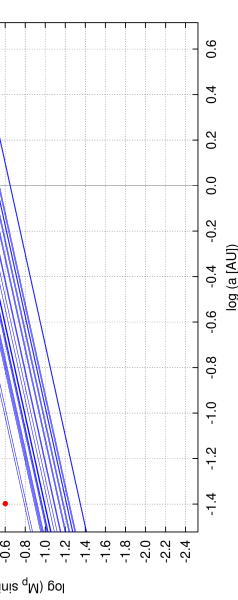
Figure 1.: Red dots: Masses and semi-major axes of currently known extrasolar planets. Blue lines: Upper (mass) and lower (orbital radius) limits for stars from the Lick survey (Cumming et al.1999).

2. Observations

The spectra were obtained at the 2.1m telescope of the McDonald Observatory with the Sandiford Echelle spectrograph. They cover a wavelength range from about 4840 to 7000 Å with a resolution of 60000. The list of the observed stars can be found in Tables 1 and 2. The reductions were done with IRAF (echelle order extraction) and a Windows based graphical package (ASP) for continuum and wavelength setting and equivalent width determination developed by REL. A comparison of equivalent widths with published values indicates agreement at the 5% level.

Table 1.: Observations of CGP dwarfs.

HD	date
8574	2001-08-23
	2001-08-27
9826	1999-10-19
	1999-10-23
10697	1992-11-03
	1992-11-05
	1992-11-07
	1997-02-03
	1999-10-19
12661	2000-08-18
	2000-08-21
19994	2000-10-20
	2001-02-11
	2001-08-23
	2001-08-25
28185	2001-10-25
	2001-10-27
33636	2002-01-23
	2002-01-26
37124	2000-01-26
	2000-01-29
38529	1992-11-04
	1992-11-05
	1992-11-07
	1993-03-10
	1997-01-31
	1997-02-02
50554	2001-10-23
	2001-10-27
52265	2001-10-24
	2001-10-27
68988	2002-01-24
	2002-01-26
74156	2001-10-25
	2001-10-28
75732	1993-03-03
	1993-03-05
	1993-03-11
	1993-03-07

HD	date
	1997-02-03
	1999-10-19
80606	2002-01-23
	2002-01-28
82943	2002-01-22
	2002-01-25
92788	2001-05-08
	2001-05-14
89744	2001-05-08
	2001-05-14
106252	2001-05-08
	2001-05-14
114762	1999-05-26
	1999-05-28
	2000-01-25
117176	1999-05-25
	1999-05-28
	2000-01-25
120136	1999-05-25
	1999-05-28
	2000-01-25
130322	2000-01-26
	2000-01-30
134987	2000-04-25
	2000-04-30
136118	2002-05-21
	2002-05-24
141937	2001-05-08
	2002-01-26
143761	1999-05-26
	1999-05-28
	2001-05-10
145675	1993-03-06
	1993-03-09
	1993-03-11
	1997-04-24
	1998-05-15
168443	1999-05-30
	1999-10-25

HD	date
169830	2000-08-18
	2000-08-21
177830	2000-08-18
	2000-08-21
178911	2001-05-08
	2001-05-14
	2001-08-27
179949	2001-08-24
	2001-08-28
186427	1999-05-26
	1999-05-28
	2000-08-19
187123	1999-05-30
	1999-10-25
190228	2000-10-22
	2001-08-23
	2001-08-27
192263	2000-08-19
	2000-08-21
195019	1999-05-30
	1999-10-25
209458	2000-08-18
	2000-08-21
210277	1999-10-19
	1999-10-25
217014	1992-11-03
	1992-11-06
	1992-11-07
	1997-10-18
	1999-10-19
217107	1999-10-19
	1999-10-24
222582	2000-08-18
	2000-08-21
BD -10 3166	2001-05-10
	2002-01-26
	2002-01-28
Callisto	2001-10-26
	2001-10-28

Table 2.: Observations of no-CGP dwarfs.

HD	date
166	1999-10-25
	2000-08-22
4628	1999-10-25
	2000-08-20
	2000-08-22
10476	2000-08-20
	2001-08-23
12235	1992-11-04
	1992-11-06
	1992-11-08
	1992-11-09
	1997-02-03
	1999-10-19
16160	2000-08-18
	2001-08-25
16895	2000-08-19
	2001-10-23
22484	1999-10-21
	1999-10-24
26965	1999-10-19
	1999-10-23

HD	date
32147	1992-11-03
	1992-11-05
	1992-11-08
	1993-03-10
	1995-10-11
	1997-01-31
	1997-02-02
48682	2000-10-20
	2001-10-25
	2001-10-27
50281	2001-10-26
	2002-01-25
76151	1993-03-04
	1993-03-06
	1993-03-07
	1993-03-10
	1997-02-03
	2000-01-29
84737	2002-05-21
	2002-05-24
126053	2002-05-21
	2002-05-24

HD	date
149661	1993-03-03
	1993-03-05
	1993-03-07
	1993-03-10
	1997-04-24
	1997-04-28
157214	2000-04-25
	2000-04-29
170657	2001-08-24
	2001-08-27
166620	2000-10-19
	2001-08-25
	2001-08-27
185144	1999-10-19
	1999-10-23
186408	1999-05-26
	1999-05-28
	2000-08-19
201091	1997-08-17
	1999-10-19
219134	1999-10-19
	1999-10-24
222368	2000-08-19
	2000-08-21

3. Analysis

The abundance analysis was done strictly differentially with respect to the Sun using a large sample of lines (cf. Figures 4a,b). We have obtained a solar flux spectrum (Callisto) using the same instrumentation and reduction procedure as used for our program stars. Figure 2 shows a portion of the observed spectra of HD 195019 and the Sun, as well as a synthetic spectrum, computed with SYNTH (Piskunov 1992). Synthetic equivalent widths were calculated and fit to the observations by variation of abundance for each line with the program LINES (originally by Sneden 1974). We used MARCS model atmospheres (Gustafsson et al. 1975) and an atomic data list compiled by REL. The relative abundance for each line was then calculated by subtracting the abundance obtained from the Callisto spectrum for the corresponding line. From all Fe lines available within the observed spectral range, only those giving an abundance within two standard deviations (2$\sigma$) from the mean have been retained for the derivation of the atmospheric parameters described in the following subsection. This was done in order to discard “outliers” automatically. For the calculation of the final mean abundances, however, the line list has been further reduced by rejecting all lines with an abundance deviation from the mean of more than 1$\sigma$, which decreased the errors of the abundances significantly.

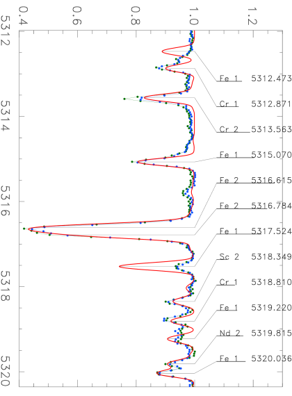
Figure 2.: Sample spectra of HD 195019 (green dots) and the Sun (Callisto, blue dots). Red line: synthetic spectrum. Note that for the Fe I line at 5317 Å the $gf$ value is obviously wrong, but this source of error is canceled out in a strictly differential analysis.

3.1. Atmospheric parameters

To determine the atmospheric parameters, iron line abundances were calculated for each star for a small ($T_{\rm eff}$, $\log g$, $v_{\rm micro}$) – grid, centered on $v_{\rm micro}$ = 1 km s^-1 and ($T_{\rm eff}$, $\log g$) determined by one of three methods in the following order of preference:

1. Literature data (previous abundance analyses)

2. Calibration for Geneva photometry (Künzli et al. 1997)

3. A new calibration for line-depth ratios and $T_{\rm eff}$ for our sample of dwarf stars. We used 20 of the 32 line-pairs which Kovtyukh and Gorlova (2000) had used for a similar calibration for supergiants, our observations, and effective temperatures from methods 1 and 2. An example for a useful (left panel) and a rejected (right panel) line-pair is shown in Figure 3. The line-ratio – $T_{\rm eff}$ relations were obtained from polynomial fits to the data, or calculated from synthetic spectra in some cases where only few datapoints were available.

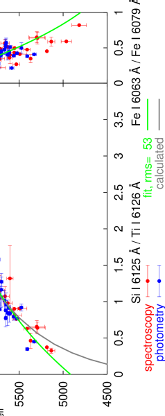
Figure 3.: Two examples for the dependence of line-depth ratios on effective temperature. Red: literature data, blue: Geneva photometry, green: polynomial fit, gray: relation for ratios calculated from synthetic spectra. The relation shown in the right panel has not been used for the calibration.

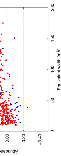
Figure 4.: Fe abundances in dex (0.00…[Fe]${}_{\hbox{$\odot$}}$) versus atomic data for HR 5072 and ($T_{\rm eff}$, $\log g$, $v_{\rm micro}$) = (5700, 4.0, 0.7). These parameters obviously do not correspond to the best-fit values.

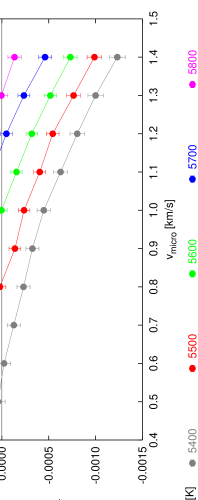
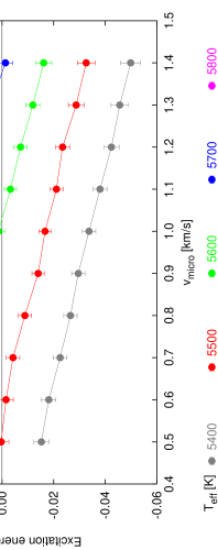
Figure 5.: Dependence of the slopes appearing in diagrams like those shown in Figure 4 on $v_{\rm micro}$ and $T_{\rm eff}$, for Fe I, here for $\log g$=4.1 (HR 5072). The errorbars are determined from linear regression.

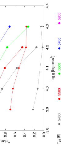
Figure 6.: Values of $v_{\rm micro}$, for which the slopes in the abundance versus atomic data diagrams vanish, in dependence of $T_{\rm eff}$ and $\log g$. Dots and diamonds correspond to equivalent width and excitation energy, respectively.

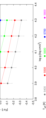
Figure 7.: Difference between the mean abundances of neutral and ionized iron, for $v_{\rm micro}$=1.0 km s^-1.The errorbars correspond to the standard deviation of the line abundances.

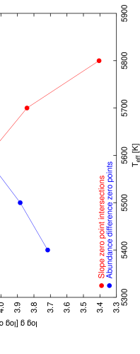
Figure 8.: Red: Intersections of two lines from Figure 6 corresponding to equivalent width and excitation energy. Blue: Combinations of $T_{\rm eff}$ and $\log g$, for which the difference between the mean abundances of neutral and ionized iron is zero (determined from Figure 7).

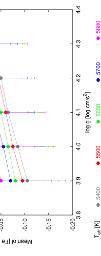
Figure 9.: Variation of the mean iron abundance with parameters. Here, the error bars indicate the abundance range covered by using the $v_{\rm micro}$ range of Figure 5.

The final atmospheric parameters were determined by driving the slopes of the line-strength and excitation energy relations with Fe I line abundance to zero and demanding ionization equilibrium. As an example, Figure 4 shows the trends visible in an abundance versus equivalent width or excitation energy diagram, if $T_{\rm eff}$, $\log g$, and $v_{\rm micro}$ deviate from the best-fit values by 100 K, 0.1 [cgs], and 0.3 km s^-1, respectively (for the planet host HR 5072). We determine the best-fit values by first identifying the value of $v_{\rm micro}$, for which the trends in the above mentioned diagrams are zero, for each model in the ($T_{\rm eff}$, $\log g$) grid (cf. Figure 5). Figure 6 shows these “zero-points” for equivalent width (dots) and excitation energy (diamonds) for each grid point. From the set of ($T_{\rm eff}$, $\log g$) models for which the two zero-points are equal (i.e. the intersections of two corresponding lines in Figure 6), we can finally identify one parameter pair, which gives the same abundance for neutral and ionized Fe lines. Figure 7 illustrates the dependence of the abundance difference [Fe I]$-$[Fe II] on $T_{\rm eff}$ and $\log g$. The dependence of this quantity on $v_{\rm micro}$ is negligible. The combination of information extracted from Figures 6 and 7 is shown in Figure 8. Figure 9 shows the variation of the mean Fe abundance within the parameter grid. From these diagrams we estimate the errors in our final spectroscopically determined parameters to be 50 K, 0.05 [cgs] and 0.05 km s^-1, for $T_{\rm eff}$, $\log g$, and $v_{\rm micro}$, respectively.

4. Results

4.1. Atmospheric parameters

A comparison of the parameters derived as described above with parameters found in the literature and derived from photometry results in the mean differences and standard deviations listed in Table 3 (parameter[this work] $-$ parameter[comparison]).

Table 3.: Differences between parameters determined in this work, in the literature and with photometric calibrations.

	N	$T_{\rm eff}$		$\log g$	[Fe]
Spectroscopy1	52∗	55 $\pm$	90	0.05 $\pm$ 0.20	0.02 $\pm$ 0.07
CGP dwarfs	37	50 $\pm$	90	0.05 $\pm$ 0.20	0.02 $\pm$ 0.08
No-CGP dwarfs	9	80 $\pm$	120	0.10 $\pm$ 0.20	0.02 $\pm$ 0.07
Geneva photometry2,3	41∗	45 $\pm$	75	0.00 $\pm$ 0.35	0.10 $\pm$ 0.09
Strömgren photometry3,4	50∗	190 $\pm$	110	0.25 $\pm$ 0.70	$-$0.10 $\pm$ 0.66

Table 4.: Parameters and Fe abundances for CGP dwarfs.

HD	$T_{\rm eff}$	$\log g$	$v_{\rm micro}$	[Fe]
8574	6100	4.30	1.45	$-$0.04$\pm$	0.05
9826	6200	4.40	1.60	0.13$\pm$	0.07
10697	5650	4.05	0.90	0.16$\pm$	0.06
12661	5700	4.10	0.50	0.39$\pm$	0.07
19994	6150	4.30	1.50	0.23$\pm$	0.07
28185	5700	4.20	0.80	0.24$\pm$	0.06
33636	6050	4.55	1.25	$-$0.11$\pm$	0.05
37124	5700	4.50	1.10	$-$0.38$\pm$	0.05
38529	5750	4.05	1.50	0.48$\pm$	0.12
50554	6050	4.50	1.20	$-$0.04$\pm$	0.04
52265	6100	4.40	1.30	0.15$\pm$	0.05
68988	6000	4.45	1.35	0.36$\pm$	0.06
74156	6050	4.35	1.25	0.09$\pm$	0.05
75732	5500	4.40	1.00	0.55$\pm$	0.16
80606	5700	4.40	0.90	0.46$\pm$	0.07
82943	5900	4.40	0.75	0.24$\pm$	0.04
89744	6300	4.40	1.80	0.22$\pm$	0.08
92788	5700	4.20	0.50	0.30$\pm$	0.06
106252	5890	4.40	1.10	$-$0.10$\pm$	0.04
114762	6000	4.40	1.50	$-$0.78$\pm$	0.06
117176	5600	4.10	1.00	$-$0.05$\pm$	0.03
120136	6600	4.70	1.90	0.37$\pm$	0.12
130322	5400	4.40	0.00	0.10$\pm$	0.06
134987	5720	4.25	0.70	0.35$\pm$	0.11
136118	6250	4.45	1.60	$-$0.03$\pm$	0.07
141937	5900	4.45	0.90	0.12$\pm$	0.04
143761	5900	4.40	1.25	$-$0.25$\pm$	0.04
145675	5500	4.30	1.10	0.59$\pm$	0.15
168443	5600	4.10	0.80	0.09$\pm$	0.04
169830	6300	4.40	1.60	0.09$\pm$	0.06
177830	5000	3.70	0.90	0.61$\pm$	0.14
178911	6050	4.50	1.10	0.15$\pm$	0.06
179949	6200	4.50	1.20	0.20$\pm$	0.06
186427	5800	4.40	0.95	0.06$\pm$	0.03
187123	5800	4.35	0.90	0.08$\pm$	0.04
190228	5360	3.90	0.90	$-$0.17$\pm$	0.04
192263	5100	4.45	0.00	0.11$\pm$	0.10
195019	5830	4.30	1.05	0.05$\pm$	0.04
209458	6100	4.50	1.30	$-$0.02$\pm$	0.05
210277	5700	4.40	1.20	0.27$\pm$	0.06
217014	5750	4.25	0.70	0.24$\pm$	0.05
217107	5750	4.35	1.15	0.39$\pm$	0.06
222582	5800	4.40	0.80	0.03$\pm$	0.04
BD $-$10 3166	5550	4.45	1.00	0.51$\pm$	0.10

Table 5.: Parameters and Fe abundances for no-CGP dwarfs.

HD	$T_{\rm eff}$	$\log g$	$v_{\rm micro}$	[Fe]
166	5550	4.50	0.80	0.13$\pm$	0.05
4628	5150	4.60	0.80	$-$0.21$\pm$	0.08
10476	5200	4.35	0.00	0.03$\pm$	0.07
12235	6100	4.40	1.60	0.35$\pm$	0.11
16160	5100	4.55	0.60	$-$0.03$\pm$	0.14
16895	6500	4.70	1.70	0.07$\pm$	0.08
22484	6050	4.30	1.55	$-$0.07$\pm$	0.09
26965	5300	4.55	0.70	$-$0.26$\pm$	0.08
32147	5400	4.65	1.95	0.50$\pm$	0.30
48682	6200	4.60	1.30	0.13$\pm$	0.13
50281	5100	4.50	1.40	0.00$\pm$	0.13
76151	5700	4.35	0.65	0.10$\pm$	0.05
84737	5950	4.30	1.30	0.07$\pm$	0.04
126053	5650	4.40	0.65	$-$0.44$\pm$	0.04
149661	5300	4.40	0.00	0.15$\pm$	0.13
157214	5650	4.35	0.60	$-$0.44$\pm$	0.06
166620	5200	4.50	0.50	$-$0.09$\pm$	0.10
170657	5200	4.55	0.60	$-$0.11$\pm$	0.08
185144	5400	4.50	1.00	$-$0.20$\pm$	0.06
186408	5780	4.35	0.85	0.09$\pm$	0.04
201091	5200	4.50	2.00	$-$0.22$\pm$	0.21
219134	5100	4.40	0.90	0.10$\pm$	0.13
222368	6300	4.40	1.70	$-$0.11$\pm$	0.07

4.2. Fe abundances

The parameters and Fe abundances determined spectroscopically in this work are given in Tables 4 and 5. Figure 10 shows the Fe abundances as a function of effective temperature for the two different groups of stars. For the calculation of the model atmospheres we used ODFs with solar abundances scaled according to the derived Fe abundances. We found this to be particularly important for overabundant stars, for which the abundances were underestimated when ODFs with solar abundances were used.

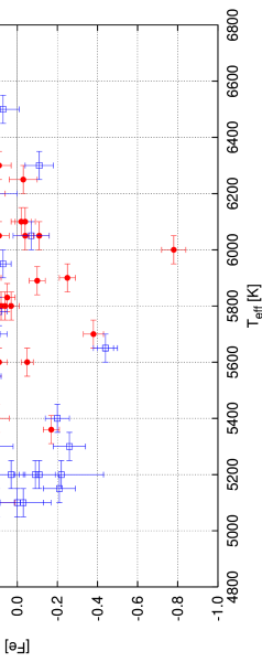
Figure 10.: Fe-abundances (relative to the Sun) of CGP and no-CGP dwarfs.

5. Conclusions

At this point of time we cannot draw any hard conclusions, because

• the sample sizes are limited;

• the analysis is still incomplete;

• the samples could be affected by selection bias.

However, Figure 10 indicates that

• in contrast to the no-CGP sample, there seems to be a lack of cool stars ($T_{\rm eff}\leq$ 5400 K) in the CGP sample. Does this mean a bias in the sample selection?

• there is a “clump” of metal-rich CGP stars at solar temperature. Is this a lack of metal poor giant planet hosts or a bias – either from selection or from a lack of metal poor solar type stars (with or without planets)?

• there seems to be no correlation between metallicity and planet hosting at hotter temperatures ($T_{\rm eff}\geq$ 6000 K).

Planned future work includes:

• Abundance analysis of a second comparison sample: Stars which have spectral types like those of the dwarfs with (CG) planets selected randomly from the Bright Star Catalog (and Supplement);

• Abundance analysis of “Very Strong Lined” dwarfs (Eggen 1978);

• Abundance determination for elements other than Fe, for all stars of the four samples.

Acknowledgments.

This research has been supported by a grant from the National Science Foundation (NSF). Use was made of the Simbad database, operated at CDS, Strasbourg, France.

References

Cumming, A., Marcy, G. W., & Butler, R. P. 1999, ApJ 526, 890

Edvardsson, B., Andersen, J., Gustafsson, B., Lambert, D. L., Nissen, P. E., & Tomkin, J. 1993, A&A 275, 101

Fuhrmann, K. 1998, A&A 338, 161

Gonzalez, G. 1997, MNRAS 285, 403

Gonzalez, G. 1998, A&A 334, 221

Gonzalez, G., & Vanture, A. D. 1998, A&A 339, L29

Gonzalez, G., Wallerstein, G., & Saar, S. H. 1999, ApJ 511, L.111

Gonzalez, G., & Laws, C. 2000, AJ 119, 390

Gonzalez, G., Laws, C., Tyagi S., & Reddy B. E. 2001, AJ 121,432

Gustafsson, B., Bell, R. A., Eriksson, K., & Nordlund, A. 1975, A&A 42, 407

Kovtyukh, V. V., & Gorlova, N. I. 2000, A&A 358, 587

Künzli, M., North, P., Kurucz, R. L., & Nicolet, B. 1997, A&AS 122, 51

Mermilliod, J.-C., Mermilliod, M., & Hauck, B. 1997, A&AS 124, 349

Napiwotzki, R., Schönberner, D., & Wenske, V. 1993, A&A 268, 653

Piskunov, N. E., 1992, in “Stellar magnetism”, Nauka, St. Petersburg, p. 92

Santos, N. C., Israelian, G., & Mayor, M. 2000, A&A 363, 228

Santos, N. C., Israelian, G., & Mayor, M. 2001a, A&A 373, 1019

Santos, N. C., Israelian, G., & Mayor, M. 2001b, Proc. 12th Cambridge workshop “Cool Stars, Stellar Systems, and the Sun”, in press

Sneden, C. A. 1974, PhD Thesis, The University of Texas at Austin