Abstract

As a special contribution to the proceedings of the BeppoSAX workshop dedicated to blazar astrophysics we present a catalog of 157 X-ray spectra and the broad-band Spectral Energy Distribution (SED) of 84 blazars observed by BeppoSAX during its first five years of operations. The SEDs have been built by combining BeppoSAX LECS, MECS and PDS data with (mostly) non-simultaneous multi-frequency photometric data, obtained from NED and from other large databases, including the GSC2 and the 2MASS surveys. All BeppoSAX data have been taken from the public archive and have been analysed in a uniform way. For each source we present a $\nu f(\nu)~{}vs~{}\nu$ plot, and for every BeppoSAX observation we give the best fit parameters of the spectral model that best describes the data. The energy where the maximum of the synchrotron power is emitted spans at least six orders of magnitudes ranging from $\approx 0.1~{}$eV to over $100~{}$keV. A wide variety of X-ray spectral slopes have been seen depending on whether the synchrotron or inverse Compton component, or both, are present in the X-ray band. The wide energy bandpass of BeppoSAX allowed us to detect, and measure with good accuracy, continuous spectral curvature in many objects whose synchrotron radiation extends to the X-ray band. This convex curvature, which is described by a logarithmic parabola law better than other models, may be the spectral signature of a particle acceleration process that becomes less and less efficient as the particles energy increases. Finally some brief considerations about other statistical properties of the sample are presented.

1 Introduction

Blazars emission is known to be dominated by strong and highly variable non-thermal radiation across the entire electromagnetic spectrum. Multi-frequency ground based observations, combined with data from high energy astronomy satellites, have often been used to derive the broad-band Spectral Energy Distribution (SED) of blazars, that is the source intensity as a function of energy, usually represented in the $\nu f(\nu)~{}vs~{}\nu$ or $\nu L(\nu)~{}vs~{}\nu$ space. These measurements are consistent with the widely accepted scenario where blazar emission is due to synchrotron radiation whose power increases with energy up to a peak value above which it drops sharply. At higher energies the spectrum is dominated by inverse Compton emission which also smoothly raises until it reaches a second luminosity peak. The often extreme observational characteristics of blazars are thought to be the result of the emission from a relativistic jet seen at a very small angle with respect to the line of sight (e.g. Urry & Padovani 1995), an interpretation first proposed by Blandford & Rees (1978). According to this scenario the position and the relative power of the synchrotron and inverse Compton peaks directly depend on important physical parameters such as the intensity of the magnetic field, the maximum energy at which electrons can be accelerated, and the relativistic motion and orientation of the emitting plasma. The synchrotron peak is located at energies ranging from less than $\approx 0.1~{}$eV (or $\nu\approx 10^{13}~{}$Hz) to well over $10~{}$keV (or $\nu\approx 10^{18}~{}$Hz) or even 100 keV in flaring states, demonstrating the existence of a wide variety of physical and geometric conditions in blazars. For these reasons the Spectral Energy Distribution of blazars has been and still is the subject of intense research activity. Figure 1 shows the expected emission from Synchrotron Self Compton models (SSC) tracing a hypothetical sequence of blazar SEDs that ranges from LBL sources where the synchrotron peak frequency ($\nu_{peak}$ ) occurs at low energies to HBL objects where $\nu_{peak}$ reaches the X-ray band, and up to the extremely large $\nu_{peak}$ energies of the, possibly existing but still unseen, Ultra High energy peaked BL Lacs (UHBLs). As shown in Figure 1, within the broad-band energy spectrum of blazars the X-ray region is particularly important since at these energies a variety of different spectral components can be (and have been) seen. These include the flat and rising Compton component, the transition between the two regimes, and the high energy end of the synchrotron spectrum which is produced by very, sometimes extremely, energetic electrons. These crucial observations, in combination with other multi-frequency data allow the determination of the overall spectral shape and therefore the estimation of important physical parameters.

With its very wide X-ray band pass, good sensitivity and spectral capabilities BeppoSAX has provided a very important opportunity to study blazars astrophysics, especially when simultaneous multi-frequency observations could be arranged.

As a special contribution to the proceedings of the BeppoSAX workshop dedicated to blazar Astrophysics we present the catalog of X-ray spectral fits and broad-band Spectral Energy Distribution of all the blazars observed with BeppoSAX whose data are currently public.

Fig. 1.: The Spectral Energy Distribution of BL Lacs is shown as a sequence of Synchrotron Self Compton spectra peaking at different energies. Objects whose synchrotron component peaks at low energy are called LBLs, the maximum of their synchrotron power output occurs in the IR-Optical band, while High energy peaked BL Lacs (HBLs) peak in the UV or X-ray band. It is not known how far the sequence of $\nu_{peak}$ goes on. If it continues to very high energies it could be that in some very extreme objects (UHBLs) the synchrotron component might even reach the gamma-ray band. Note that for the same peak luminosity, the radio power decreases by orders of magnitudes in going form LBLs to HBLs and possibly to UHBLs.

2 BeppoSAX Blazars: the sample

A complete description of the BeppoSAX X-ray astronomy satellite is given in Boella et al. (1997a). The scientific instrumentation is composed of six co-aligned Narrow Field Instruments (NFI) and two Wide Field Cameras (WFC, Jager et al. 1997) pointing in opposite directions and perpendicularly to the pointing direction of the NFI. The NFI include the Low Energy Concentrator Spectrometer, (LECS, Parmar et. al 1997), three identical Medium Energy Concentrator Spectrometers, (MECS, Boella et al. 1997b), one of which (MECS1) failed in May 1997, a High Pressure Gas Scintillation Proportional Counter (HPGSPC, Manzo et al. 1997), and a Phoswich Detector System (PDS, Frontera et al. 1997). Collectively the NFI cover a very wide spectral range (0.1–200 keV) providing an unprecedented opportunity to study the broad band SED of blazars. During its lifetime BeppoSAX dedicated approximately 15% of its scientific program to the study of blazars performing about 200 observations of nearly 100 blazars.

We have carried out a systematic analysis of all blazar observations made with the LECS, MECS and PDS (for sufficiently bright and unconfused sources) instruments and for which the corresponding data were available in the BeppoSAX public archive (Giommi & Fiore 1997) at the date of March 2002. As BeppoSAX data are subject to the usual one year proprietary period, this approximately corresponds to observations performed in the period July 1996 - March 2001. The blazar class is usually divided in BL Lacs and Flat Spectrum Radio Quasars (FSRQs), these last also including GigaHertz Peaked Spectrum (GPS) QSOs.

Our list includes a total of 84 blazars, 58 of which are BL Lacs, 22 are FSRQs, and 4 (1JY 2149$-$3006, PKS 2126$-$15, OX 57 and PKS 2243$-$123) are GPS QSOs. These sources were observed as part of several BeppoSAX projects and were discovered both in the radio and the X-ray band, sometimes in surveys with widely different flux limits. In addition the BeppoSAX selection process clearly favoured objects that were known to be X-ray bright and possibly detectable by the high energy instruments (PDS). The sample is therefore highly heterogeneous and cannot be used for detailed statistical analyses requiring strict completeness criteria. The size of the sample and its heterogeneity nevertheless provide an unprecedented opportunity to explore a very wide portion of the blazar parameter space.

The lists of BL Lacs and FSRQs considered in this paper are presented in Tables I and II, respectively. Column 1 gives the name of the object, columns 2 and 3 give the Right Ascension and Declination for the equinox 2000.0, column 4 gives the redshift when available, column 5 gives the number of BeppoSAX observations available in the public archive, and column 6 gives the references to previous BeppoSAX publications.

In general, sources brighter than $\approx 5\times 10^{-12}~{}$ erg cm${}^{-2}~{}$s${}^{-1}~{}$can be detected in all three BeppoSAX NFI instruments considered in this paper (LECS, MECS, and PDS), fainter sources can only be detected in the imaging instruments (LECS and MECS) up to 10 keV. A total of 157 spectra have been analysed.

3 Data analysis

All LECS, MECS and PDS cleaned and calibrated spectral data (pha files) have been taken from the BeppoSAX public archive (Giommi & Fiore 1997). The standard BeppoSAX procedure that generated these archival spectra used photons located within a circular region centered on the source with a typical radius of 4 arcminutes for the MECS data and of 6 arcminutes for the LECS data. For the case of weak sources, however, this procedure used a radius of 4 and sometimes even 2 arcminutes to extract the LECS spectra, a value that turned out to be too small to ensure a good signal-to-noise ratio. All LECS spectral files that were originally produced using a 2 arcminutes radius have been re-generated by us using a more adequate 4 arcminutes radius. In a few cases non-standard extraction radii had to be used to avoid contamination from a nearby source. Background subtraction was carried out using the standard background files available from the BeppoSAX archive. Since these background data were taken observing “blank” areas of the sky (that is fields not including a detectable target) with low Galactic absorption ($N_{H}$), the low energy counts of X-ray sources located in regions of high $N_{H}$ may be underestimated. We have therefore ignored data below 0.3 keV. Finally, spectral channels were binned in such a way that each channel includes at least 20 counts.

All data were analysed in a homogeneous way following the recommendations given in the BeppoSAX handbook for NFI spectral analysis (Fiore et al. 1999).

We have combined LECS data covering the range 0.3–2.0 keV, MECS data between 2–10 keV, and, for bright and unconfused sources, PDS data above 12 keV and up to the maximum energy at which these sources could be detected.

3.1 Spectral models

Spectral fits have been done with the XSPEC 11.0 package using one of the following spectral models

1. single power law

   $dN/dE=ke^{-\sigma(E)N_{H}}E^{-\gamma}$

2. sum of two power laws

   $dN/dE=e^{-\sigma(E)N_{H}}(kE^{-\gamma}+k_{1}E^{-\gamma_{1}})$

3. broken power law

   $dN/dE=\left\{\begin{array}[]{ll}ke^{-\sigma(E)N_{H}}E^{-\gamma}\quad\quad\quad\,\,\,\,\,\,\,\mbox{if}\quad E<E_{break}\\[5.69046pt] kE_{break}^{\gamma_{1}-\gamma}e^{-\sigma(E)N_{H}}E^{-\gamma_{1}}\quad\mbox{if}\quad E\geq E_{break}\end{array}\right.$

4. logarithmic parabola

   $dN/dE=ke^{-\sigma(E)N_{H}}E^{(-\gamma+\beta Log(E))}$

in this last case $\gamma$ is the photon spectral index at 1 keV and $\beta$ is the coefficient of the quadratic term in the logarithmic parabola ($Log(dN/dE)=log(k)-\gamma Log(E)+\beta(Log(E))^{2}$), which is proportional to the slope change in an energy decade. This spectral law was first used by Landau et al. (1986) who were able to obtain very good fits to the wide band spectra (mm to optical-UV) of a number of BL Lacs. More recently, Massaro et al. (2000) and Cusumano et al. (2001) successfully applied this model to fit the X-ray spectra of young pulsars and developed the XSPEC routine used in the present work. With respect to other curved spectra, the log-parabola has the advantage of describing well the spectral curvature that is often seen in the broad band spectrum of blazars with only three parameters. Furthermore, as discussed by Massaro (2002), it is possible to show that a log-parabolic spectrum is naturally obtained by a statistical acceleration mechanism where the probability for a particle to remain inside the acceleration region is assumed to decrease as the particles energy grows.

The amount of $N_{H}$ in the low energy absorption term ($e^{-\sigma(E)N_{H}}$) was always fixed to the Galactic value as estimated from the 21 cm measurements of Dickey & Lockman (1990).

The LECS-MECS and MECS-PDS relative normalizations were treated as free parameters but constrained to be within 0.6 and 1.1 and 0.8-1.0, respectively. Typical values are 0.7 for LECS/MECS and 0.9 for MECS/PDS, as expected from the BeppoSAX NFI intercalibration (see Fiore et al. 1999 for details).

3.2 Results of the spectral fitting

The results of our spectral fits are reported in Tables III-IV, where, for each source, we give the best fit parameters for the spectral model that gives the lowest $\chi^{2}$. For sources that were observed more than once only one model was used choosing the one that gives the lowest $\chi^{2}$ in most of the observations.

Column 1 gives the source name built with the J2000.0 coordinates (for reasons of space we use here a IAU like naming convention rather than the full name), column 2 gives the observation date, columns 3, 4, 5, 6 and 7 give the model used and the best fit parameters (with one sigma errors), column 8 gives the reduced $\chi^{2}$ and the number of degrees of freedom, column 9 gives the 2–10 keV flux in units of erg cm${}^{-2}~{}$s${}^{-1}~{}$.

To keep the amount of work manageable we have neglected the effects of rapid variability always integrating the spectral data over the full observation. The high $\chi^{2}$ values that resulted from the analysis of some rapidly variable sources are due to significant spectral changes that usually accompany large intesity variations (e.g. Giommi et al. 1990, Tanihata et al. 2001). The best estimates of the $\beta$ parameter in model 4 are mostly negative and between $-$0.5 and $-$0.15; the few positive values attest the presence of an upward spectral curvature due to presence of both the synchrotron and the Compton component in the BeppoSAX band.

As all of the data used in this work are publicly available, a large fraction of the BeppoSAX spectra has already been analysed and published by the original investigators. We have therefore compared the results of our fits with published results and we have found that, when the spectral model used is the same, our best fit parameters agree well with the published values.

3.3 Spectral Energy Distributions

In order to build the broad band (radio to hard X-ray) Spectral Energy Distributions we have first converted all BeppoSAX spectra into flux using the best model and best fit parameters listed in Tables III-IV. We have then de-reddened the soft X-ray fluxes using the cross sections of Morrison & McCammon (1983) setting the amount of absorbing material ($N_{H}$) equal to the Galactic value, consistently with the fitting procedure. We have then combined these X-ray fluxes with (mostly non-simultaneous) multi-frequency photometric measurements available from NED or from specific BeppoSAX publications. We have also added infrared and optical fluxes converting magnitudes from the blazars counterparts in the 2MASS and GSC2 catalogs (when available) using the prescriptions given in Cardelli et al. (1989). In several nearby objects (e.g. Mkn 421, Mkn 501, 3C 66A, PKS 0548$-$322) the optical emission is dominated by the host galaxy and therefore our fluxes should be considered as an upper limit to the non-thermal nuclear emission.

All SEDs are plotted in Figures 2a through 2o for BL Lacs and in Figures 3a through 3g for FSRQs. Fluxes have not been corrected for redshift and therefore are in the observer’s frame.

All the SEDs, including the data files, and spectral fitting details are also available on-line from the ASI Science Data Center web server at the following address

http://www.asdc.asi.it/blazars/

TABLE I
: BL Lacs available in the BeppoSAX public archive

Blazar name	Ra(J2000.0)	Dec(J2000.0)	Redshift	No. of	Ref.
				observ.
1ES 0033+595	00 35 52.7	59 50 03.8	$-$	1	a
PKS 0048$-$097	00 50 41.3	$-$09 29 04.9	$-$	2	b
1ES 0120+340	01 23 08.6	34 20 48.8	0.272	2	a
RGB J0136+39	01 36 32.7	39 06 00.0	$-$	1
1ES 0145+138	01 48 29.7	14 02 17.8	0.125	1	c
MS 0158.5+0019	02 01 06.1	00 34 00.1	0.299	1	d
3C 66A	02 22 39.6	43 02 08.1	0.444	2
AO 0235+164	02 38 38.8	16 36 59.0	0.94	1	e
MS 0317.0+1834	03 19 51.9	18 45 33.8	0.19	1	d
1H 0323+022	03 26 13.8	02 25 14.8	0.147	1	c
1ES 0347$-$121	03 49 23.2	$-$11 59 26.8	0.188	1	d
1H 0414+009	04 16 52.3	01 05 24.0	0.287	1	d
1ES 0502+675	05 07 56.2	67 37 23.8	$0.314$	1	d
1H 0506$-$039	05 09 38.0	$-$04 00 46.0	0.304	1	c
PKS 0521$-$365	05 22 57.7	$-$36 27 02.8	0.055	1	m
PKS 0537$-$441	05 38 50.3	$-$44 05 08.8	0.896	1	n
PKS 0548$-$322	05 50 41.9	$-$32 16 10.9	0.069	3	a
S5 0716+714	07 21 53.4	71 20 35.8	$-$	3	g
MS 0737.9+7441	07 44 05.4	74 33 57.9	0.315	1	d
OJ 287	08 54 48.9	20 06 30.9	0.306	1	b,f
B2 0912+29	09 15 52.2	29 33 23.0	$-$	1	b
1ES 0927+500	09 30 37.6	49 50 26.1	0.188	1	c
1ES 1028+511	10 31 18.5	50 53 34.0	0.361	1	c
RGB J1037+57	10 37 44.3	57 11 54.9	$-$	1
RGB J1058+56	10 58 37.7	56 28 10.9	$-$	2
1H 1100$-$230	11 03 37.7	$-$23 29 30.8	0.186	2	d
Mkn 421	11 04 27.2	38 12 32.0	0.031	15	h,i,j
1RXS J111706.3+20141	11 17 06.3	20 14 09.9	0.137	1
EXO 1118.0+4228	11 20 48.0	42 12 11.8	0.124	1	c
Mkn 180	11 36 26.4	70 09 28.0	0.046	1	d
PKS 1144$-$379	11 47 01.3	$-$38 12 11.1	1.048	1	b
1RXS J121158.1+22423	12 11 58.0	22 42 36.0	0.77	3
EXO 1215.3+3022	12 17 52.1	30 07 00.1	0.237	2
1H 1219+301	12 21 22.0	30 10 36.8	0.13	1
ON 231	12 21 31.7	28 13 58.0	0.102	2	k
1RXS J123511.1$-$14033	12 35 11.1	$-$14 03 32.0	0.406	3
1ES 1255+244	12 57 31.8	24 12 39.9	0.141	1	c
MS 1312.1$-$4221	13 15 03.4	$-$42 36 50.0	0.105	1
EXO 1415.6+2557	14 17 56.2	25 43 55.9	0.237	3
PG 1418+546	14 19 46.6	54 23 15.0	0.152	3	e
1H 1430+423	14 28 32.4	42 40 23.8	0.13	1
MS 1458.8+2249	15 01 01.8	22 38 03.8	0.235	1	f
1H 1515+660	15 17 47.4	65 25 23.1	0.702	1	d
PKS 1519$-$273	15 22 37.6	$-$27 30 11.1	$-$	1
1ES 1533+535	15 35 00.7	53 20 36.9	0.89	1	c
1ES 1544+820	15 40 15.6	81 55 05.8	$-$	1	c
1ES 1553+113	15 55 43.1	11 11 21.1	0.36	1	c
Mkn 501	16 53 52.2	39 45 37.0	0.033	11	l

^a Costamante et al. 2001, ^b Padovani et al. 2001, ^c Beckmann et al. 2002, ^d Wolter et al. 1998, ^e Padovani et al. 2002a, ^f Massaro et al. 2002, ^g Giommi et al. 1999, ^h Fossati et al. 2000a,
ⁱ Fossati et al. 2000b, ^jMalizia et al. 2000, ^k Tagliaferri et al. 2000, ^lPian et al. 1998,
^mTavecchio et al. 2002, ⁿPian et al. 2002

TABLE I
: BL Lacs available in the BeppoSAX public archive - Continued

Blazar name	Ra(J2000.0)	Dec(J2000.0)	Redshift	No. of	Ref.
				observ.
1ES 1741+196	17 43 57.5	19 35 09.9	0.083	1	a
S5 1803+784	18 00 45.6	78 28 04.0	0.684	1	b
3C 371	18 06 50.7	69 49 27.8	0.051	1	b
S4 1823+568	18 24 07.1	56 51 01.0	0.664	1	c
1ES 1959+650	19 59 59.9	65 08 54.9	0.048	3	d
PKS 2005$-$489	20 09 25.3	$-$48 49 54.1	0.071	2	c
PKS 2155$-$304	21 58 51.9	$-$30 13 31.0	0.116	3	e,f,g
BL Lacertae	22 02 43.2	42 16 40.0	0.069	5	c,h
1ES 2344+514	23 47 04.7	51 42 17.9	0.044	7	i
1H 2354$-$315	23 59 07.8	$-$30 37 39.0	0.165	1

^a Siebert et al. 1999, ^b Padovani et al. 2002a, ^c Padovani et al. 2001, ^d Beckmann et al. 2002,
^e Giommi et al. 1998, ^f Chiappetti et al. 1999, ^g Zhang et al. 1999, ^h Ravasio et al. 2002,
ⁱ Giommi et al. 2000

TABLE II
: Flat Spectrum Radio Quasars available in the BeppoSAX public archive

Blazar name	Ra(J2000.0)	Dec(J2000.0)	Redshift	No. of	Ref.
				observ.
PKS 0208$-$512	02 10 46.1	$-$51 01 01.9	1.003	1	a
NRAO 140	03 36 30.0	32 18 29.8	1.259	1
PKS 0523$-$33	05 25 06.1	$-$33 43 05.0	4.401	1	b
OG 147	05 30 56.3	13 31 54.8	2.06	8	c
WGA J0546.6$-$6415	05 46 42.4	$-$64 15 21.9	0.323	1	d
1Jy 0836+710	08 41 24.4	70 53 40.9	2.19	1	e
RGB J0909+039	09 09 15.8	03 54 42.1	3.2	1	f
1Jy 1127$-$145	11 30 07.0	$-$14 49 27.1	1.187	1
3C 273	12 29 06.6	02 03 07.9	0.158	9	g
3C 279	12 56 11.1	$-$05 47 21.1	0.538	5	h
B3 1428+422	14 30 23.5	42 04 36.1	4.715	1	i
GB 1508+5714	15 10 02.8	57 02 47.0	4.301	2	f
PKS 1510$-$08	15 12 50.4	$-$09 05 59.9	0.361	1	e
1ES 1627+402	16 29 01.3	40 07 58.0	0.272	1	d
3C 345	16 42 58.7	39 48 36.0	0.594	1	a
V 396 HER	17 22 41.3	24 36 19.0	0.175	1	d
4C 62.29	17 46 13.9	62 26 53.8	3.886	1	f
S5 2116+81	21 14 01.6	82 04 46.9	0.086	2	d
PKS 2126$-$15	21 29 12.0	$-$15 38 41.9	3.266	1
OX 57	21 36 38.4	00 41 53.8	1.936	1
1Jy 2149$-$306	21 51 55.3	$-$30 27 53.9	2.34	1	j
PKS 2223+21	22 25 38.0	21 18 06.1	1.949	1	a,f
3C 446	22 25 47.2	$-$04 57 01.0	1.404	1
CTA 102	22 32 36.4	11 43 50.8	1.037	5	e
PKS 2243$-$123	22 46 18.1	$-$12 06 51.8	0.63	1	a
3C 454.3	22 53 57.6	16 08 53.1	0.86	1	a

^a Tavecchio et al. 2002, ^b Fabian et al. 2001a, ^c Ghisellini et al. 1999, ^d Padovani et al. 2002b,
^e Tavecchio et al. 2000, ^f Costantini et al. 1999, ^g Mineo et al. 2000, ^h Ballo et al. 2002,
ⁱ Fabian et al. 2001b, ^j Elvis et al. 2000

TABLE III
: Results of spectral fits for the sample of BL Lacertae Objects

Blazar name	Observ.	model(a)		Best fit parameters			$\chi^{2}/d.o.f.$	flux(b)
	date		$\gamma$	$\gamma_{1}$	$\beta$	$E_{break}$	(d.o.f.)
0035+5950	18-12-99	4	$1.42\pm 0.08$		$-0.44\pm 0.06$		0.95(85)	5.83
0050$-$0929	19-12-97	1	$1.9\pm 0.2$				0.52(9)	0.13
0123+3420	03-01-99	4	$1.8\pm 0.1$		$-0.2\pm 0.1$		1.1(45)	1.71
	02-02-99	4	$1.9\pm 0.2$		$-0.4\pm 0.2$		0.9(45)	1.31
0136+3906	09-01-01	4	$2.0\pm 0.1$		$-0.5\pm 0.1$		1.39(44)	1.05
0148+1402	30-12-97	1	$2.2\pm 0.4$				0.57(8)	0.05
0201+0034	16-08-96	4	$2.8\pm 0.3$		$0.5\pm 0.3$		1.21(22)	0.3
0222+4302	31-01-99	1	$2.2\pm 0.1$				0.75(24)	0.20
0238+1636	28-01-99	1	$1.9\pm 0.2$				0.9(22)	0.08
0319+1845	15-01-97	4	$1.5\pm 0.3$		$-0.5\pm 0.3$		0.74(39)	0.7
0326+0225	20-01-98	1	$2.2\pm 0.1$				1.3(22)	0.3
0349$-$1159	10-01-97	4	$1.8\pm 0.2$		$-0.4\pm 0.2$		0.92(42)	0.6
0416+0105	21-09-96	1	$2.6\pm 0.06$				0.75(34)	0.85
0507+6737	06-10-96	1	$2.31\pm 0.04$				1.34(37)	1.94
0509$-$0400	11-02-99	1	$2.00\pm 0.07$				1.20(37)	0.56
0522$-$3627	02-10-98	1	$1.75\pm 0.04$				0.83(54)	0.88
0538$-$4405	28-11-98	1	$1.75\pm 0.07$				0.68(42)	0.24
0550$-$3216	20-02-99	4	$1.53\pm 0.13$		$-0.49\pm 0.11$		0.96(56)	2.28
	07-04-99	4	$1.74\pm 0.15$		$-0.45\pm 0.14$		0.82(43)	1.52
0721+7120	14-11-96	3	$2.3\pm 0.1$	$1.8\pm 0.2$		$3.7\pm 0.6$	1.11(41)	0.14
	07-11-98	3	$2.1\pm 0.2$	$1.7\pm 0.2$		$2.9\pm 0.9$	1.46(36)	0.26
	30-10-00	3	$2.6\pm 0.1$	$1.7\pm 0.1$		$3.0\pm 0.3$	0.99(48)	0.33
0744+7433	29-10-96	1	$2.62\pm 0.15$				1.32(18)	0.15
0854+2006	24-11-97	1	$1.62\pm 0.12$				0.99(17)	0.21
0915+2933	14-11-97	1	$2.36\pm 0.09$				1.36(42)	0.26
0930+4950	25-11-98	4	$1.7\pm 0.1$		$-0.4\pm 0.1$		1.08(42)	0.67
1031+5053	01-05-97	1	$2.40\pm 0.05$				1.05(40)	1.03
1037+5711	02-12-98	1	$2.5\pm 0.1$				0.98(22)	0.09
1058+5628	21-05-98	1	$2.7\pm 0.3$				0.68(14)	0.03
	23-11-98	1	$2.8\pm 0.1$				0.91(16)	0.17
1103$-$2329	04-01-97	1	$2.07\pm 0.03$				1.10(242)	3.81
	19-06-98	1	$2.25\pm 0.02$				1.32(85)	2.56
1104+3812	29-04-97	4	$2.23\pm 0.03$		$-0.46\pm 0.03$		1.40(108)	8.5(c)
	30-04-97	4	$2.21\pm 0.03$		$-0.51\pm 0.03$		0.76(102)	8.3
	01-05-97	4	$2.19\pm 0.03$		$-0.47\pm 0.03$		1.03(102)	10.0
	02-05-97	4	$2.16\pm 0.04$		$-0.51\pm 0.04$		0.91(104)	12.3
	03-05-97	4	$2.24\pm 0.06$		$-0.52\pm 0.06$		0.98(89)	7.1
	04-05-97	4	$2.49\pm 0.07$		$-0.47\pm 0.07$		0.97(84)	4.1
	05-05-97	4	$2.29\pm 0.04$		$-0.54\pm 0.04$		1.17(88)	6.3
	21-04-98	4	$2.12\pm 0.01$		$-0.47\pm 0.01$		1.10(140)	17.8
	23-04-98	4	$1.99\pm 0.01$		$-0.43\pm 0.01$		1.50(136)	31.0(c)
	22-06-98	4	$2.03\pm 0.02$		$-0.39\pm 0.02$		1.27(123)	23.9
	04-05-99	4	$2.30\pm 0.01$		$-0.53\pm 0.01$		1.44(137)	11.1
	26-04-00	4	$1.75\pm 0.01$		$-0.26\pm 0.01$		2.72(130)	61.9(c)
	28-04-00	4	$1.72\pm 0.01$		$-0.26\pm 0.01$		1.67(130)	66.8(c)
	30-04-00	4	$1.72\pm 0.01$		$-0.32\pm 0.01$		1.72(130)	59.8(c)
	09-05-00	4	$1.82\pm 0.01$		$-0.23\pm 0.01$		3.05(130)	49.5(c)
1117+2014	13-12-99	4	$2.34\pm 0.09$		$-0.6\pm 0.1$		1.89(41)	0.61
1120+4212	01-05-97	1	$2.7\pm 0.1$				0.73(19)	0.29
1136+7009	10-12-96	4	$2.1\pm 0.2$		$-0.4\pm 0.2$		0.85(36)	0.51
1147$-$3812	10-01-97	1	$1.6\pm 0.2$				1.02(17)	0.09
1211+2242	27-12-99	4	$1.6\pm 0.3$		$-0.5\pm 0.3$		1.24(41)	0.24
1217+3007	23-12-98	2	$3.0\pm 2.1$	$1.0\pm 1.5$			1.09(17)	0.07
1221+3010	12-07-99	4	$2.21\pm 0.08$		$-0.31\pm 0.07$		0.83(88)	1.49
1221+2813	11-05-98	2	$2.8\pm 0.1$	$0.6\pm 0.3$			0.97(60)	0.42
	11-06-98	2	$2.9\pm 0.3$	$1.1\pm 0.4$			1.19(46)	0.33

^(a) 1: single power law, 2: double power law, 3: broken power law, 4: logarithmic parabola model
^(b) X-ray flux in the 2–10 keV band in units of $10^{-11}$ erg cm${}^{-2}~{}$s${}^{-1}~{}$
^(c) The source flux strongly varied during the observation

TABLE III
: Results of spectral fits for the sample of BL Lacertae Objects - Continued

Blazar name	Observ.	model(a)		Best fit parameters			$\chi^{2}/d.o.f.$	flux(b)
	date		$\gamma$	$\gamma_{1}$	$\beta$	$E_{break}$	(d.o.f.)
1235$-$1403	27-06-99	4	$1.6\pm 0.7$		$-0.8\pm 0.7$		0.63(15)	0.19
	16-07-99	4	$2.8\pm 0.5$		$0.4\pm 0.5$		0.40(18)	0.16
1257+2412	20-06-98	1	$2.14\pm 0.08$				0.94(36)	1.12
1315$-$4236	21-02-97	1	$2.2\pm 0.1$				0.94(20)	0.44
1417+2543	13-07-00	4	$1.7\pm 0.1$		$-0.5\pm 0.1$		1.03(49)	1.27
	23-07-00	4	$1.5\pm 0.3$		$-0.8\pm 0.3$		0.96(42)	0.85
	27-07-00	4	$1.8\pm 0.1$		$-0.3\pm 0.1$		1.11(49)	0.93
1419+5423	12-02-99	1	$1.7\pm 0.2$				1.28(15)	0.06
	03-03-00	1	$1.3\pm 0.2$				0.94(19)	0.11
	26-03-00	1	$1.9\pm 0.2$				0.93(15)	0.08
1428+4240	08-02-99	1	$1.90\pm 0.02$				1.04(89)	2.0
1501+2238	19-02-01	1	$2.7\pm 0.1$				1.01(22)	0.07
1517+6525	05-03-97	1	$2.51\pm 0.06$				1.20(38)	0.99
1522$-$2730	01-02-98	1	$2.0\pm 0.2$				0.73(17)	0.06
1535+5320	13-02-99	1	$2.42\pm 0.09$				0.88(40)	0.26
1540+8155	13-02-99	1	$2.6\pm 0.1$				0.71(23)	0.15
1555+1111	05-02-98	4	$2.2\pm 0.2$		$-0.6\pm 0.1$		1.40(45)	1.30
1653+3945	07-04-97	4	$1.69\pm 0.01$		$-0.19\pm 0.01$		1.39(122)	21.5
	11-04-97	4	$1.67\pm 0.01$		$-0.11\pm 0.01$		1.38(139)	23.9
	16-04-97	4	$1.43\pm 0.01$		$-0.14\pm 0.01$		1.06(139)	52.4
	28-04-98	4	$1.64\pm 0.02$		$-0.17\pm 0.02$		1.11(122)	17.6
	29-04-98	4	$1.62\pm 0.02$		$-0.18\pm 0.01$		1.18(122)	20.9
	01-05-98	4	$1.71\pm 0.02$		$-0.26\pm 0.02$		1.06(122)	14.7
	20-06-98	4	$1.81\pm 0.02$		$-0.22\pm 0.02$		1.10(122)	4.95
	29-06-98	4	$1.70\pm 0.02$		$-0.22\pm 0.02$		1.07(122)	10.3
	16-07-98	4	$1.73\pm 0.03$		$-0.33\pm 0.02$		1.07(122)	9.0
	25-07-98	4	$1.78\pm 0.02$		$-0.27\pm 0.02$		1.06(122)	9.3
	10-06-99	4	$2.16\pm 0.01$		$-0.24\pm 0.01$		1.37(122)	3.0
1743+1935	26-09-98	1	$2.08\pm 0.04$				0.97(41)	0.69
1800+7828	28-09-98	1	$1.51\pm 0.08$				0.90(40)	0.22
1806+6949	22-09-98	4	$2.5\pm 0.5$		$0.7\pm 0.4$		0.62(19)	0.19
1824+5651	11-10-97	1	$1.9\pm 0.2$				0.85(12)	0.10
1959+6508	04-05-97	4	$2.1\pm 0.2$		$-0.4\pm 0.2$		0.89(40)	1.35
2009$-$4849	29-09-96	4	$2.3\pm 0.1$		$-0.05\pm 0.11$		1.23(75)	6.01
	01-11-98	4	$2.05\pm 0.02$		$-0.12\pm 0.02$		1.00(124)	17.6
2158$-$3013	20-11-96	4	$2.38\pm 0.02$		$-0.27\pm 0.02$		1.27(121)	5.59
	22-11-97	4	$2.28\pm 0.02$		$-0.46\pm 0.02$		1.22(102)	8.28
	04-11-99	4	$2.57\pm 0.02$		$-0.30\pm 0.02$		1.30(95)	2.47
2202+4216	08-11-97	1	$1.84\pm 0.06$				1.02(46)	1.11
	05-06-99	2	$2.4\pm 0.2$	$1.2\pm 0.4$			1.07(59)	0.66
	05-12-99	1	$1.56\pm 0.03$				0.97(53)	1.26
	26-07-00	1	$1.84\pm 0.06$				0.65(41)	0.59
	31-10-00	1	$2.63\pm 0.03$				0.98(96)	2.03
2347+5142	03-12-96	4	$1.7\pm 0.1$		$-0.3\pm 0.1$		0.77(40)	1.8
	04-12-96	4	$1.8\pm 0.1$		$-0.15\pm 0.09$		1.23(45)	2.0
	05-12-96	4	$2.0\pm 0.1$		$-0.14\pm 0.09$		1.03(45)	2.9
	07-12-96	4	$1.62\pm 0.07$		$-0.15\pm 0.07$		0.99(87)	3.7
	11-12-96	4	$1.7\pm 0.1$		$-0.4\pm 0.1$		0.85(43)	2.2
	26-06-98	1	$2.34\pm 0.03$				0.79(45)	0.8
	03-12-99	4	$2.0\pm 0.1$		$-0.3\pm 0.1$		1.08(83)	0.9
2359$-$3037	21-06-98	4	$1.82\pm 0.07$		$-0.23\pm 0.06$		1.36(91)	2.9

^(a) 1: single power law, 2: double power law, 3: broken power law, 4: logarithmic parabola model
^(b) X-ray flux in the 2–10 keV band in units of $10^{-11}$ erg cm${}^{-2}~{}$s${}^{-1}~{}$

TABLE IV
: Results of spectral fits for Flat Spectrum Radio Quasars

Blazar	Observ.	model(a)		Best fit parameters			$\chi^{2}/d.o.f.$	flux
	date		$\gamma$	$\gamma_{1}$	$\beta$	$E_{break}$	(d.o.f.)	(b)
0210$-$5101	14-01-01	1	$1.67\pm 0.06$				1.81(41)	0.46
0336+3218	05-08-99	1	$1.65\pm 0.05$				1.16(49)	0.73
0525$-$3343	27-02-00	4	$1.6\pm 0.1$				1.1(17)	0.07
0530+1331	21-02-97	1	$1.3\pm 0.1$				1.35(17)	0.25
	22-02-97	1	$1.4\pm 0.1$				1.2(16)	0.26
	27-02-97	1	$1.5\pm 0.2$				0.91(17)	0.23
	01-03-97	1	$1.3\pm 0.1$				0.84(18)	0.26
	03-03-97	1	$1.3\pm 0.1$				1.06(19)	0.23
	04-03-97	1	$1.5\pm 0.1$				0.72(17)	0.25
	06-03-97	1	$1.5\pm 0.1$				1.13(16)	0.23
	11-03-97	1	$1.4\pm 0.2$				0.69(14)	0.23
0546$-$6415	01-10-98	4	$2.2\pm 0.3$		$0.4\pm 0.2$		0.98(38)	0.38
0841+7053	27-05-98	1	$1.30\pm 0.02$				1.04(101)	2.65
0909+0354	27-11-97	1	$1.26\pm 0.12$				0.83(17)	0.18
1130$-$1449	04-06-99	1	$1.42\pm 0.04$				0.95(65)	0.87
1229+0203	18-07-96	3	$1.2\pm 0.3$	$1.58\pm 0.01$		$1.0\pm 0.3$	1.36(116)	6.99
	13-01-97	3	$1.9\pm 0.4$	$1.58\pm 0.03$		$1.0\pm 0.3$	0.87(112)	11.88
	15-01-97	3	$1.3\pm 0.4$	$1.57\pm 0.03$		$1.0\pm 0.4$	1.34(112)	11.43
	17-01-97	3	$1.3\pm 0.2$	$1.62\pm 0.01$		$1.0\pm 0.2$	1.14(112)	10.80
	22-01-97	3	$1.6\pm 0.3$	$1.56\pm 0.04$		$1.6\pm 44$	1.09(99)	10.34
	24-06-98	3	$1.8\pm 0.3$	$1.61\pm 0.02$		$1.0\pm 0.3$	1.21(126)	10.77
	09-01-00	3	$2.2\pm 0.3$	$1.63\pm 0.02$		$1.18\pm 0.08$	1.46(125)	11.59
	13-06-00	3	$1.7\pm 0.3$	$1.62\pm 0.02$		$0.8\pm 0.6$	1.03(110)	8.67
	12-06-01	3	$1.9\pm 0.4$	$1.58\pm 0.03$		$1.0\pm 0.3$	0.87(112)	11.94
1256$-$0547	13-01-97	1	$1.65\pm 0.06$				0.92(43)	0.56
	15-01-97	1	$1.66\pm 0.05$				1.00(42)	0.57
	21-01-97	1	$1.76\pm 0.07$				1.04(41)	0.55
	23-01-97	1	$1.69\pm 0.05$				1.47(42)	0.57
	19-06-98	1	$2.25\pm 0.02$				1.32(85)	2.56
1430+4204	04-02-99	1	$1.38\pm 0.05$				0.98(40)	0.28
1510+5702	29-03-97	1	$1.3\pm 0.5$				0.47(1)	0.05
	01-02-98	1	$1.2\pm 0.4$				1.99(4)	0.04
1512$-$0905	03-08-98	1	$1.36\pm 0.05$				0.77(41)	0.50
1629+4007	11-08-99	1	$2.5\pm 0.1$				1.27(21)	0.12
1642+3948	19-02-99	1	$1.59\pm 0.06$				1.29(57)	0.51
1722+2436	13-02-00	1	$1.7\pm 0.1$				1.08(17)	0.10
1746+6226	29-03-97	1	$1.60\pm 0.09$				0.44(39)	0.06
2114+8204	29-04-98	4	$1.4\pm 0.1$		$-0.3\pm 0.1$		1.29(45)	1.6
	12-10-98	4	$1.5\pm 0.2$		$-0.2\pm 0.1$		1.12(39)	1.2
2129$-$1538	24-05-99	4	$1.08\pm 0.09$		$-0.42\pm 0.07$		1.08(95)	1.1
2136+0041	25-11-00	1	$1.57\pm 0.06$				0.85(36)	0.22
2151$-$3027	31-10-97	1	$1.39\pm 0.04$				0.69(46)	0.79
2225+2118	12-11-97	1	$1.3\pm 0.1$				1.28(18)	0.21
2225$-$0457	10-11-97	1	$1.9\pm 0.2$				1.53(16)	0.12
2232+1143	11-11-97	1	$1.51\pm 0.06$				1.06(40)	0.55
	13-11-97	1	$1.61\pm 0.06$				0.74(40)	0.59
	16-11-97	1	$1.55\pm 0.06$				0.81(37)	0.61
	18-11-97	1	$1.53\pm 0.08$				0.99(40)	0.59
	21-11-97	1	$1.58\pm 0.07$				1.71(36)	0.59
2246$-$1206	18-11-98	1	$1.6\pm 0.1$				0.85(17)	0.19
2253+1608	05-06-00	1	$1.40\pm 0.04$				1.07(62)	1.14

^(a) 1: single power law, 2: double power law, 3: broken power law, 4: logarithmic parabola model
^(b) X-ray flux in the 2–10 keV band in units of $10^{-11}$ erg cm${}^{-2}~{}$s${}^{-1}~{}$

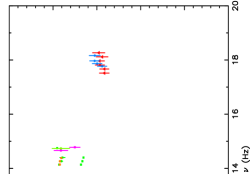
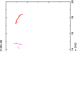
Fig. 2.: a- Spectral Energy Distribution of the BL Lacs 1ES 0033+595, PKS 0048$-$097, 1ES 0120+340 and RGB J0136+39

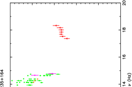
Fig. 2.: b- Spectral Energy Distribution of the BL Lacs 1ES 0145+138, MS 0158.5+0019, 3C 66A and AO 0235+164

Fig. 2.: c- Spectral Energy Distribution of the BL Lacs MS 0317.0+1834, 1H 0323+022, 1ES 0347$-$121 and 1H 0414+009

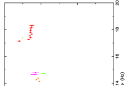
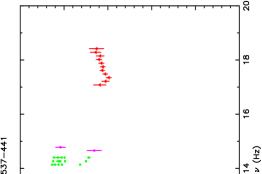
Fig. 2.: d- Spectral Energy Distribution of the BL Lacs 1ES 0502+675, 1H 0506$-$039, PKS 0521$-$365 and PKS 0537$-$441

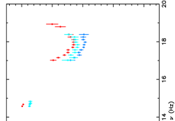
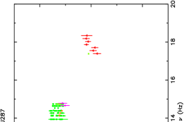
Fig. 2.: e- Spectral Energy Distribution of the BL Lacs PKS 0548$-$322, S5 0716+714, MS 0737.9+7441 and OJ 287

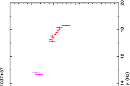
Fig. 2.: f- Spectral Energy Distribution of the BL Lacs B2 0912+29, 1ES 0927+500, 1ES 1028+511 and RGB J1037+57

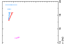
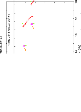
Fig. 2.: g- Spectral Energy Distribution of the BL Lacs RGB J1058+56, 1H 1100$-$230, Mkn 421 and 1RXS J111706.3+20141

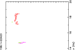
Fig. 2.: h- Spectral Energy Distribution of the BL Lacs EXO 1118.0+4228, Mkn 180, PKS 1144$-$379 and 1RXS J121158.1+22423

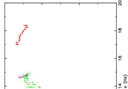
Fig. 2.: i- Spectral Energy Distribution of the BL Lacs EXO 1215.3+3022, 1H 1219+301, ON 231 and 1RXS J123511.1$-$14033

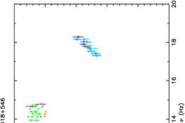
Fig. 2.: j- Spectral Energy Distribution of the BL Lacs 1ES 1255+244, MS 1312.1$-$4221, EXO 1415.6+2557 and PG 1418+546

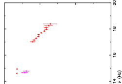
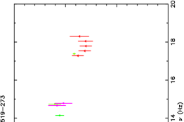
Fig. 2.: k- Spectral Energy Distribution of the BL Lacs 1H 1430+423, MS 1458.8+2249, 1H 1515+660 and PKS 1519$-$273

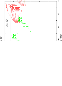
Fig. 2.: l- Spectral Energy Distribution of the BL Lacs 1ES 1533+535, 1ES 1544+820, 1ES 1553+113 and Mkn 501

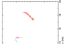
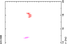
Fig. 2.: m- Spectral Energy Distribution of the BL Lacs 1ES 1741+196, S5 1803+784, 3C 371 and S4 1823+568

Fig. 2.: n- Spectral Energy Distribution of the BL Lacs 1ES 1959+650, PKS 2005$-$489, PKS 2155$-$304 and BL Lacertae

Fig. 2.: o- Spectral Energy Distribution of the BL Lacs 1ES 2344+514 and 1H 2354$-$315

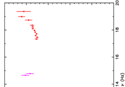
Fig. 3.: a- Spectral Energy Distribution of the FSRQs PKS 0208$-$512, NRAO 140, PKS 0523$-$33 and OG 147

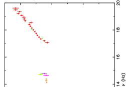
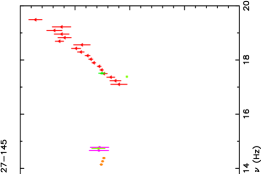
Fig. 3.: b- Spectral Energy Distribution of the FSRQs WGA J0546.6$-$6415, 1Jy 0836+710, RGB J0909+039 and 1Jy 1127$-$145

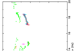
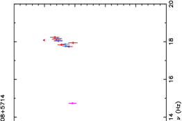
Fig. 3.: c- Spectral Energy Distribution of the FSRQs 3C 273, 3C 279, B3 1428+422 and GB 1508+5714

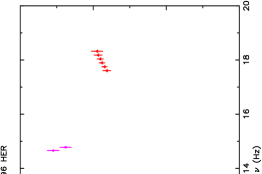
Fig. 3.: d- Spectral Energy Distribution of the FSRQs PKS 1510$-$08, 1ES 1627+402, 3C 345 and V 396 HER

Fig. 3.: e- Spectral Energy Distribution of the FSRQs 4C 62.29, S5 2116+81, PKS 2126$-$15 and OX 57

Fig. 3.: f- Spectral Energy Distribution of the FSRQs 1Jy 2149$-$306, PKS 2223+21, 3C 446 and CTA 102

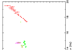
Fig. 3.: g- Spectral Energy Distribution of the FSRQs PKS 2243$-$123 and 3C 454.3

4 Summary and Conclusion

We have presented the X-ray spectrum and the Spectral Energy Distribution of a large sample of blazars observed by BeppoSAX with the aim of providing a single homogeneous reference for this type of BeppoSAX data. The collection of the results presented here together with all the data is also available as part of the BeppoSAX archive at the ASI Science Data Center (ASDC) at the following address

http://www.asdc.asi.it/blazars/

Given the heterogeneous nature of the sample we have not attempted to perform any deep statistical studies. In the following we summarize our work and give some remarks about possible interpretations. More detailed statistical studies or deeper interpretations are reported elsewhere or will be the subject of future publications.

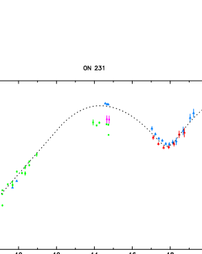
Fig. 4.: Spectral energy distributions of a typical LBL object (PG 1418+546, $\nu_{peak}$ $\approx 0.4~{}$eV$~{}\approx 8\times 10^{13}$Hz) for which the X-ray emission is dominated by the flat inverse Compton radiation and of an Intermediate BL Lac (ON 231, $\nu_{peak}$ $\approx 1~{}$eV$~{}\approx 2\times 10^{14}$Hz) where the simultaneous optical and BeppoSAX observations (Tagliaferri et al. 2000) clearly show that the transition between the synchrotron and inverse Compton emission occurs in the soft X-ray band.

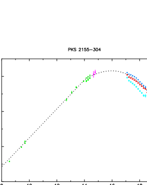
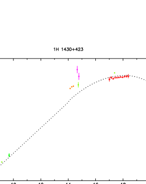
Fig. 5.: Spectral energy distributions of HBLs where the X-ray emission is completely dominated by synchrotron radiation. In the case of PKS 2155$-$304 $\nu_{peak}$ is at $\approx$ 50 eV $\approx\times 10^{16}$ Hz while for the extreme HBL 1H 1430+423 $\nu_{peak}$ is above 10 keV.

Fig. 6.: The distribution of the synchrotron peak frequencies in the FSRQ and in the BL Lac subsamples. While the $\nu_{peak}$ values for FSRQs strongly cluster around $10^{14}$ Hz, a much wider distribution is present in the BL Lacs subsample. In the latter case the distribution is strongly biased towards high $\nu_{peak}$ values by the BeppoSAX time allocation process which favoured X-ray bright (and therefore high $\nu_{peak}$ ) objects that could be detected by all NFI instruments.

The SED of the 84 blazars considered in this work confirms with large statistics the widely accepted scenario where blazar emission is smooth across several decades of energy and is characterized (in a $\nu f(\nu)~{}vs~{}\nu$ representation) by two broad peaks which are usually interpreted as being due to synchrotron emission followed by inverse Compton radiation.

A wide range of X-ray spectral indices has been observed, ranging from very flat values in Compton dominated sources like PG 1418+546 to very steep spectral slopes in objects where the tail of the synchrotron emission just reaches the X-ray band. A sharp transition from a very steep soft X-ray component to a much flatter hard X-ray spectrum, marking the transition between the synchrotron and Compton emission, has been clearly detected in a number of objects. Examples are given in Figures 4 and 5 where, for four representative objects, we plot the observed SED together with the expected distribution from a SSC model peaking at appropriate $\nu_{peak}$ values.

When viewed only from the narrow soft X-ray band, as was done in the past, these SEDs clearly show that the local X-ray spectral index must be correlated to the X-ray to radio flux ratio ($f_{x}/f_{r}$) as was first found by Padovani & Giommi (1996) and by Lamer, Brunner & Staubert (1996) in large samples of BL Lacs observed with ROSAT.

The position of the synchrotron peak, estimated comparing the SEDs to SSC models such as those shown in Figures 4 and 5, spans at least six orders of magnitudes ranging from $\approx 0.1~{}$eV in e.g. PKS 0048$-$097 or S5 2116+81 to 10–100 keV in some extreme HBL BL Lacs like Mkn 501 and 1H 1430+423.

Very strong intensity and spectral variability can occur near the synchrotron (and inverse Compton) peak. The position of this peak can move to higher energy by up to two orders of magnitude (or perhaps more) during flares.

It is not clear what is the maximum $\nu_{peak}$ that can be reached and whether Ultra High energy synchrotron peaked BL Lacs (UHBL) exist. A few potential UHBL sources may be present in the Sedentary survey (Giommi, Menna & Padovani 1999, Perri et al. 2002), which by definition only includes extreme HBL objects, especially those few that are located within the error circle of unidentified EGRET sources. If these candidates turn out to be the real counterpart of the EGRET gamma-ray sources their $\nu_{peak}$ would be so high that their synchrotron radiation would reach the gamma-ray band. One such object, 1RXS J123511.1$-$14033 (see Figure 2i), was observed by BeppoSAX on three occasions but always with short integration times giving inconclusive results (Giommi et al. 2002, in preparation).

The observed distributions of $\nu_{peak}$ values (rest frame), obtained by fitting SSC models to the multi-frequency data shown in Figure 2a-2o and 3a-3g, are plotted in Figure 6 for the FSRQ (top panel) and the BL Lac (bottom panel) subsamples. The two distributions are certainly affected by selection effects, including that induced by the BeppoSAX time allocation process which, by necessity, favoured high $\nu_{peak}$ /X-ray strong sources which could be detected by the high energy instruments. Although this bias is clearly present in the BL Lac subsample where a large fraction of the sources are X-ray bright HBL objects, in the case of FSRQs most of the objects have low $\nu_{peak}$ . This is because FSRQs are in general more luminous than BL Lacs and especially because FSRQs with $\nu_{peak}$ $>10^{16}$ Hz are very rare. To date the only FSRQ (RGB J1629+4008 = 1ES 1627+402, see Figure 3d) whose synchrotron emission reaches the X-ray band was found by Padovani et al. 2002b.

A logarithmic parabola model, which can describe the spectral curvature of blazars in a very wide energy band with only three parameters (see Landau et al. 1986), fits better than other models (e.g. broken power law) the spectrum of HBL objects whose X-ray emission is still due to synchrotron radiation. The average amount of spectral curvature, as measured by the $\beta$ parameter in the log parabola model of paragraph 3.1 is $-$0.38 +/$-$ 0.1, a value somewhat steeper (possibly because of the energy dependant synchrotron cooling), but not too different, than the amount of curvature found by Landau et al. 1986 ($-$0.22 to $-$0.09 ) in a sample of BL Lacs whose synchrotron power peaks at infra-red, optical frequencies. This similarity points to an intrinsically similar curvature in the spectrum of the emitting particles. The smoothly changing slope could be the spectral signature of a statistical acceleration mechanism where the acceleration process becomes less and less efficient as the particle’s energy increases (Massaro 2002). In this scenario the widely different synchrotron $\nu_{peak}$ energies in LBL and HBL objects would be the result of the inefficiency in the acceleration process that sets off at different energies.

References

- 1 Beckmann V., Wolter A. et al.: 2002, Astron. Astrophys. 383, 410
- 2 Ballo L., Maraschi L. et al.: 2002, Astrophys. J. 567, 50
- 3 Boella G. et al.: 1997a, Astron. Astrophys. Suppl. Ser. 122, 229
- 4 Boella G. et al.: 1997b, Astron. Astrophys. Suppl. Ser. 122, 327
- 5 Blandford R.D., Rees M.J.: 1978, in Pittsburgh Conf. on BL Lac objects, p. 328
- 6 Cardelli J.A., Clayton G.C., Mathis J.S.: 1989, Astrophys. J. 345, 245
- 7 Chiapetti L., Maraschi L. et al.: 1999, Astrophys. J. 521, 552
- 8 Costantini E., Comastri A. et al.: 1999, The Messenger 70, 265
- 9 Costamante L., Ghisellini G. et al.: 2001, Astron. Astrophys. 371, 512
- 10 Cusumano G., Mineo T. et al.: 2001, Astron. Astrophys. 375, 397
- 11 Dickey J.M., Lockman F.J.: 1990, Ann. Rew. Astron. Astrophys. 28, 215
- 12 Elvis M., Fiore F. et al.: 2000, Astrophys. J. 543, 545
- 13 Fabian A.C., Celotti A. et al.: 2001a, Mon. Not. R. Astr. Soc. 323, 373
- 14 Fabian A.C., Celotti A. et al.: 2001b, Mon. Not. R. Astr. Soc. 324, 628
- 15 Frontera F. et al.: 1997, Astron. Astrophys. Suppl. Ser. 122, 357
- 16 Fiore F., Guainazzi M., Grandi P.: 1999, Cookbook for NFI spectral analysis
- 17 Fossati G. et al.: 2000a, Astrophys. J. 541, 153
- 18 Fossati G. et al.: 2000b, Astrophys. J. 541, 166
- 19 Ghisellini G., Costamante L. et al.: 1999, Astron. Astrophys. 348, 63
- 20 Giommi P. et al.: 1990, Astrophys. J. 356, 432
- 21 Giommi P., Fiore F.: 1997, Data Analysis in Astronomy IV, p. 93
- 22 Giommi P., Fiore F. et al.: 1998, Astron. Astrophys. Lett. 333, L5
- 23 Giommi P., Massaro E. et al.: 1999, Astron. Astrophys. 351, 59
- 24 Giommi P., Menna M.T., Padovani P.: 1999, Mon. Not. R. Astr. Soc. 310, 465
- 25 Giommi P., Padovani P., Perlman E.: 2000 Mon. Not. R. Astr. Soc. 317, 743
- 26 Jager R. et al.: 1997, Astron. Astrophys. Suppl. Ser. 125, 557
- 27 Lamer G., Brunner H., Staubert R.: 1996, Astron. Astrophys. 311, 384
- 28 Landau R. et al.: 1986, Astrophys. J. 308, 78
- 29 Malizia A., Capalbi M. et al.: 2000, Mon. Not. R. Astr. Soc. 312, 123
- 30 Manzo G. et al.: 1997, Astron. Astrophys. Suppl. Ser. 122, 341
- 31 Massaro E., Cusumano G., Litterio M., Mineo, T.: 2000, Astron. Astrophys. 361, 695
- 32 Massaro E., Giommi P. et al.: 2002, Astron. Astrophys. submitted
- 33 Massaro E.: 2002, these proceedings
- 34 Morrison R., McCammon D.: 1983, Astrophys. J. 270, 119
- 35 Mineo T., Fiore F. et al.: 2000, Astron. Astrophys. 359, 471
- 36 Padovani P., Giommi P.: 1996, Mon. Not. R. Astr. Soc. 279, 526
- 37 Padovani P. et al.: 2001, Mon. Not. R. Astr. Soc. 328, 931
- 38 Padovani P. et al.: 2002a, Mon. Not. R. Astr. Soc. submitted
- 39 Padovani P. et al.: 2002b, Astrophys. J. submitted
- 40 Perri M., Giommi P., Piranomonte S., Padovani P.: 2002, these proceedings
- 41 Pian E. et al.: 1998, Astrophys. J. Lett. 492, L17
- 42 Pian E. et al.: 2002, Astron. Astrophys. 392, 407
- 43 Parmar A.N. et al.: 1997, Astron. Astrophys. Suppl. Ser. 122, 309
- 44 Ravasio M., Tagliaferri G. et al.: 2002, Astron. Astrophys. 383, 763
- 45 Siebert J., Brinkmann W. et al. : 1999, Astron. Nach. 320, 315
- 46 Tagliaferri G., Ghisellini G., Giommi P. et al.: 2000 Astron. Astrophys. 354, 431
- 47 Tavecchio F., Maraschi L., et al.: 2000, Astrophys. J. 543, 535
- 48 Tavecchio F. et al.: 2002, Astrophys. J. 575, 137
- 49 Tanihata C., et al.: 2001 Astrophys. J. 563, 569
- 50 Urry M.C., Padovani P.: 1995, Publ. Astr. Soc. Pacific 107, 803
- 51 Wolter A., Comastri A. et al.: 1998, Astron. Astrophys. 335, 899
- 52 Zhang Y.H., Celotti A. et al.: 1999, Astrophys. J. 527, 719
- 53