Stellar populations in local star-forming galaxies.
II.-Recent star formation properties and stellar masses.

Abstract

We present the integrated properties of the stellar populations in the Universidad Complutense de Madrid (UCM) Survey galaxies. Applying the techniques described in the first paper of this series, we derive ages, burst masses and metallicities of the newly-formed stars in our sample galaxies. The population of young stars is responsible for the $\rm H\alpha$ emission used to detect the objects in the UCM Survey. We also infer total stellar masses and star formation rates in a consistent way taking into account the evolutionary history of each galaxy. We find that an average UCM galaxy has a total stellar mass of $\sim 10^{10}\mathcal{M}_{\odot}$, of which about 5% has been formed in an instantaneous burst occurred about $5\,$Myr ago, and sub-solar metallicity. Less than 10% of the sample shows massive starbursts involving more than half of the total mass of the galaxy. Several correlations are found among the derived properties. The burst strength is correlated with the extinction and with the integrated optical colours for galaxies with low obscuration. The current star formation rate is correlated with the gas content. A stellar mass–metallicity relation is also found. Our analysis indicates that the UCM Survey galaxies span a broad range in properties between those of galaxies completely dominated by current/recent star formation and those of normal quiescent spirals. We also find evidence indicating that star-formation in the local universe is dominated by galaxies considerably less massive than $L^{*}$.

1 Introduction

The present paper is the second of a series which deals with the determination of the main properties of the stellar populations in the Universidad Complutense de Madrid (UCM) Survey galaxies (Zamorano et al., 1994, 1996; Alonso et al., 1999). We deal here with the integrated properties of the galaxies as a first step towards understanding their evolution. Future developments will address the properties of the spatially-resolved stellar populations and the improvement of the modelling procedures. This will be necessary to understand the details of the star formation history of each galaxy as well as their dust extinction properties, which turn out to be one of the key points (and probably the most important one) in this field.

One of the goals of this study is to determine the nature of the galaxies which were detected by the UCM Survey. There is an extensive dataset available for the sample, including spectroscopic and photometric information covering a broad wavelength range from the optical to the near infrared (nIR), together with some radio data. The analysis of the spectroscopic observations allow us to study the emission lines formed in the ionized gas clouds surrounding young hot stars. Among these lines, the Balmer $\rm H\alpha$ line is one of the best tracers of the most recent star formation (Kennicutt 1992, 1998a). It is easily observable in nearby galaxies and is less extinguished by dust than other optical emission lines ($\rm H\beta$, $\rm{[OII]}\lambda 3727$ Å) and the ultraviolet continuum. The $\rm H\alpha$ luminosity and equivalent width are directly linked to the youngest population of stars responsible for the heating and ionisation of the gas, and thus can be used in the determination of the mass in newly-formed stars, their age, etc. Spectroscopic data can also be used to evaluate the extinction (via the Balmer decrement), the metallicity, and the excitation.

Photometric data covering a wide wavelength range can be used to carry out a population synthesis analysis of composite stellar populations. Many examples of such studies, for low and high redshift galaxies, are found in the literature. See, e.g., Krüger et al. (1995); de Jong (1996); Abraham et al. (1999); Brinchmann & Ellis (2000); Gil de Paz et al. (2000a); Bell & de Jong (2000); Papovich et al. (2001). Some other authors have focused on the quantitative analysis of the optimal sets of observables and signal-to-noise ratios required to obtain robust results (see Bolzonella et al. 2000, and references therein; Gil de Paz & Madore 2002, and references therein).

In this respect, the combination of high-quality optical, ultraviolet and nIR data has been found provides some of the fundamental information needed to study local galaxies. To complement the broad-band photometry, emission-line fluxes can also be used in galaxies presenting star-formation activity. The ultraviolet part of the spectrum and the emission lines are dominated by young hot stars formed recently. The nIR is essential to characterise the more evolved population, since it is less sensitive to recent bursts and dust extinction.

One principal application of this line of research is the determination of the stellar masses of galaxies, another major goal of our project. It has been argued that nIR data, and more precisely, the K-band luminosity, can be used as a good tracer of the stellar mass (Rix & Rieke, 1993; Brinchmann & Ellis, 2000). Based on this assumption, several nIR-based surveys have been carried out in order to use the K-band luminosity function at several redshifts to directly obtain the distribution galaxy masses (e.g., Cowie et al. 1996; Cohen et al. 1999; Kochanek et al. 2001; Drory et al. 2001). However, it is very important to test the reliability of the stellar masses determined using $K$-band luminosities alone. Age differences from galaxy to galaxy, or the presence of massive recent star-formation (with a mass comparable to that of the evolved population) may have an effect on the mass-to-light ratio even in the nIR. Indeed, some authors have recently claimed that the K-band mass-to-light ratio depends on parameters such as the galaxy colours, clearly affecting the determination of total stellar masses (Moriondo et al., 1998; Brinchmann & Ellis, 2000; Bell & de Jong, 2001; Graham, 2002).

Pérez-González et al. (2002b, Paper I  hereafter) presented the dataset and the modelling and statistical techniques used in the current analysis. Paper I also discusses how well our techniques are able to reproduce the observations. Using a stellar population synthesis library, and taking into account the gas emission and dust attenuation, our method is able to model successfully the observational properties of star-forming galaxies. Several a priori parameters of the models were tested. These include (1) the evolutionary spectral synthesis library (we used Bruzual & Charlot –private communication– and Leitherer et al. 1999); (2) the recent star formation scenario (instantaneous and constant star formation rates -SFR- were tested); (3) the initial mass function (Salpeter 1955, Scalo 1986 and Miller & Scalo 1979); and (4) the extinction-correction recipe (Calzetti et al. 2000 and Charlot & Fall 2000). Among these, we found that the extinction plays a fundamental role.

We present now the results obtained from the application of our modelling procedure and statistical analysis to the UCM Survey data. Briefly, the global properties of the newly-formed stars and those of the underlying evolved population will be quantified. These properties are derived for each individual galaxy, ensuring that the stellar content and star formation history of each object are properly taken into account. The determination of these properties will lead to a better understanding of the observational biases of this kind of surveys.

A plan of the paper follows. First, the main properties of the UCM Survey sample will be briefly described in Section 2. The population synthesis method used in this will be reminded in Section 3 (see Paper I  for further details). Next, the results concerning the youngest population will be presented and discussed in Section 4. Following this, in Section 5 we will focus on the integrated stellar masses of the UCM galaxies. Finally, the conclusions will be presented. Throughout this paper we use a cosmology with $\mathrm{H}_{0}=70$ km s^-1 Mpc^-1, $\Omega_{\mathrm{M}}$=0.3 and $\Lambda$=0.7.

2 The sample

The present work has been carried out using the UCM Survey sample composed of 191 galaxies selected by their $\rm H\alpha$ emission at an average redshift of 0.026 (Zamorano et al., 1994, 1996; Gallego et al., 1996). Within this sample, 15 objects were classified as active galactic nuclei (AGN, including Sy1, Sy2 and LINER types) by Gallego et al. (1996), and have been excluded from this study. Another 11 galaxies were observed in only two bands and the comparison with the models was not attempted. The final sample is consequently formed by 163 galaxies (cf. Paper I).

The extensive dataset used in this work includes optical and nIR imaging, and optical spectroscopy. For more details on the observations and the main spectroscopic and photometric properties of the galaxies, see Paper I  and references therein.

Although not presented in Paper I, in this paper we will also make use of the available HI 21 cm data for the UCM Survey galaxies. These data were obtained from the NASA/IPAC Extragalactic Database (NED). Most of the 21 cm fluxes come from Huchtmeier & Richter (1989). We also used the data for 11 galaxies from Pisano et al. (2001). HI masses (in solar units) were calculated with the expression

$$\mathcal{M}_{HI}=2.356\cdot 10^{5}\cdot D^{2}$$\int Sd\nu,$$ (1)

where $D$ is the distance in Mpc and $\int Sd\nu$ is the integrated line-flux in Jy km s^-1 (Roberts, 1975).

3 Basic assumptions and methodology

Paper I  described the method to derive the properties of the most recent star-formation in star-forming galaxies using broad-band photometry and spectroscopy. Although the basic assumptions and methodology were extensively described in that paper, we summarise them here to make this paper as self-contained as possible. The technique is based on the assumption that these galaxies have a composite stellar population. The detection of nebular emission lines is undoubtedly a hint for the presence of a very young stellar population, which will be referred as a recent burst of star formation, the newly-formed stars or the recent starburst. This population is also responsible for the bluer colours observed in the UCM galaxies in comparison with ‘normal quiescent’ (relaxed) spirals (see Alonso-Herrero et al., 1996; Pérez-González et al., 2000).

This recent starburst is occurring in a spiral/lenticular galaxy. Morphological studies were carried out by Vitores et al. (1996) in the Gunn $r$ band and Pérez-González et al. (2001) in the Johnson $B$ band. A typical spiral intrinsically shows HII regions ionized by a population of recently-formed stars. Kennicutt (1983) and Davidge (1992) estimated the importance of this population (in comparison with the entire stellar content) measuring the $\mathrm{H}\alpha$ equivalent width for a sample of normal spirals. On average, a typical relaxed Sb galaxy presents a value of 8 Å. However, the detection limit of the UCM Survey is $EW(\rm H\alpha)\sim 20$ Å  (Gallego, 1995). Consequently, the UCM objects must be experiencing a stronger burst of star formation in comparison with a normal galaxy.

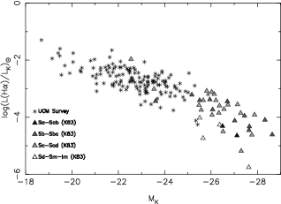
Figure 1 shows the distinct nature of the UCM galaxies and normal spirals (Kennicutt, 1998b). This plot depicts the stellar mass (as traced by the $K$-band luminosity) versus the luminosity from young stars (as traced by the $\mathrm{H}\alpha$ luminosity). The latter has been normalized with the $K$-band luminosity in order to be able to compare between objects with different luminosities/stellar masses. The nIR data for the comparison sample have been extracted from the Two Micron All Sky Survey (2MASS, Jarrett et al., 2000), NED and de Jong & van der Kruit (1994). UCM galaxies appear as fainter objects than normal spirals but presenting larger normalized $\mathrm{H}\alpha$ luminosities. This means that the present star formation is more important in comparison with the older population in the UCM objects than in normal spirals.

Figure 1: Comparison of the UCM objects (asterisks) with normal relaxed (quiescent) spiral/irregular galaxies (triangles; Kennicutt, 1998b). Vertical axis is plotted in solar units.

Our modelling refers to the properties of a recent star formation event which takes place in excess of what is typical in a normal spiral or lenticular galaxy. We have assumed that a recent burst of star formation (described by its age, metallicity and mass) is occurring in a galaxy whose colours and $EW(\rm H\alpha)$ are those of a typical galaxy of the same morphological type. The assumed colours of the underlying evolved (older) population, which have been taken from the literature, are the result of the past star formation history of these typical galaxies. The details of this past history are beyond the scope of this paper. Here we are not concerned with the detailed histories of individual galaxies, but with the statistical properties of our sample. The validity of this approach, at least in the statistical sense, is supported by the correlation between averaged colours and Hubble type for large samples of galaxies (see, e.g, Fukugita et al., 1995; Fioc & Rocca-Volmerange, 1999; Strateva et al., 2001). In addition, these underlying population colours are quite similar to our measurements in the outer parts of some randomly selected test galaxies (Pérez-González et al., 2002a).

The recent burst must be younger than $\sim 10$ Myr, since the $EW(\rm H\alpha)$ drops considerably for ages older than this value. Given this short period of time, the star formation may be approximated by an instantaneous or constant SFR burst. A possible scenario with multiple bursts occurring all through the galaxy would be mimicked by a constant SFR model.

This work also deals with the estimation of the total stellar mass of each galaxy. Mass-to-light ratios in the nIR (and in particular the $K$-band) have been claimed to be roughly independent of the galaxies’ stellar populations and star-formation histories (Rix & Rieke, 1993; Brinchmann & Ellis, 2000). This statement will be discussed in Section 5.

The modelling technique described in Paper I  yields three parameters describing the population of newly-formed stars in the UCM galaxies. The three parameters are the age $t$, metallicity $Z$ and burst strength $b$ (ratio between the mass of the starburst and the total stellar mass of the galaxy, i.e., the importance of the recent star formation event). Both the observed colours and equivalent width that are fitted by our modelling and the output parameters have been considered as statistical distributions. The method also includes a Principal Component Analysis on the space of solutions which takes account of the degeneracies in this kind of studies (cf. Paper I). The next sections will deal with the results obtained for these three properties.

Paper I  introduced and tested some input parameters that should be selected a priori. All of them refer to the stellar and nebular emission arising from the recent starburst. As a reminder, we list here these parameters and the acronyms used hereafter:

• The evolutionary synthesis model: Bruzual & Charlot (1999, private communication; BC99 hereafter) or Leitherer et al. (1999, SB99  from now on).

• The star-forming mode of the young stellar population: instantaneous or continuous star formation rate. These modes will be referred to as INST and CONS.

• The IMF: Salpeter (1955, SALP), Scalo (1986, SCA), or Miller & Scalo (1979, MSCA). In all cases, we use $\mathcal{M}_{\mathrm{low}}=0.1\,\mathcal{M}_{\odot}$ and $\mathcal{M}_{\mathrm{up}}=100\,\mathcal{M}_{\odot}$ for the lower and upper mass limits of the IMF.

• The extinction recipe: Calzetti et al. (2000, CALZ00) or Charlot & Fall (2000, CF00).

4 Properties of the young stellar population

4.1 Burst strength

Figure 2: Distribution of the burst strengths derived for the UCM Survey galaxies. BC99 instantaneous SFR models for the three initial mass functions and the CF00  extinction recipe are plotted on the left and constant SFR models on the right. Each row corresponds to each one of the three IMFs considered: Salpeter (SALP), Scalo (SCA) and Miller-Scalo (MSCA).

Fig. 2 shows the histograms of the burst strength (in a logarithmic scale) for the 3 IMFs considered and the CF00  extinction recipe. Left panels show results for the INST star formation and right panels for the CONS case. On the top of each diagram, the median value and quartiles are drawn. These quantities are also given in Table 1, together with the relevant values for the rest of the derived quantities. The median values of the burst strengths are 2–12%, depending on the input parameters of the models. The individual values of $b$ cover the whole range considered, from a pure young bursts ($b\simeq 1$) to masses of new stars that are less than 1% of the total mass of the galaxy. These results are similar to what was found for a smaller subsample in Gil de Paz et al. (2000a, hereafter GdP00), albeit with some of the galaxies studied now showing burst strengths close to 100%. These high-$b$ objects were not present in the subsample studied by GdP00.

The models with SCA and MSCA IMFs present higher values of the burst strength than those using SALP by up to a factor of 3–5. For the same age, the SCA models are redder than the MSCA ones, and these in turn are redder than the SALP ones. More young stars need to be added to the redder models in order to account for the observed colours, and the derived burst strength rises.

The burst strengths derived using a constant SFR and an instantaneous burst are compared in Fig. 3. The points scatter around the 1–to–1 line for all the IMFs. This indicates that, after a few million years, the observed properties of a galaxy that experienced a massive instantaneous burst will resemble those of one experiencing a less efficient but longer star formation event in which the mass of newly-formed stars is similar. We will come to this fact later. Galaxies show a small tendency to to have lower values of $b$ for the CONS case than for the INST one. Indeed, for a given age, one can reproduce a certain $EW(\rm H\alpha)$ with a continuous burst less massive than an instantaneous one. The good agreement between the $b$ values derived with the INST and CONS models for the galaxies with the lowest burst strengths is remarkable. These objects also show similarly young burst ages for both star-formation scenarios (see Section 4.2).

Figure 3: Comparison of burst strengths for instantaneous and constant rates of star-formation. The points refer to the BC99 code, CF00  extinction recipe and the 3 IMFs described in the text.

A comparison of the CONST and INST burst strengths derived for the SB99  models with the CF00  extinction law is presented in Fig. 6, with very similar conclusions. On average, SB99  models show higher burst strengths than BC99 ones by a factor of 0.1-0.2dex for case of CF00  extinction and lower for the CALZ00  prescription.

In Paper I  we concluded that the vast majority of the UCM galaxies are better fitted with the INST models than with the CONS ones. Thus, the $b$ values derived from the best-fitting models will refer, in most cases, to the instantaneous burst scenario.

Only 5 objects have burst strengths higher than 50% as derved from more than one model, including the model that best reproduces the observations. Four more join this group if we only consider the best-fitting model. Out of these 9 objects, 4 are classified as SBN (Gallego et al., 1996, see Paper I  for a short description), two as DANS and three as HIIH objects. Most of them are compact objects (e.g., UCM1256$+$2910, UCM2315$+$1923 and UCM2319$+$2234), some have extended star-formation located throughout the object (as seen in $\rm H\alpha$ imaging presented in Pérez-González et al., 2002c, e.g., UCM0022+2049 and UCM1306$+$3111). There are also two face-on galaxies with clear spiral arms and a massive nuclear burst (UCM2256$+$2001 and UCM2317$+$2356). All 9 galaxies having stellar populations dominated by the young stars have relatively high extinctions, i.e., $E(B-V)=0.6-1.5$.

4.2 Age

Figure 4: Distribution of the ages derived for the UCM Survey galaxies. BC99 instantaneous SFR models for the three initial mass functions and CF00  extinction are plotted on the left and constant star formation rate models on the right.

The derived burst ages for the UCM galaxies show a relatively narrow peak at 5–6 Myr for INST models (Fig. 4, left). The median age and age distribution for the entire sample is almost independent of the IMF considered. The difference in mean age is only 0.01dex for the three IMFs. The independence of the derived burst ages on the IMF can be easily explained. The most important observable when determining the age of a young stellar population is $EW(\rm H\alpha)$ (cf. Alonso-Herrero et al. 1996, GdP00). The $EW(\rm H\alpha)$ for young stellar populations is dominated by the most massive stars present, and thus the $EW(\rm H\alpha)$ ‘clock’ only depends on the evolutionary clock of these massive stars, which doesn’t depend on the IMF.

The reason for the narrow burst age distributions derived for the UCM galaxies can be explained from the way UCM galaxies were selected (see also discussion on Section 4.4). Only objects with relatively high $\rm H\alpha$ equivalent widths ($>20\,$Å) are present in the sample (Gallego, 1995). Since $EW(\rm H\alpha)$ drops sharply below that value after $\sim 10$ Myr (Fig. 8), a sharp cutoff in the age distribution is expected at that age. The logarithmic nature of the $x$ axis in Fig. 4 partially explains the drop in galaxy numbers for ages below $3\,$Myr, since the time intervals encompassed by the low age bins is smaller. Moreover, for these very young ages the burst of star-formation is probably still hidden in very-high extinction regions (Gordon et al., 1997), and therefore galaxies with very young bursts will be hard to detect.

The ages of the young stellar populations derived for the constant SFR models are not well constrained since $EW(\rm H\alpha)$ changes very slowly with age (Alonso-Herrero et al., 1996). The derived age distribution appears to be rather flat for these models (Fig. 4, right). The apparent excess of galaxies with older ages ($\log(t)\sim 8$) is mainly due to the large time interval encompassed by the last bin. In any case, since the UCM galaxies clearly favour the INST models, the ages derived from the CONS models are largely irrelevant.

When comparing BC99 and SB99  models (see Fig. 6, middle-left panel), marginally younger burst ages (by 0.1dex) are found for the former, but the age distributions are similar. This behaviour derives directly from the fact that the predicted $EW(\rm H\alpha)$ at any given age is higher in the SB99  case. This is due to the different evolutionary tracks and stellar libraries used in both sets of population synthesis models.

Table 1: Median values and quartiles of the derived burst strengths, ages and metallicities.

$\log(t)$

$\log(b)$

$\log(Z)$

Bruzual & Charlot 1999

INST

CONS

INST

CONS

INST

CONS

SALP

CF00

6.71

${}^{+0.13}_{-0.11}$

7.45

${}^{+0.50}_{-0.59}$

$-$1.53

${}^{+0.33}_{-0.39}$

$-$1.80

${}^{+0.60}_{-0.53}$

$-$0.16

${}^{+0.33}_{-0.27}$

$-$0.04

${}^{+0.32}_{-0.36}$

CALZ00

6.75

${}^{+0.08}_{-0.13}$

7.60

${}^{+0.34}_{-0.56}$

$-$1.83

${}^{+0.42}_{-0.37}$

$-$1.77

${}^{+0.27}_{-0.67}$

$-$0.18

${}^{+0.21}_{-0.20}$

$-$0.20

${}^{+0.31}_{-0.24}$

SCA

CF00

6.70

${}^{+0.14}_{-0.10}$

7.67

${}^{+0.28}_{-0.67}$

$-$0.92

${}^{+0.29}_{-0.35}$

$-$0.98

${}^{+0.40}_{-0.51}$

$-$0.16

${}^{+0.33}_{-0.26}$

$-$0.18

${}^{+0.33}_{-0.25}$

CALZ00

6.74

${}^{+0.08}_{-0.14}$

7.46

${}^{+0.36}_{-0.46}$

$-$1.24

${}^{+0.31}_{-0.30}$

$-$1.21

${}^{+0.32}_{-0.54}$

$-$0.16

${}^{+0.19}_{-0.20}$

$-$0.24

${}^{+0.23}_{-0.22}$

MSCA

CF00

6.70

${}^{+0.14}_{-0.09}$

7.49

${}^{+0.42}_{-0.55}$

$-$1.12

${}^{+0.26}_{-0.40}$

$-$1.17

${}^{+0.49}_{-0.43}$

$-$0.16

${}^{+0.30}_{-0.24}$

$-$0.26

${}^{+0.31}_{-0.17}$

CALZ00

6.75

${}^{+0.08}_{-0.13}$

7.22

${}^{+0.44}_{-0.32}$

$-$1.54

${}^{+0.34}_{-0.31}$

$-$1.51

${}^{+0.41}_{-0.54}$

$-$0.17

${}^{+0.16}_{-0.21}$

$-$0.20

${}^{+0.23}_{-0.23}$

Leitherer et al. 1999

INST

CONS

INST

CONS

INST

CONS

SALP

CF00

6.79

${}^{+0.11}_{-0.11}$

7.92

${}^{+0.07}_{-0.45}$

$-$1.36

${}^{+0.41}_{-0.42}$

$-$1.60

${}^{+0.45}_{-0.33}$

$-$0.54

${}^{+0.44}_{-0.44}$

$-$0.55

${}^{+0.38}_{-0.53}$

CALZ00

6.71

${}^{+0.07}_{-0.15}$

7.76

${}^{+0.21}_{-0.43}$

$-$1.95

${}^{+0.43}_{-0.33}$

$-$1.66

${}^{+0.35}_{-0.64}$

$-$0.35

${}^{+0.30}_{-0.34}$

$-$0.44

${}^{+0.50}_{-0.23}$

Best Fit

$\log(t)$

$\log(b)$

$\log(Z)$

6.79

${}^{+0.08}_{-0.07,}$

$-$1.31

${}^{+0.44}_{-0.37}$

$-$0.04

${}^{+0.13}_{-0.23}$

Table 1: Median values and quartiles are shown for the three parameters fitted by our models. All the possible input choices are shown. The last 2 rows give the median values and quartiles of the best fits for each galaxy.

4.3 Metallicity

As discussed in GdP00  and Paper I, the metallicity has a smaller effect on the colours and $EW(\rm H\alpha)$’s predicted by the models than the burst strength and the age. Thus, the model-derived metallicities are much more uncertain. Moreover, the population synthesis models used have metallicities with a small number of discrete values, which has a very strong effect in the clustering of solutions in the parameter space (GdP00, Paper I). Although for the sake of completeness we will present in this section the metallicities derived by the models, extreme caution is needed when interpreting the results.

Fig. 5 shows the distribution of model-derived metallicities for the young populations in the UCM sample galaxies. There is a large spread in the metallicities fitted by our models, with more galaxies with metallicities below solar than above. The mean metallicity derived with the different models is $\langle\log(Z/Z_{\odot})\rangle\simeq-0.2$. The derived metallicities are almost independent of the IMF considered.

Figure 5: Distribution of the model-derived metallicity for the UCM Survey galaxies. BC99 instantaneous SFR models for the three initial mass functions and CF00  extinction prescription are plotted on the left and constant SFR models on the right.

Figure 6: Distribution of young population parameters for the UCM Survey galaxies. SB99  instantaneous SFR models and CF00  extinction are plotted on the left and constant SFR models on the right.

Finally, SB99  models (Fig. 6, lower panels) give lower metallicity values by 0.3–0.5dex, leaving less than 10% of the objects with metallicities above solar.

In section 5 we will discuss the spectroscopically-derived chemical abundance of the gas and its correlation with the galaxies’ stellar masses.

4.4 Correlations

For the sake of simplicity, in this section and the reminder of this paper, all the plots will refer to the results obtained with the CF00  extinction recipe, SB99  models with instantaneous SFR and a Salpeter IMF. As discussed in Paper I, this choice yields the best results when modelling the data, although the CALZ00  extinction recipe seems to work marginally better for high extinction objects. In the plots, only galaxies with acceptable fits (as defined in Paper I) will be shown. When relevant, results obtained with different model parameter choices will also be mentioned in the discussion, including the set of results corresponding to the best-fitting model for each galaxy.

Fig. 7 shows the distribution of burst strengths according to the morphological type of each galaxy. Median values are indicated. The results for the SB99  models suggest a relative modest increase in burst strength from Sa to Sc$+$. The number of galaxies classified as irregulars is too small to infer firm results. Although this behaviour agrees with the idea that star formation is relatively more important in late spirals than in earlier ones, we remind the reader that our models assume an underlying stellar population in each galaxy similar to that of a ‘normal’ galaxy with the same morphological type. Thus, $b$ refers to new stars formed in excess of what an average galaxy with the same morphological type would have (cf. Paper I). Another important point to remember when considering morphological trends is that the UCM sample is biased against low surface brightness objects, since the galaxies were selected from objective-prism photographic plates. Moreover, for an S0 galaxy to be detected in $\rm H\alpha$, its star formation must be significantly enhanced with respect to a ‘normal’ S0. It is also worth pointing that the relatively low burst strengths derived for Blue Compact Dwarf galaxies ($\langle b\rangle\simeq 5$%) reveals the presence of an important underlying stellar population (Krüger et al., 1995; Gil de Paz et al., 2000b, c; Kunth & Östlin, 2000).

Figure 7: Histograms of the burst strength for the UCM galaxies divided according to Hubble type (Pérez-González et al., 2001). INT denotes interacting galaxies, and BCD Blue Compact Dwarf galaxies. Instantaneous SFR for SB99  models, Salpeter IMF and CF00  extinction is plotted on the left and the distribution of best-fittings on the right.

Fig. 8 shows the relationship between model-derived age and $EW(\rm H\alpha)$ for the UCM galaxies. We use different symbols for objects with different $\log(b)$ values. Models for solar metallicity and several burst strengths (with an underlying population of a Sb galaxy, the most common morphology of the sample) have also been plotted. Both the models and the data show that for ages above $\sim 2\,$Myr, the $EW(\rm H\alpha)$ decreases with age. This is hardly surprising, since, as discussed above, $EW(\rm H\alpha)$ provides the strongest constraint when determining the ages. Given that at $\sim 10\,$ Myr the EW of the young stars equals the EW of the underlying stellar population, the model predictions cross at that age. For older ages, the $EW(\rm H\alpha)$ for the composite stellar population becomes constant with time. For very low burst strengths ($\log(b)\simeq-3$), $EW(\rm H\alpha)\simeq 8\,$Å, i.e., the value corresponding to the underlying stellar population. For higher $b$ values, $EW(\rm H\alpha)$ is dominated by the newly-formed stars, which have lower $EW$s.

Figure 8: Time evolution of the $\rm H\alpha$ equivalent width for solar metallicity models and different burst strengths. Derived values for the UCM sample are also shown. Different symbols are used for galaxies with different $\log(b)$. Note that some of the points have $\log(b)$ values outside the range span by the models, but his is due to the fact that only solar metallicity models with a fixed underlying population are shown. If we had plotted the full range of models used, the models would encompass the full range of derived $\log(b)$ values (by construction).

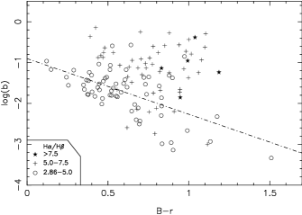
In Fig. 9 we draw the $\rm H\alpha/\rm H\beta$ ratio (a measure of extinction) versus the burst strength as derived with our method. Although a large scatter is present, the galaxies with the largest values of $b$ seem to have typically larger extinctions, with $\rm H\alpha/\rm H\beta$ ratios above 5.0, i.e., $E(B-V)>0.5$. Galaxies with smaller bursts, on the other hand, seem to inhabit objects with lower extinction.

Figure 9: Burst strength as a function of the extinction (represented by the $\rm H\alpha/\rm H\beta$ ratio, Gallego et al. 1996). The histograms show the distribution of the burst strengths for disk-like and HII-like galaxies.

In Fig. 9 we have inlaid histograms showing the distribution of burst strengths according to the galaxies’ spectroscopic type (see Gallego et al., 1996, and Section 2.3 of Paper I). The distributions are quite similar.

Figure 10: Burst strength vs. $B-r$ colour for the UCM Survey galaxies. Information about extinction ($\rm H\alpha/\rm H\beta$ ratio) is indicated with different symbols. A fit to the low-extinction points ($\rm H\alpha/\rm H\beta<5$) is shown by the dashed line. The equation of this fit is $\log(b)=(-0.90\pm 0.16)+(-1.36\pm 0.24)\cdot(B-r)$, with a scatter $\sigma=0.47$. If we use the CALZ00  extinction recipe, the fit would have a lower zero-point, but very similar slope, i.e., $\log(b)=(-1.30\pm 0.13)+(-1.37\pm 0.21)\cdot(B-r)$, with a scatter $\sigma=0.42$.

Finally, Fig. 10 presents $\log(b)$ against the $B-r$ integrated colour of the galaxies corrected for Galactic extinction. There is a clearly-defined lower envelope in the distribution of points, indicating that there are no blue objects with low burst strengths. Indeed, for galaxies with low extinction ($\rm H\alpha/\rm H\beta<5$), there is a clear anti-correlation between burst strength and colour. As expected, bluer objects have larger $b$ values. Note that most of these objects have $b<10$%, even though they can be very blue, almost reaching $B-r\sim 0.0$. Objects with higher extinction ($\rm H\alpha/\rm H\beta>5$) have, typically, larger values of $b$ than the less extincted ones for a given colour. No trend can be seen for these objects. Although for them one would expect that large $b$ values would imply bluer colours, different extinctions would make the colours redder by different amounts, adding scatter and thus hiding any possible trend. It is thus clear that with optical colours alone, only lower limits in $b$ can be derived.

Table 2: Stellar population synthesis results for the UCM Survey galaxies.

UCM name	$\log(t)$	$\log(b)$	$\log(Z)$	$\mathcal{M}/L_{K}$	$\log(\mathcal{M}_{*}/\mathcal{M}_{\odot})$	$\log(SFR/\mathcal{M}_{*})$	PCA	Var
(1)	(2)	(3)	(4)	(5)	(6)	(7)	(8)	(9)	(10)
0000$+$2140	6.59$\pm$0.08	$-$0.97$\pm$0.23	$-$0.07$\pm$0.63	0.31$\pm$0.07	10.90$\pm$0.10	$-$	($+$0.404,$+$0.634,$+$0.660)	60.7
	7.10$\pm$0.35	$-$1.11$\pm$0.22	$+$0.10$\pm$0.41	0.29$\pm$0.02	10.87$\pm$0.03	$-$	($+$0.573,$+$0.574,$-$0.585)	94.1	7
0003$+$2200	6.79$\pm$0.08	$-$1.04$\pm$0.77	$-$0.11$\pm$0.23	0.18$\pm$0.21	9.28$\pm$0.49	2.65$\pm$0.49	($+$0.610,$+$0.571,$-$0.549)	87.1
0006$+$2332	6.81$\pm$0.09	$-$0.94$\pm$0.29	$-$0.20$\pm$0.48	0.28$\pm$0.16	9.82$\pm$0.25	$-$	($+$0.684,$+$0.298,$-$0.666)	69.0
	6.75$\pm$0.03	$-$1.28$\pm$0.32	$-$0.03$\pm$0.23	0.30$\pm$0.14	9.84$\pm$0.20	$-$	($+$0.695,$+$0.718,$+$0.027)	47.5	29
0013$+$1942	6.75$\pm$0.13	$-$1.88$\pm$0.23	$-$0.79$\pm$0.69	0.61$\pm$0.02	9.70$\pm$0.03	2.73$\pm$0.03	($+$0.605,$+$0.560,$-$0.566)	89.0
	6.71$\pm$0.22	$-$1.83$\pm$0.80	$-$0.18$\pm$0.41	0.34$\pm$0.38	9.43$\pm$0.48	3.00$\pm$0.48	($+$0.712,$+$0.701,$-$0.040)	59.7	17
0014$+$1829	6.11$\pm$0.14	$-$1.93$\pm$0.13	$-$1.30$\pm$0.00	0.86$\pm$0.02	10.11$\pm$0.07	2.13$\pm$0.07	($-$0.707,$+$0.707,$+$0.001)	37.7	$\chi^{2}>4$
	6.41$\pm$0.08	$-$0.71$\pm$0.28	$+$0.37$\pm$0.16	0.27$\pm$0.13	9.61$\pm$0.23	2.63$\pm$0.23	($+$0.616,$+$0.489,$-$0.618)	65.7	17
0014$+$1748	6.36$\pm$0.22	$-$2.21$\pm$0.52	$-$0.41$\pm$0.69	0.62$\pm$0.22	10.74$\pm$0.17	2.22$\pm$0.17	($+$0.620,$+$0.639,$+$0.455)	68.5
	6.71$\pm$0.39	$-$1.26$\pm$1.09	$-$0.09$\pm$0.29	0.13$\pm$0.19	10.07$\pm$0.62	2.89$\pm$0.62	($+$0.605,$+$0.603,$+$0.520)	79.7	17
0015$+$2212	6.66$\pm$0.13	$-$2.43$\pm$0.27	$-$0.79$\pm$0.66	0.89$\pm$0.04	9.93$\pm$0.03	2.56$\pm$0.03	($+$0.684,$+$0.595,$-$0.421)	69.9
	6.76$\pm$0.24	$-$2.03$\pm$0.59	$-$0.03$\pm$0.34	0.55$\pm$0.31	9.72$\pm$0.24	2.76$\pm$0.24	($+$0.713,$+$0.676,$-$0.188)	63.1	1
0017$+$1942	6.87$\pm$0.11	$-$1.04$\pm$0.19	$-$0.93$\pm$0.53	0.49$\pm$0.13	10.02$\pm$0.12	2.69$\pm$0.12	($+$0.653,$+$0.463,$-$0.599)	75.8
	6.67$\pm$0.08	$-$1.64$\pm$0.26	$-$0.07$\pm$0.55	0.48$\pm$0.13	10.01$\pm$0.12	2.70$\pm$0.12	($+$0.758,$+$0.401,$-$0.515)	54.9	29
0017$+$2148	6.82$\pm$0.11	$-$1.24$\pm$0.58	$-$0.69$\pm$0.65	0.41$\pm$0.47	9.60$\pm$0.50	$-$	($-$0.627,$+$0.337,$+$0.702)	65.6
	6.81$\pm$0.19	$-$1.62$\pm$0.62	$+$0.12$\pm$0.29	0.31$\pm$0.31	9.48$\pm$0.44	$-$	($+$0.751,$+$0.640,$-$0.163)	49.8	17
0018$+$2216	6.80$\pm$0.02	$-$2.11$\pm$0.14	$+$0.21$\pm$0.20	0.54$\pm$0.05	9.49$\pm$0.05	1.95$\pm$0.05	($-$0.708,$-$0.008,$+$0.707)	62.2
	6.85$\pm$0.02	$-$1.71$\pm$0.44	$+$0.19$\pm$0.20	0.29$\pm$0.21	9.22$\pm$0.32	2.22$\pm$0.32	($-$0.480,$+$0.490,$+$0.727)	58.4	29
0018$+$2218	7.01$\pm$0.15	$-$0.34$\pm$0.42	$-$0.89$\pm$0.61	0.37$\pm$0.10	10.66$\pm$0.14	$-$	($+$0.589,$+$0.561,$-$0.582)	94.1
0019$+$2201	6.82$\pm$0.03	$-$1.31$\pm$0.68	$+$0.00$\pm$0.02	0.18$\pm$0.22	9.30$\pm$0.54	2.70$\pm$0.54	($+$0.706,$+$0.706,$-$0.061)	59.4
0022$+$2049	6.69$\pm$0.15	$-$1.25$\pm$0.40	$-$0.09$\pm$0.31	0.32$\pm$0.15	10.35$\pm$0.21	2.41$\pm$0.21	($+$0.620,$+$0.550,$+$0.560)	83.9
	7.79$\pm$0.15	$-$0.29$\pm$0.21	$-$0.63$\pm$0.16	0.09$\pm$0.02	9.81$\pm$0.11	2.95$\pm$0.11	($+$0.608,$+$0.585,$-$0.537)	68.7	11
0023$+$1908	6.79$\pm$0.12	$-$1.01$\pm$0.54	$-$0.53$\pm$0.66	0.25$\pm$0.27	9.35$\pm$0.46	$-$	($-$0.655,$+$0.240,$+$0.716)	61.6
0037$+$2226	6.90$\pm$0.12	$-$1.07$\pm$0.58	$-$0.67$\pm$0.64	0.28$\pm$0.35	10.14$\pm$0.55	$-$	($-$0.643,$+$0.369,$+$0.671)	70.9
	6.84$\pm$0.12	$-$1.77$\pm$0.32	$-$0.59$\pm$0.62	0.53$\pm$0.24	10.42$\pm$0.20	$-$	($+$0.681,$+$0.379,$-$0.627)	69.6	29
0038$+$2259	6.80$\pm$0.11	$-$1.13$\pm$0.45	$+$0.12$\pm$0.46	0.30$\pm$0.24	10.33$\pm$0.35	2.18$\pm$0.35	($+$0.689,$+$0.268,$-$0.674)	68.4
	6.80$\pm$0.03	$-$1.51$\pm$0.46	$+$0.00$\pm$0.14	0.31$\pm$0.23	10.35$\pm$0.32	2.17$\pm$0.32	($+$0.722,$+$0.366,$-$0.588)	55.6	29
0040$+$0257	7.00$\pm$0.02	$-$0.87$\pm$0.06	$-$1.30$\pm$0.00	0.62$\pm$0.01	9.84$\pm$0.03	2.69$\pm$0.03	($+$0.707,$+$0.707,$-$0.001)	46.3	$\chi^{2}>4$
	6.65$\pm$0.06	$-$0.98$\pm$0.64	$+$0.40$\pm$0.04	0.12$\pm$0.16	9.12$\pm$0.58	3.41$\pm$0.58	($+$0.710,$+$0.696,$-$0.106)	54.5	17
0040$+$2312	6.92$\pm$0.12	$-$0.38$\pm$0.37	$-$0.68$\pm$0.50	0.27$\pm$0.09	10.65$\pm$0.14	$-$	($+$0.586,$+$0.561,$-$0.584)	93.5
0040$+$0220	6.82$\pm$0.13	$-$1.42$\pm$0.25	$-$0.55$\pm$0.73	0.52$\pm$0.15	9.19$\pm$0.13	2.69$\pm$0.13	($+$0.621,$+$0.526,$-$0.581)	84.5
0043$-$0159	6.15$\pm$0.15	$-$2.26$\pm$0.19	$-$1.30$\pm$0.00	0.64$\pm$0.01	11.14$\pm$0.03	$-$	($-$0.707,$+$0.707,$+$0.001)	37.6	$\chi^{2}>4$
	6.59$\pm$0.12	$-$0.47$\pm$0.43	$+$0.39$\pm$0.06	0.14$\pm$0.10	10.48$\pm$0.32	$-$	($+$0.708,$+$0.706,$-$0.022)	61.4	19
0044$+$2246	6.79$\pm$0.09	$-$0.63$\pm$0.50	$+$0.00$\pm$0.44	0.19$\pm$0.12	10.29$\pm$0.28	2.23$\pm$0.28	($+$0.710,$+$0.128,$-$0.692)	65.2
0045$+$2206	6.74$\pm$0.12	$-$1.59$\pm$0.49	$-$0.44$\pm$0.68	0.45$\pm$0.34	10.14$\pm$0.33	$-$	($+$0.715,$+$0.284,$-$0.638)	61.3
	6.71$\pm$0.13	$-$1.02$\pm$0.41	$-$0.21$\pm$0.43	0.28$\pm$0.13	9.93$\pm$0.20	$-$	($+$0.668,$+$0.510,$-$0.542)	69.7	3
0047$+$2051	6.28$\pm$0.22	$-$2.74$\pm$0.32	$-$0.71$\pm$0.64	0.64$\pm$0.06	10.81$\pm$0.04	2.35$\pm$0.04	($+$0.586,$+$0.612,$+$0.531)	70.8
	6.95$\pm$0.53	$-$1.75$\pm$0.39	$-$0.04$\pm$0.35	0.22$\pm$0.03	10.35$\pm$0.07	2.81$\pm$0.07	($+$0.687,$+$0.695,$+$0.214)	64.5	11
0047$-$0213	6.95$\pm$0.09	$-$1.13$\pm$0.35	$-$0.97$\pm$0.46	0.62$\pm$0.49	10.00$\pm$0.35	2.07$\pm$0.35	($-$0.697,$+$0.115,$+$0.708)	65.4
	6.76$\pm$0.10	$-$2.15$\pm$0.29	$-$0.53$\pm$0.62	0.89$\pm$0.12	10.16$\pm$0.06	1.91$\pm$0.06	($+$0.691,$+$0.487,$-$0.534)	68.6	29
0047$+$2413	6.63$\pm$0.21	$-$1.15$\pm$1.27	$+$0.01$\pm$0.37	0.14$\pm$0.23	10.33$\pm$0.73	2.82$\pm$0.73	($+$0.688,$+$0.668,$-$0.284)	66.9
	7.64$\pm$0.46	$-$1.20$\pm$0.44	$-$0.06$\pm$0.32	0.24$\pm$0.05	10.57$\pm$0.10	2.58$\pm$0.10	($+$0.608,$+$0.616,$-$0.501)	79.2	11
0047$+$2414	6.78$\pm$0.12	$-$1.23$\pm$0.66	$-$0.54$\pm$0.67	0.31$\pm$0.35	10.62$\pm$0.50	$-$	($-$0.704,$+$0.024,$+$0.710)	60.8
	6.70$\pm$0.14	$-$0.76$\pm$0.51	$-$0.09$\pm$0.43	0.20$\pm$0.12	10.44$\pm$0.27	$-$	($+$0.651,$+$0.553,$-$0.521)	71.8	3
0049$-$0006	6.89$\pm$0.07	$-$0.96$\pm$0.12	$-$1.27$\pm$0.23	0.62$\pm$0.04	8.92$\pm$0.06	3.38$\pm$0.06	($+$0.598,$+$0.553,$-$0.581)	87.1
	6.83$\pm$0.11	$-$1.05$\pm$0.35	$+$0.38$\pm$0.12	0.13$\pm$0.09	8.24$\pm$0.31	4.06$\pm$0.31	($+$0.689,$+$0.426,$-$0.587)	67.5	27
0049$+$0017	6.58$\pm$0.12	$-$2.02$\pm$0.19	$-$0.52$\pm$0.72	0.63$\pm$0.05	8.89$\pm$0.04	3.22$\pm$0.04	($+$0.680,$+$0.553,$-$0.481)	70.1
	7.39$\pm$0.41	$-$0.74$\pm$0.30	$+$0.08$\pm$0.30	0.24$\pm$0.07	8.48$\pm$0.13	3.63$\pm$0.13	($+$0.652,$+$0.584,$-$0.484)	74.6	9
0049$-$0045	6.80$\pm$0.11	$-$0.96$\pm$0.38	$-$0.41$\pm$0.63	0.33$\pm$0.23	8.83$\pm$0.31	$-$	($+$0.717,$+$0.143,$-$0.683)	61.9
	6.74$\pm$0.07	$-$1.54$\pm$0.28	$-$0.19$\pm$0.46	0.44$\pm$0.14	8.96$\pm$0.14	$-$	($+$0.734,$+$0.184,$-$0.654)	57.1	29
0050$+$0005	6.99$\pm$0.02	$-$0.88$\pm$0.06	$-$1.29$\pm$0.06	0.74$\pm$0.05	10.21$\pm$0.04	2.62$\pm$0.04	($+$0.674,$+$0.466,$-$0.573)	55.6
	7.72$\pm$0.17	$-$0.74$\pm$0.24	$-$0.54$\pm$0.22	0.16$\pm$0.06	9.54$\pm$0.16	3.30$\pm$0.16	($+$0.634,$+$0.688,$+$0.352)	64.5	27
0050$+$2114	6.94$\pm$0.06	$-$0.62$\pm$0.46	$-$1.03$\pm$0.38	0.33$\pm$0.40	10.42$\pm$0.52	2.52$\pm$0.52	($-$0.511,$+$0.586,$+$0.629)	82.4	$\chi^{2}>4$
	7.42$\pm$0.30	$-$1.75$\pm$0.29	$+$0.39$\pm$0.05	0.53$\pm$0.08	10.62$\pm$0.08	2.31$\pm$0.08	($+$0.701,$+$0.697,$-$0.153)	65.3	23
0051$+$2430	6.75$\pm$0.05	$-$0.85$\pm$0.57	$+$0.06$\pm$0.25	0.19$\pm$0.18	10.09$\pm$0.41	$-$	($-$0.428,$+$0.495,$+$0.756)	54.1
0054$-$0133	6.36$\pm$0.33	$-$2.19$\pm$0.67	$-$0.88$\pm$0.58	0.70$\pm$0.04	11.40$\pm$0.04	$-$	($+$0.703,$+$0.705,$-$0.100)	63.8
	6.69$\pm$0.19	$-$1.74$\pm$0.73	$+$0.05$\pm$0.39	0.36$\pm$0.30	11.11$\pm$0.36	$-$	($+$0.610,$+$0.622,$-$0.491)	67.1	17
0054$+$2337	6.81$\pm$0.11	$-$0.31$\pm$0.32	$-$0.20$\pm$0.60	0.12$\pm$0.10	9.17$\pm$0.37	$-$	($-$0.602,$+$0.514,$+$0.611)	83.8
0056$+$0044	6.56$\pm$0.17	$-$1.56$\pm$0.25	$-$0.11$\pm$0.74	0.51$\pm$0.03	9.06$\pm$0.07	3.31$\pm$0.07	($+$0.587,$+$0.566,$-$0.579)	94.7
	7.05$\pm$0.28	$-$1.18$\pm$0.55	$+$0.35$\pm$0.17	0.16$\pm$0.16	8.56$\pm$0.44	3.81$\pm$0.44	($+$0.685,$+$0.485,$-$0.543)	65.9	23

Table 2: continued

UCM name	$\log(t)$	$\log(b)$	$\log(Z)$	$\mathcal{M}/L_{K}$	$\log(\mathcal{M}_{*}/\mathcal{M}_{\odot})$	$\log(SFR/\mathcal{M}_{*})$	PCA	Var
(1)	(2)	(3)	(4)	(5)	(6)	(7)	(8)	(9)	(10)
0056$+$0043	6.85$\pm$0.08	$-$1.24$\pm$0.37	$-$0.39$\pm$0.38	0.36$\pm$0.25	9.25$\pm$0.30	2.65$\pm$0.30	($+$0.711,$+$0.178,$-$0.680)	64.1
0121$+$2137	6.98$\pm$0.06	$-$0.88$\pm$0.14	$-$1.20$\pm$0.26	0.54$\pm$0.12	10.38$\pm$0.10	2.46$\pm$0.10	($+$0.657,$+$0.443,$-$0.609)	73.2
	6.76$\pm$0.11	$-$1.68$\pm$0.28	$-$0.42$\pm$0.67	0.54$\pm$0.13	10.38$\pm$0.11	2.46$\pm$0.11	($+$0.690,$+$0.431,$-$0.581)	68.0	29
0134$+$2257	6.80$\pm$0.13	$-$1.32$\pm$0.88	$-$0.24$\pm$0.52	0.20$\pm$0.26	10.49$\pm$0.57	$-$	($+$0.353,$+$0.753,$+$0.555)	51.3
0135$+$2242	7.05$\pm$0.02	$-$0.25$\pm$0.10	$-$1.30$\pm$0.00	0.51$\pm$0.06	10.29$\pm$0.05	2.19$\pm$0.05	($+$0.707,$+$0.707,$+$0.000)	55.5
	6.77$\pm$0.10	$-$1.63$\pm$0.42	$-$0.54$\pm$0.58	0.68$\pm$0.48	10.42$\pm$0.30	2.06$\pm$0.30	($+$0.716,$+$0.288,$-$0.636)	62.0	29
0141$+$2220	6.98$\pm$0.02	$-$0.01$\pm$0.10	$-$0.40$\pm$0.03	0.03$\pm$0.01	8.70$\pm$0.10	3.20$\pm$0.10	($+$0.531,$+$0.697,$+$0.483)	57.8	$\chi^{2}>4$
	7.96$\pm$0.09	$-$0.94$\pm$0.15	$+$0.40$\pm$0.00	0.15$\pm$0.03	9.34$\pm$0.08	2.56$\pm$0.08	($+$0.707,$+$0.707,$-$0.001)	54.7	27
0144$+$2519	7.07$\pm$0.05	$-$0.64$\pm$0.20	$-$1.24$\pm$0.23	0.49$\pm$0.22	10.83$\pm$0.20	2.08$\pm$0.20	($-$0.591,$+$0.473,$+$0.654)	73.1
	6.88$\pm$0.11	$-$1.42$\pm$0.42	$-$0.52$\pm$0.59	0.40$\pm$0.29	10.75$\pm$0.32	2.17$\pm$0.32	($-$0.703,$+$0.066,$+$0.709)	64.9	29
0147$+$2309	6.65$\pm$0.06	$-$1.53$\pm$0.33	$+$0.10$\pm$0.40	0.54$\pm$0.29	9.56$\pm$0.24	2.78$\pm$0.24	($+$0.735,$+$0.553,$-$0.391)	55.1
0148$+$2124	6.70$\pm$0.04	$-$1.51$\pm$0.26	$-$0.01$\pm$0.19	0.43$\pm$0.13	8.99$\pm$0.13	3.07$\pm$0.13	($+$0.652,$+$0.660,$+$0.373)	69.9
0150$+$2032	6.90$\pm$0.09	$-$1.17$\pm$0.28	$-$1.20$\pm$0.39	0.57$\pm$0.03	10.08$\pm$0.04	2.66$\pm$0.04	($+$0.615,$+$0.553,$-$0.562)	84.3
	6.53$\pm$0.14	$-$1.83$\pm$0.62	$+$0.25$\pm$0.35	0.40$\pm$0.45	9.92$\pm$0.49	2.82$\pm$0.49	($+$0.732,$+$0.500,$-$0.463)	57.6	17
0156$+$2410	6.77$\pm$0.07	$-$1.07$\pm$0.36	$+$0.14$\pm$0.37	0.28$\pm$0.21	9.54$\pm$0.33	2.57$\pm$0.33	($+$0.632,$+$0.459,$-$0.624)	77.4
	6.78$\pm$0.02	$-$1.28$\pm$0.24	$+$0.00$\pm$0.03	0.28$\pm$0.13	9.54$\pm$0.21	2.57$\pm$0.21	($+$0.689,$+$0.668,$-$0.281)	58.9	29
0157$+$2102	6.84$\pm$0.05	$-$1.19$\pm$0.45	$-$0.34$\pm$0.29	0.30$\pm$0.27	9.30$\pm$0.40	2.81$\pm$0.40	($-$0.600,$+$0.431,$+$0.674)	67.8
	6.93$\pm$0.05	$-$0.81$\pm$0.43	$-$0.61$\pm$0.14	0.16$\pm$0.13	9.04$\pm$0.35	3.07$\pm$0.35	($-$0.659,$+$0.098,$+$0.746)	49.7	1
0159$+$2354	6.75$\pm$0.03	$-$1.57$\pm$0.43	$+$0.00$\pm$0.01	0.37$\pm$0.29	9.31$\pm$0.34	2.58$\pm$0.34	($+$0.706,$+$0.704,$-$0.081)	63.5
0159$+$2326	6.76$\pm$0.04	$-$0.44$\pm$0.51	$+$0.21$\pm$0.27	0.09$\pm$0.07	9.54$\pm$0.37	2.68$\pm$0.37	($-$0.598,$+$0.402,$+$0.694)	66.4
1246$+$2727	6.87$\pm$0.15	$-$0.73$\pm$0.53	$-$0.74$\pm$0.65	0.30$\pm$0.27	9.64$\pm$0.40	$-$	($+$0.720,$+$0.186,$-$0.669)	61.5
	6.75$\pm$0.17	$-$1.29$\pm$0.69	$+$0.06$\pm$0.36	0.20$\pm$0.21	9.47$\pm$0.45	$-$	($+$0.674,$+$0.613,$-$0.414)	61.1	17
1247$+$2701	6.81$\pm$0.04	$-$1.60$\pm$0.25	$+$0.04$\pm$0.13	0.33$\pm$0.13	9.41$\pm$0.16	2.44$\pm$0.16	($+$0.615,$+$0.530,$-$0.584)	60.1
1253$+$2756	6.68$\pm$0.05	$-$2.03$\pm$0.22	$-$0.08$\pm$0.38	0.72$\pm$0.10	9.82$\pm$0.06	2.73$\pm$0.06	($+$0.600,$+$0.639,$+$0.482)	77.7
1254$+$2802	7.04$\pm$0.02	$-$0.31$\pm$0.04	$-$1.30$\pm$0.00	0.52$\pm$0.01	10.24$\pm$0.02	1.49$\pm$0.02	($+$0.707,$+$0.707,$+$0.002)	42.5	$\chi^{2}>4$
	6.78$\pm$0.02	$-$0.37$\pm$0.33	$+$0.01$\pm$0.06	0.06$\pm$0.04	9.28$\pm$0.28	2.45$\pm$0.28	($-$0.713,$+$0.701,$+$0.015)	38.7	29
1255$+$2819	6.78$\pm$0.08	$-$1.35$\pm$0.39	$-$0.09$\pm$0.41	0.35$\pm$0.23	10.19$\pm$0.29	2.48$\pm$0.29	($+$0.698,$+$0.349,$-$0.626)	66.0
1255$+$3125	6.29$\pm$0.26	$-$2.93$\pm$0.73	$-$0.83$\pm$0.59	0.76$\pm$0.63	10.38$\pm$0.36	2.28$\pm$0.36	($+$0.596,$+$0.590,$+$0.546)	76.4
	6.36$\pm$0.41	$-$2.85$\pm$0.57	$-$0.38$\pm$0.32	0.82$\pm$0.18	10.41$\pm$0.12	2.25$\pm$0.12	($+$0.587,$+$0.599,$+$0.544)	86.4	1
1255$+$2734	6.33$\pm$0.24	$-$2.12$\pm$0.43	$-$0.63$\pm$0.67	0.57$\pm$0.13	9.90$\pm$0.10	2.49$\pm$0.10	($+$0.579,$+$0.601,$+$0.551)	80.5
	7.06$\pm$0.37	$-$1.78$\pm$0.29	$-$0.24$\pm$0.48	0.54$\pm$0.05	9.88$\pm$0.05	2.52$\pm$0.05	($+$0.639,$+$0.579,$-$0.506)	77.5	7
1256$+$2732	6.68$\pm$0.23	$-$1.66$\pm$0.53	$-$0.59$\pm$0.75	0.56$\pm$0.21	10.07$\pm$0.17	2.58$\pm$0.17	($+$0.623,$+$0.571,$-$0.535)	81.5
	6.59$\pm$0.16	$-$0.92$\pm$0.42	$+$0.18$\pm$0.39	0.29$\pm$0.10	9.78$\pm$0.16	2.87$\pm$0.16	($+$0.712,$+$0.599,$-$0.366)	59.5	3
1256$+$2701	6.83$\pm$0.13	$-$1.78$\pm$0.28	$-$1.05$\pm$0.55	0.62$\pm$0.03	9.75$\pm$0.05	2.55$\pm$0.05	($+$0.616,$+$0.565,$-$0.548)	85.6
	7.22$\pm$0.33	$-$1.57$\pm$0.25	$+$0.01$\pm$0.42	0.20$\pm$0.04	9.26$\pm$0.09	3.04$\pm$0.09	($+$0.655,$+$0.579,$-$0.486)	72.9	27
1256$+$2910	6.39$\pm$0.02	$-$1.94$\pm$0.10	$+$0.39$\pm$0.04	0.68$\pm$0.01	10.64$\pm$0.02	1.59$\pm$0.02	($-$0.680,$+$0.434,$+$0.590)	40.1	$\chi^{2}>4$
	6.84$\pm$0.03	$-$0.09$\pm$0.20	$-$0.42$\pm$0.09	0.04$\pm$0.01	9.36$\pm$0.18	2.87$\pm$0.18	($-$0.626,$+$0.343,$+$0.700)	63.8	21
1256$+$2823	6.75$\pm$0.11	$-$1.23$\pm$0.40	$-$0.20$\pm$0.69	0.42$\pm$0.26	10.40$\pm$0.27	2.58$\pm$0.27	($+$0.702,$+$0.341,$-$0.625)	65.6
1256$+$2754	6.93$\pm$0.07	$-$1.17$\pm$0.56	$-$0.88$\pm$0.52	0.39$\pm$0.47	9.97$\pm$0.53	2.44$\pm$0.53	($-$0.562,$+$0.510,$+$0.651)	76.2
	6.90$\pm$0.20	$-$1.52$\pm$0.40	$-$0.02$\pm$0.30	0.22$\pm$0.10	9.72$\pm$0.19	2.68$\pm$0.19	($+$0.701,$+$0.667,$-$0.251)	65.9	21
1256$+$2722	6.87$\pm$0.05	$-$0.72$\pm$0.61	$-$0.13$\pm$0.19	0.09$\pm$0.08	9.48$\pm$0.38	2.60$\pm$0.38	($+$0.576,$+$0.545,$-$0.609)	87.7
1257$+$2808	7.00$\pm$0.05	$-$0.91$\pm$0.36	$-$1.12$\pm$0.29	0.51$\pm$0.29	9.75$\pm$0.27	2.16$\pm$0.27	($-$0.657,$+$0.200,$+$0.727)	60.3
	6.75$\pm$0.07	$-$1.38$\pm$0.64	$-$0.01$\pm$0.23	0.28$\pm$0.25	9.49$\pm$0.40	2.42$\pm$0.40	($+$0.655,$+$0.655,$+$0.376)	58.2	29
1258$+$2754	6.99$\pm$0.02	$-$0.15$\pm$0.12	$-$1.30$\pm$0.00	0.42$\pm$0.05	9.92$\pm$0.06	2.81$\pm$0.06	($+$0.707,$+$0.707,$-$0.001)	48.9
	6.78$\pm$0.14	$-$1.27$\pm$0.25	$-$0.84$\pm$0.64	0.55$\pm$0.09	10.04$\pm$0.08	2.70$\pm$0.08	($+$0.619,$+$0.552,$-$0.559)	85.2	29
1259$+$3011	6.84$\pm$0.10	$-$1.86$\pm$0.93	$-$0.35$\pm$0.57	0.37$\pm$0.57	10.16$\pm$0.67	2.22$\pm$0.67	($+$0.740,$+$0.144,$-$0.657)	53.5
1259$+$2755	6.74$\pm$0.13	$-$1.65$\pm$0.38	$-$0.40$\pm$0.69	0.73$\pm$0.22	10.61$\pm$0.14	2.17$\pm$0.14	($+$0.688,$+$0.467,$-$0.556)	68.2
1300$+$2907	7.00$\pm$0.03	$-$0.36$\pm$0.13	$-$1.29$\pm$0.07	0.52$\pm$0.11	9.22$\pm$0.10	2.79$\pm$0.10	($-$0.704,$+$0.021,$+$0.710)	55.2
	6.79$\pm$0.12	$-$1.36$\pm$0.26	$-$0.76$\pm$0.58	0.66$\pm$0.17	9.32$\pm$0.12	2.69$\pm$0.12	($+$0.647,$+$0.518,$-$0.560)	77.6	29
1301$+$2904	6.78$\pm$0.04	$-$1.45$\pm$0.27	$-$0.10$\pm$0.28	0.36$\pm$0.13	9.71$\pm$0.16	2.97$\pm$0.16	($-$0.366,$+$0.537,$+$0.760)	54.3
	6.98$\pm$0.11	$-$0.68$\pm$0.77	$-$0.12$\pm$0.18	0.07$\pm$0.10	9.02$\pm$0.57	3.65$\pm$0.57	($+$0.581,$+$0.571,$+$0.579)	96.9	17
1302$+$2853	6.93$\pm$0.08	$-$1.36$\pm$0.35	$-$0.85$\pm$0.47	0.51$\pm$0.33	10.00$\pm$0.29	2.13$\pm$0.29	($-$0.692,$+$0.134,$+$0.709)	65.0
	6.89$\pm$0.11	$-$1.17$\pm$0.28	$-$0.29$\pm$0.26	0.31$\pm$0.07	9.78$\pm$0.13	2.35$\pm$0.13	($+$0.601,$+$0.602,$+$0.525)	75.8	19
1302$+$3032	6.93$\pm$0.13	$-$0.76$\pm$0.39	$-$0.75$\pm$0.64	0.33$\pm$0.41	9.70$\pm$0.54	$-$	($-$0.667,$+$0.320,$+$0.673)	70.6
	6.88$\pm$0.13	$-$1.33$\pm$0.35	$-$0.64$\pm$0.62	0.53$\pm$0.37	9.90$\pm$0.31	$-$	($+$0.703,$+$0.196,$-$0.684)	66.4	29
1303$+$2908	6.64$\pm$0.13	$-$1.80$\pm$0.30	$-$0.55$\pm$0.75	0.55$\pm$0.08	9.46$\pm$0.07	3.06$\pm$0.07	($+$0.690,$+$0.569,$-$0.448)	68.9
1304$+$2808	6.84$\pm$0.06	$-$0.85$\pm$0.77	$+$0.01$\pm$0.11	0.07$\pm$0.10	9.29$\pm$0.62	2.94$\pm$0.62	($+$0.667,$+$0.475,$+$0.574)	62.2
1304$+$2830	6.93$\pm$0.06	$-$1.80$\pm$0.15	$-$1.24$\pm$0.24	0.82$\pm$0.03	9.06$\pm$0.04	2.34$\pm$0.04	($+$0.609,$+$0.562,$-$0.559)	84.8
	6.80$\pm$0.21	$-$1.73$\pm$0.72	$+$0.15$\pm$0.32	0.39$\pm$0.35	8.74$\pm$0.40	2.67$\pm$0.40	($+$0.640,$+$0.600,$-$0.479)	77.5	1
1306$+$2938	6.91$\pm$0.03	$-$1.38$\pm$0.08	$-$1.29$\pm$0.09	0.67$\pm$0.01	10.31$\pm$0.02	2.50$\pm$0.02	($+$0.613,$+$0.594,$-$0.521)	76.9
	6.51$\pm$0.08	$-$1.34$\pm$0.10	$+$0.37$\pm$0.16	0.41$\pm$0.04	10.10$\pm$0.05	2.71$\pm$0.05	($+$0.628,$+$0.527,$-$0.572)	60.1	3

Table 2: continued

UCM name	$\log(t)$	$\log(b)$	$\log(Z)$	$\mathcal{M}/L_{K}$	$\log(\mathcal{M}_{*}/\mathcal{M}_{\odot})$	$\log(SFR/\mathcal{M}_{*})$	PCA	Var
(1)	(2)	(3)	(4)	(5)	(6)	(7)	(8)	(9)	(10)
1306$+$3111	6.92$\pm$0.11	$-$0.28$\pm$0.35	$-$1.01$\pm$0.35	0.33$\pm$0.09	9.50$\pm$0.12	2.71$\pm$0.12	($+$0.580,$+$0.573,$-$0.579)	97.9
	6.73$\pm$0.01	$-$0.23$\pm$0.35	$+$0.00$\pm$0.00	0.05$\pm$0.03	8.66$\pm$0.31	3.55$\pm$0.31	($+$0.707,$+$0.707,$+$0.000)	46.2	29
1307$+$2910	6.81$\pm$0.01	$-$0.79$\pm$0.51	$+$0.01$\pm$0.07	0.10$\pm$0.10	10.12$\pm$0.43	2.80$\pm$0.43	($-$0.672,$+$0.396,$+$0.627)	61.5
1308$+$2958	6.76$\pm$0.08	$-$0.76$\pm$0.42	$+$0.26$\pm$0.36	0.20$\pm$0.12	9.92$\pm$0.27	2.38$\pm$0.27	($+$0.669,$+$0.330,$-$0.665)	69.9
1308$+$2950	6.78$\pm$0.27	$-$0.96$\pm$0.66	$-$0.92$\pm$0.62	0.57$\pm$0.08	11.05$\pm$0.10	1.92$\pm$0.10	($+$0.607,$+$0.600,$-$0.521)	84.1
	6.56$\pm$0.18	$-$0.87$\pm$0.29	$+$0.14$\pm$0.43	0.23$\pm$0.03	10.65$\pm$0.10	2.33$\pm$0.10	($+$0.661,$+$0.738,$+$0.136)	50.4	5
1310$+$3027	6.66$\pm$0.17	$-$1.25$\pm$0.47	$-$0.62$\pm$0.54	0.47$\pm$0.14	10.11$\pm$0.13	2.19$\pm$0.13	($+$0.665,$+$0.621,$-$0.415)	70.3
1312$+$3040	6.46$\pm$0.19	$-$2.96$\pm$0.31	$-$0.14$\pm$0.68	0.93$\pm$0.00	10.70$\pm$0.03	2.07$\pm$0.03	($+$0.635,$+$0.618,$-$0.464)	74.7
	7.16$\pm$0.51	$-$2.51$\pm$0.49	$+$0.28$\pm$0.29	0.81$\pm$0.09	10.63$\pm$0.06	2.13$\pm$0.06	($+$0.696,$+$0.704,$+$0.144)	66.2	7
1312$+$2954	6.87$\pm$0.15	$-$0.57$\pm$0.51	$-$0.74$\pm$0.48	0.32$\pm$0.12	10.13$\pm$0.21	2.34$\pm$0.21	($+$0.604,$+$0.580,$-$0.547)	85.8
1313$+$2938	6.73$\pm$0.13	$-$1.66$\pm$0.26	$-$0.85$\pm$0.59	0.75$\pm$0.09	9.90$\pm$0.06	3.25$\pm$0.06	($+$0.622,$+$0.567,$-$0.540)	84.1
	6.87$\pm$0.16	$-$0.60$\pm$0.65	$-$0.04$\pm$0.21	0.05$\pm$0.06	8.69$\pm$0.55	4.45$\pm$0.55	($+$0.689,$+$0.714,$+$0.128)	60.2	21
1314$+$2827	6.94$\pm$0.08	$-$0.94$\pm$0.50	$-$0.93$\pm$0.47	0.39$\pm$0.48	9.94$\pm$0.53	2.47$\pm$0.53	($-$0.611,$+$0.434,$+$0.661)	73.5
	6.74$\pm$0.10	$-$2.04$\pm$0.26	$-$0.34$\pm$0.64	0.80$\pm$0.13	10.24$\pm$0.07	2.16$\pm$0.07	($+$0.706,$+$0.436,$-$0.558)	65.6	29
1320$+$2727	6.82$\pm$0.07	$-$1.31$\pm$0.26	$-$0.19$\pm$0.32	0.33$\pm$0.17	9.01$\pm$0.22	2.85$\pm$0.22	($+$0.709,$+$0.061,$-$0.702)	64.7
1324$+$2926	6.57$\pm$0.12	$-$2.30$\pm$0.39	$-$0.51$\pm$0.46	0.71$\pm$0.12	8.97$\pm$0.08	3.07$\pm$0.08	($+$0.557,$+$0.631,$+$0.540)	79.8
	6.85$\pm$0.13	$-$1.27$\pm$0.60	$-$0.06$\pm$0.20	0.21$\pm$0.19	8.45$\pm$0.38	3.59$\pm$0.38	($+$0.594,$+$0.562,$+$0.575)	84.9	1
1324$+$2651	6.23$\pm$0.18	$-$2.59$\pm$0.22	$-$0.74$\pm$0.68	0.64$\pm$0.07	10.58$\pm$0.05	2.49$\pm$0.05	($+$0.574,$+$0.595,$+$0.562)	66.6
	6.61$\pm$0.21	$-$0.90$\pm$0.50	$+$0.28$\pm$0.28	0.11$\pm$0.06	9.80$\pm$0.23	3.27$\pm$0.23	($+$0.553,$+$0.591,$+$0.587)	78.3	5
1331$+$2900	6.50$\pm$0.11	$-$1.46$\pm$0.27	$-$0.09$\pm$0.64	0.50$\pm$0.15	8.50$\pm$0.17	3.78$\pm$0.17	($+$0.658,$+$0.484,$-$0.577)	67.8
	7.04$\pm$0.40	$-$1.30$\pm$0.62	$-$0.05$\pm$0.46	0.32$\pm$0.30	8.31$\pm$0.42	3.98$\pm$0.42	($+$0.641,$+$0.526,$-$0.558)	76.3	23
1428$+$2727	6.63$\pm$0.05	$-$1.52$\pm$0.29	$-$0.23$\pm$0.62	0.42$\pm$0.13	9.60$\pm$0.15	3.26$\pm$0.15	($+$0.448,$+$0.748,$+$0.490)	55.4
1429$+$2645	6.73$\pm$0.02	$-$1.78$\pm$0.19	$+$0.00$\pm$0.00	0.49$\pm$0.15	9.52$\pm$0.14	2.72$\pm$0.14	($+$0.707,$+$0.707,$+$0.000)	61.6
1430$+$2947	6.78$\pm$0.13	$-$1.72$\pm$0.28	$-$0.76$\pm$0.65	0.84$\pm$0.16	10.10$\pm$0.09	2.59$\pm$0.09	($+$0.635,$+$0.541,$-$0.551)	81.1
1431$+$2854	6.39$\pm$0.02	$-$2.06$\pm$0.12	$+$0.27$\pm$0.22	0.70$\pm$0.01	10.72$\pm$0.02	1.73$\pm$0.02	($-$0.659,$+$0.272,$+$0.701)	56.7	$\chi^{2}>4$
	6.73$\pm$0.05	$-$0.64$\pm$0.25	$+$0.24$\pm$0.34	0.19$\pm$0.09	10.16$\pm$0.21	2.29$\pm$0.21	($+$0.708,$+$0.017,$-$0.706)	65.1	29
1431$+$2702	6.91$\pm$0.04	$-$1.69$\pm$0.09	$-$1.29$\pm$0.09	0.88$\pm$0.01	10.18$\pm$0.02	2.63$\pm$0.02	($+$0.572,$+$0.602,$-$0.558)	77.6
	6.93$\pm$0.21	$-$0.74$\pm$0.62	$+$0.06$\pm$0.16	0.06$\pm$0.07	9.04$\pm$0.44	3.78$\pm$0.44	($+$0.594,$+$0.562,$-$0.576)	89.8	5
1431$+$2947	6.70$\pm$0.06	$-$1.43$\pm$0.46	$-$0.10$\pm$0.55	0.44$\pm$0.35	8.64$\pm$0.35	3.18$\pm$0.35	($-$0.659,$+$0.137,$+$0.740)	52.0
1431$+$2814	7.05$\pm$0.05	$-$0.38$\pm$0.20	$-$1.28$\pm$0.10	0.54$\pm$0.04	10.43$\pm$0.04	1.49$\pm$0.04	($+$0.595,$+$0.560,$-$0.577)	88.7
	6.79$\pm$0.06	$-$0.59$\pm$0.64	$-$0.01$\pm$0.12	0.07$\pm$0.08	9.56$\pm$0.51	2.37$\pm$0.51	($+$0.654,$+$0.466,$+$0.596)	72.3	29
1432$+$2645	6.81$\pm$0.09	$-$0.89$\pm$0.62	$-$0.12$\pm$0.46	0.20$\pm$0.21	10.27$\pm$0.47	2.55$\pm$0.47	($+$0.673,$+$0.432,$-$0.600)	71.3
1440$+$2521N	6.68$\pm$0.14	$-$1.73$\pm$0.36	$-$0.06$\pm$0.26	0.50$\pm$0.17	10.43$\pm$0.18	2.27$\pm$0.18	($+$0.618,$+$0.554,$+$0.558)	82.7
	6.88$\pm$0.09	$-$1.46$\pm$0.37	$-$0.18$\pm$0.21	0.34$\pm$0.16	10.26$\pm$0.24	2.44$\pm$0.24	($+$0.530,$-$0.428,$+$0.732)	57.8	1
1440$+$2511	6.77$\pm$0.07	$-$0.59$\pm$0.52	$+$0.25$\pm$0.34	0.12$\pm$0.12	9.70$\pm$0.47	2.56$\pm$0.47	($+$0.696,$+$0.237,$-$0.677)	67.5
	6.80$\pm$0.03	$-$0.88$\pm$0.73	$+$0.01$\pm$0.05	0.10$\pm$0.13	9.63$\pm$0.59	2.62$\pm$0.59	($+$0.691,$+$0.683,$-$0.237)	59.6	29
1440$+$2521S	6.64$\pm$0.11	$-$2.51$\pm$0.41	$-$0.36$\pm$0.60	0.66$\pm$0.09	10.19$\pm$0.13	2.32$\pm$0.13	($+$0.723,$+$0.678,$-$0.130)	59.2
1442$+$2845	6.86$\pm$0.10	$-$1.49$\pm$0.27	$-$1.18$\pm$0.38	0.65$\pm$0.19	9.91$\pm$0.13	2.40$\pm$0.13	($+$0.634,$+$0.518,$-$0.573)	79.6
	6.65$\pm$0.27	$-$2.09$\pm$0.77	$-$0.01$\pm$0.34	0.43$\pm$0.38	9.73$\pm$0.38	2.57$\pm$0.38	($+$0.713,$+$0.649,$-$0.266)	61.9	17
1443$+$2844	6.34$\pm$0.11	$-$1.81$\pm$0.19	$-$0.39$\pm$0.75	0.61$\pm$0.02	10.72$\pm$0.02	2.17$\pm$0.02	($+$0.324,$+$0.682,$+$0.655)	62.0	$\chi^{2}>4$
	6.62$\pm$0.19	$-$1.72$\pm$0.41	$-$0.12$\pm$0.35	0.46$\pm$0.19	10.59$\pm$0.18	2.29$\pm$0.18	($+$0.717,$+$0.625,$-$0.309)	57.9	17
1443$+$2548	6.99$\pm$0.06	$-$0.76$\pm$0.28	$-$1.22$\pm$0.24	0.51$\pm$0.18	10.52$\pm$0.18	2.42$\pm$0.18	($+$0.717,$+$0.156,$-$0.679)	61.6
	6.74$\pm$0.11	$-$1.80$\pm$0.45	$-$0.40$\pm$0.72	0.52$\pm$0.30	10.53$\pm$0.27	2.41$\pm$0.27	($+$0.722,$+$0.269,$-$0.638)	60.2	29
1444$+$2923	6.76$\pm$0.02	$-$0.57$\pm$0.61	$+$0.38$\pm$0.10	0.08$\pm$0.11	9.07$\pm$0.57	3.00$\pm$0.57	($+$0.709,$+$0.398,$-$0.582)	62.6
	6.81$\pm$0.02	$-$0.53$\pm$0.60	$+$0.07$\pm$0.15	0.05$\pm$0.07	8.89$\pm$0.55	3.18$\pm$0.55	($+$0.698,$+$0.257,$-$0.669)	65.4	29
1452$+$2754	6.17$\pm$0.19	$-$3.14$\pm$0.39	$-$0.98$\pm$0.56	0.68$\pm$0.29	10.78$\pm$0.21	2.22$\pm$0.21	($+$0.599,$+$0.576,$+$0.556)	65.1
	6.24$\pm$0.39	$-$2.93$\pm$0.55	$-$0.47$\pm$0.30	0.66$\pm$0.12	10.76$\pm$0.13	2.23$\pm$0.13	($+$0.588,$+$0.583,$+$0.561)	93.0	1
1506$+$1922	6.17$\pm$0.30	$-$2.66$\pm$1.09	$-$1.10$\pm$0.47	0.42$\pm$0.55	10.21$\pm$0.58	2.58$\pm$0.58	($+$0.568,$+$0.582,$+$0.582)	95.7
1513$+$2012	6.55$\pm$0.16	$-$2.20$\pm$0.23	$-$0.11$\pm$0.69	0.88$\pm$0.01	10.98$\pm$0.02	2.31$\pm$0.02	($+$0.583,$+$0.575,$-$0.574)	96.6
	6.79$\pm$0.19	$-$1.66$\pm$0.19	$+$0.36$\pm$0.18	0.31$\pm$0.05	10.52$\pm$0.08	2.77$\pm$0.08	($+$0.623,$+$0.574,$-$0.532)	82.1	11
1537$+$2506N	6.29$\pm$0.15	$-$2.99$\pm$0.15	$-$0.45$\pm$0.67	0.72$\pm$0.01	10.74$\pm$0.03	2.48$\pm$0.03	($+$0.312,$+$0.711,$+$0.630)	55.6
	6.78$\pm$0.33	$-$1.96$\pm$0.61	$-$0.09$\pm$0.23	0.43$\pm$0.15	10.52$\pm$0.16	2.70$\pm$0.16	($+$0.595,$+$0.600,$+$0.534)	84.5	1
1537$+$2506S	6.67$\pm$0.18	$-$2.40$\pm$0.25	$-$0.57$\pm$0.79	0.91$\pm$0.01	10.24$\pm$0.02	2.52$\pm$0.02	($+$0.581,$+$0.575,$-$0.576)	97.7
	7.26$\pm$0.18	$-$2.11$\pm$0.15	$+$0.40$\pm$0.05	0.65$\pm$0.05	10.09$\pm$0.04	2.67$\pm$0.04	($+$0.688,$+$0.673,$-$0.270)	64.8	7
1557$+$1423	6.71$\pm$0.27	$-$1.38$\pm$1.34	$-$0.19$\pm$0.46	0.10$\pm$0.19	9.67$\pm$0.79	2.90$\pm$0.79	($+$0.603,$+$0.551,$+$0.577)	86.8
1612$+$1308	6.47$\pm$0.08	$-$2.07$\pm$0.08	$-$0.36$\pm$0.44	0.70$\pm$0.02	8.23$\pm$0.07	3.44$\pm$0.07	($-$0.619,$+$0.477,$+$0.624)	74.2
	6.94$\pm$0.20	$-$1.41$\pm$0.71	$-$0.27$\pm$0.52	0.29$\pm$0.37	7.85$\pm$0.55	3.82$\pm$0.55	($+$0.701,$+$0.713,$+$0.031)	58.4	15
1646$+$2725	6.71$\pm$0.18	$-$1.78$\pm$0.27	$-$0.73$\pm$0.76	0.60$\pm$0.03	9.48$\pm$0.05	2.72$\pm$0.05	($+$0.589,$+$0.571,$-$0.571)	94.7
	7.14$\pm$0.37	$-$1.06$\pm$0.36	$+$0.24$\pm$0.28	0.12$\pm$0.05	8.78$\pm$0.19	3.42$\pm$0.19	($+$0.635,$+$0.568,$-$0.523)	78.9	11
1647$+$2950	6.89$\pm$0.11	$-$1.10$\pm$0.36	$-$1.15$\pm$0.38	0.55$\pm$0.16	10.57$\pm$0.17	2.50$\pm$0.17	($+$0.645,$+$0.516,$-$0.563)	77.0
	6.75$\pm$0.27	$-$1.57$\pm$0.51	$-$0.16$\pm$0.33	0.17$\pm$0.09	10.07$\pm$0.25	3.01$\pm$0.25	($+$0.625,$+$0.665,$+$0.410)	66.9	21

Table 2: continued

UCM name	$\log(t)$	$\log(b)$	$\log(Z)$	$\mathcal{M}/L_{K}$	$\log(\mathcal{M}_{*}/\mathcal{M}_{\odot})$	$\log(SFR/\mathcal{M}_{*})$	PCA	Var
(1)	(2)	(3)	(4)	(5)	(6)	(7)	(8)	(9)	(10)
1647$+$2729	6.99$\pm$0.06	$-$1.07$\pm$0.21	$-$1.23$\pm$0.22	0.64$\pm$0.13	10.76$\pm$0.09	2.06$\pm$0.09	($+$0.636,$+$0.529,$-$0.562)	78.9
	6.76$\pm$0.19	$-$1.45$\pm$0.56	$-$0.07$\pm$0.42	0.18$\pm$0.15	10.20$\pm$0.36	2.61$\pm$0.36	($+$0.711,$+$0.628,$-$0.318)	64.1	21
1648$+$2855	6.82$\pm$0.11	$-$1.61$\pm$0.17	$-$1.14$\pm$0.48	0.83$\pm$0.01	10.50$\pm$0.03	2.79$\pm$0.03	($+$0.584,$+$0.575,$-$0.573)	97.0
	6.46$\pm$0.17	$-$1.75$\pm$0.08	$+$0.06$\pm$0.46	0.36$\pm$0.01	10.14$\pm$0.03	3.15$\pm$0.03	($+$0.587,$+$0.554,$-$0.591)	88.9	21
1653$+$2644	6.98$\pm$0.10	$-$0.69$\pm$0.27	$-$1.03$\pm$0.31	0.51$\pm$0.06	11.29$\pm$0.06	$-$	($+$0.579,$+$0.577,$-$0.576)	98.1
	6.78$\pm$0.04	$-$0.94$\pm$0.43	$+$0.19$\pm$0.23	0.17$\pm$0.12	10.81$\pm$0.31	$-$	($-$0.584,$+$0.505,$+$0.635)	78.1	29
1654$+$2812	6.76$\pm$0.04	$-$1.37$\pm$0.60	$+$0.00$\pm$0.10	0.25$\pm$0.28	9.16$\pm$0.49	2.86$\pm$0.49	($+$0.696,$+$0.691,$+$0.197)	61.6
1656$+$2744	6.25$\pm$0.19	$-$3.00$\pm$0.28	$-$0.64$\pm$0.68	0.92$\pm$0.17	10.46$\pm$0.09	2.05$\pm$0.09	($+$0.604,$+$0.609,$+$0.514)	68.0
	6.56$\pm$0.52	$-$2.24$\pm$0.41	$-$0.08$\pm$0.40	0.34$\pm$0.08	10.03$\pm$0.11	2.48$\pm$0.11	($+$0.607,$+$0.613,$+$0.505)	80.1	11
2238$+$2308	7.00$\pm$0.04	$-$0.61$\pm$0.20	$-$1.25$\pm$0.16	0.61$\pm$0.28	10.89$\pm$0.20	2.09$\pm$0.20	($-$0.534,$+$0.514,$+$0.671)	71.1
	7.36$\pm$0.47	$-$1.45$\pm$0.41	$-$0.14$\pm$0.42	0.28$\pm$0.07	10.56$\pm$0.11	2.42$\pm$0.11	($+$0.652,$+$0.622,$-$0.433)	74.6	27
2239$+$1959	6.91$\pm$0.03	$-$1.30$\pm$0.09	$-$1.30$\pm$0.06	0.87$\pm$0.13	10.83$\pm$0.07	2.44$\pm$0.07	($+$0.456,$+$0.787,$+$0.416)	46.2
	7.88$\pm$0.13	$-$1.08$\pm$0.16	$+$0.20$\pm$0.27	0.44$\pm$0.09	10.53$\pm$0.09	2.74$\pm$0.09	($+$0.346,$+$0.755,$+$0.557)	53.0	31
2250$+$2427	7.01$\pm$0.02	$-$0.74$\pm$0.06	$-$1.30$\pm$0.03	0.70$\pm$0.07	11.20$\pm$0.05	2.47$\pm$0.05	($+$0.114,$+$0.705,$+$0.699)	51.9	$\chi^{2}>4$
	7.00$\pm$0.04	$-$0.94$\pm$0.16	$+$0.40$\pm$0.00	0.09$\pm$0.03	10.30$\pm$0.13	3.37$\pm$0.13	($+$0.707,$+$0.707,$+$0.000)	45.8	27
2251$+$2352	6.71$\pm$0.04	$-$1.84$\pm$0.23	$+$0.08$\pm$0.18	0.49$\pm$0.08	9.90$\pm$0.07	2.58$\pm$0.07	($+$0.649,$+$0.627,$-$0.431)	73.5
2253$+$2219	6.97$\pm$0.02	$-$1.50$\pm$0.25	$-$1.24$\pm$0.22	0.78$\pm$0.42	10.42$\pm$0.23	2.10$\pm$0.23	($+$0.307,$+$0.679,$+$0.667)	67.2	$\chi^{2}>4$
	6.73$\pm$0.10	$-$1.71$\pm$0.51	$+$0.37$\pm$0.11	0.36$\pm$0.28	10.08$\pm$0.35	2.44$\pm$0.35	($+$0.578,$+$0.576,$-$0.577)	98.9	1
2255$+$1930S	6.96$\pm$0.07	$-$1.67$\pm$0.17	$-$1.15$\pm$0.29	0.69$\pm$0.06	10.01$\pm$0.04	2.17$\pm$0.04	($+$0.598,$+$0.565,$-$0.568)	89.7
	6.79$\pm$0.16	$-$2.19$\pm$0.40	$-$0.23$\pm$0.46	0.59$\pm$0.17	9.95$\pm$0.13	2.23$\pm$0.13	($+$0.702,$+$0.640,$-$0.313)	67.0	17
2255$+$1930N	6.72$\pm$0.10	$-$1.37$\pm$0.24	$-$0.03$\pm$0.19	0.37$\pm$0.09	10.21$\pm$0.10	2.44$\pm$0.10	($+$0.595,$+$0.546,$+$0.590)	89.3
2255$+$1926	6.81$\pm$0.02	$-$1.17$\pm$0.45	$+$0.01$\pm$0.06	0.19$\pm$0.16	9.03$\pm$0.37	2.68$\pm$0.37	($+$0.676,$+$0.574,$-$0.462)	58.9
2256$+$2001	6.78$\pm$0.24	$-$1.12$\pm$0.50	$-$0.75$\pm$0.80	0.60$\pm$0.01	10.37$\pm$0.04	1.55$\pm$0.04	($+$0.580,$+$0.576,$-$0.577)	99.0	$\chi^{2}>4$
	6.75$\pm$0.01	$-$0.26$\pm$0.47	$+$0.30$\pm$0.18	0.05$\pm$0.05	9.30$\pm$0.40	2.62$\pm$0.40	($+$0.121,$+$0.718,$+$0.686)	62.8	29
2257$+$1606	6.94$\pm$0.10	$-$2.04$\pm$0.38	$-$1.03$\pm$0.49	0.86$\pm$0.44	10.74$\pm$0.22	$-$	($+$0.720,$+$0.340,$-$0.605)	62.6
	6.76$\pm$0.14	$-$1.71$\pm$0.56	$+$0.17$\pm$0.38	0.34$\pm$0.25	10.33$\pm$0.32	$-$	($+$0.725,$+$0.685,$-$0.073)	50.8	19
2258$+$1920	6.98$\pm$0.03	$-$1.44$\pm$0.06	$-$1.30$\pm$0.06	0.63$\pm$0.01	10.22$\pm$0.02	2.52$\pm$0.02	($+$0.600,$+$0.521,$+$0.607)	52.5	$\chi^{2}>4$
	7.55$\pm$0.16	$-$0.66$\pm$0.22	$+$0.40$\pm$0.00	0.05$\pm$0.02	9.14$\pm$0.16	3.60$\pm$0.16	($+$0.707,$+$0.707,$+$0.000)	50.6	11
2300$+$2015	6.93$\pm$0.08	$-$1.35$\pm$0.27	$-$1.15$\pm$0.33	0.62$\pm$0.26	10.57$\pm$0.18	2.21$\pm$0.18	($+$0.677,$+$0.421,$-$0.603)	69.9
	6.67$\pm$0.09	$-$2.23$\pm$0.22	$-$0.29$\pm$0.66	0.67$\pm$0.04	10.60$\pm$0.03	2.18$\pm$0.03	($+$0.731,$+$0.539,$-$0.417)	60.3	29
2302$+$2053W	6.75$\pm$0.12	$-$1.55$\pm$0.25	$-$0.70$\pm$0.60	0.58$\pm$0.07	9.84$\pm$0.06	2.78$\pm$0.06	($+$0.625,$+$0.547,$-$0.557)	84.0
	7.49$\pm$0.27	$-$0.93$\pm$0.30	$-$0.20$\pm$0.32	0.14$\pm$0.05	9.23$\pm$0.17	3.39$\pm$0.17	($+$0.635,$+$0.688,$+$0.351)	67.8	27
2303$+$1856	7.05$\pm$0.04	$-$0.05$\pm$0.18	$-$1.29$\pm$0.09	0.41$\pm$0.06	10.81$\pm$0.07	2.07$\pm$0.07	($+$0.606,$+$0.557,$-$0.568)	83.4	$\chi^{2}>4$
	7.01$\pm$0.03	$-$0.29$\pm$0.28	$+$0.00$\pm$0.02	0.10$\pm$0.05	10.19$\pm$0.20	2.69$\pm$0.20	($+$0.671,$+$0.566,$-$0.479)	61.3	19
2304$+$1640	6.69$\pm$0.12	$-$1.72$\pm$0.28	$-$0.40$\pm$0.70	0.67$\pm$0.21	9.03$\pm$0.14	2.76$\pm$0.14	($+$0.670,$+$0.470,$-$0.574)	71.9
2304$+$1621	5.97$\pm$0.02	$-$3.34$\pm$0.15	$-$1.30$\pm$0.00	0.93$\pm$0.01	10.61$\pm$0.02	2.21$\pm$0.02	($-$0.707,$+$0.707,$-$0.002)	44.6
2307$+$1947	6.82$\pm$0.09	$-$2.19$\pm$0.31	$-$0.28$\pm$0.53	0.61$\pm$0.21	10.38$\pm$0.15	1.92$\pm$0.15	($+$0.706,$+$0.278,$-$0.651)	65.2
2310$+$1800	6.78$\pm$0.20	$-$1.75$\pm$0.76	$-$0.79$\pm$0.64	0.49$\pm$0.43	10.73$\pm$0.38	1.94$\pm$0.38	($+$0.680,$+$0.528,$-$0.508)	67.6
	6.65$\pm$0.30	$-$2.61$\pm$0.59	$-$0.15$\pm$0.38	0.62$\pm$0.14	10.83$\pm$0.10	1.84$\pm$0.10	($+$0.640,$+$0.688,$+$0.341)	66.2	17
2313$+$1841	6.92$\pm$0.10	$-$1.02$\pm$0.29	$-$1.09$\pm$0.47	0.58$\pm$0.19	10.27$\pm$0.15	2.08$\pm$0.15	($+$0.667,$+$0.470,$-$0.578)	72.7
	6.64$\pm$0.13	$-$0.99$\pm$0.36	$+$0.18$\pm$0.43	0.18$\pm$0.08	9.76$\pm$0.19	2.59$\pm$0.19	($+$0.635,$+$0.532,$-$0.560)	78.4	5
2313$+$2517	6.43$\pm$0.30	$-$2.39$\pm$0.83	$-$0.44$\pm$0.62	0.70$\pm$0.38	11.31$\pm$0.23	$-$	($+$0.691,$+$0.673,$+$0.264)	66.1
	6.77$\pm$0.15	$-$1.14$\pm$0.57	$+$0.17$\pm$0.35	0.17$\pm$0.11	10.69$\pm$0.27	$-$	($+$0.591,$+$0.555,$-$0.585)	86.7	5
2315$+$1923	6.94$\pm$0.04	$-$0.83$\pm$0.08	$-$1.26$\pm$0.16	0.58$\pm$0.06	9.80$\pm$0.05	2.88$\pm$0.05	($+$0.599,$+$0.558,$-$0.574)	82.7
	7.54$\pm$0.29	$-$0.48$\pm$0.47	$-$0.26$\pm$0.35	0.08$\pm$0.06	8.93$\pm$0.35	3.75$\pm$0.35	($+$0.621,$+$0.698,$+$0.357)	66.6	27
2316$+$2457	6.90$\pm$0.10	$-$1.68$\pm$0.43	$-$0.99$\pm$0.56	0.72$\pm$0.49	11.31$\pm$0.30	2.02$\pm$0.30	($+$0.719,$+$0.165,$-$0.675)	61.7
	6.63$\pm$0.14	$-$1.87$\pm$0.30	$+$0.21$\pm$0.37	0.33$\pm$0.10	10.97$\pm$0.13	2.36$\pm$0.13	($+$0.644,$+$0.572,$-$0.508)	76.2	5
2316$+$2459	6.80$\pm$0.14	$-$1.14$\pm$0.51	$-$0.45$\pm$0.50	0.43$\pm$0.07	10.59$\pm$0.08	2.01$\pm$0.08	($+$0.605,$+$0.589,$-$0.536)	83.7
2317$+$2356	6.42$\pm$0.09	$-$2.05$\pm$0.19	$+$0.35$\pm$0.27	0.87$\pm$0.02	11.62$\pm$0.02	1.63$\pm$0.02	($+$0.584,$+$0.561,$-$0.586)	92.8	$\chi^{2}>4$
	6.87$\pm$0.06	$-$0.21$\pm$0.37	$-$0.50$\pm$0.17	0.05$\pm$0.03	10.36$\pm$0.31	2.89$\pm$0.31	($+$0.714,$+$0.093,$-$0.694)	62.3	21
2319$+$2234	7.01$\pm$0.02	$-$1.01$\pm$0.08	$-$1.30$\pm$0.06	0.65$\pm$0.04	10.54$\pm$0.04	2.24$\pm$0.04	($+$0.588,$+$0.550,$+$0.594)	57.8	$\chi^{2}>4$
	6.76$\pm$0.01	$-$0.01$\pm$0.08	$+$0.40$\pm$0.00	0.01$\pm$0.00	8.61$\pm$0.09	4.17$\pm$0.09	($+$0.707,$+$0.706,$-$0.032)	37.5	17
2319$+$2243	6.48$\pm$0.19	$-$1.86$\pm$0.41	$+$0.14$\pm$0.61	0.91$\pm$0.04	11.07$\pm$0.03	1.55$\pm$0.03	($+$0.578,$+$0.574,$-$0.579)	98.7
	6.73$\pm$0.12	$-$1.61$\pm$0.65	$-$0.49$\pm$0.68	0.54$\pm$0.56	10.84$\pm$0.45	1.78$\pm$0.45	($+$0.750,$+$0.349,$-$0.562)	55.1	29
2320$+$2428	6.83$\pm$0.14	$-$1.24$\pm$0.47	$-$0.29$\pm$0.52	0.57$\pm$0.04	11.23$\pm$0.03	0.90$\pm$0.03	($+$0.591,$+$0.566,$-$0.575)	94.8
2321$+$2149	6.83$\pm$0.11	$-$1.62$\pm$0.35	$-$0.56$\pm$0.62	0.52$\pm$0.23	10.28$\pm$0.19	2.36$\pm$0.19	($+$0.692,$+$0.374,$-$0.617)	67.4
2321$+$2506	6.07$\pm$0.18	$-$2.15$\pm$0.26	$-$1.30$\pm$0.00	0.64$\pm$0.01	10.62$\pm$0.03	2.10$\pm$0.03	($-$0.707,$+$0.707,$+$0.000)	42.1	$\chi^{2}>4$
	6.62$\pm$0.02	$-$0.33$\pm$0.21	$+$0.40$\pm$0.00	0.09$\pm$0.04	9.76$\pm$0.17	2.96$\pm$0.17	($+$0.707,$+$0.707,$+$0.004)	54.7	21
2322$+$2218	6.80$\pm$0.05	$-$0.29$\pm$0.26	$-$0.07$\pm$0.16	0.06$\pm$0.03	9.02$\pm$0.20	2.99$\pm$0.20	($+$0.615,$+$0.460,$-$0.640)	76.9
	6.89$\pm$0.05	$-$0.10$\pm$0.31	$-$0.41$\pm$0.13	0.04$\pm$0.02	8.83$\pm$0.23	3.18$\pm$0.23	($+$0.200,$-$0.727,$+$0.657)	58.4	1
2324$+$2448	7.05$\pm$0.23	$-$2.15$\pm$0.61	$-$0.38$\pm$0.72	0.60$\pm$0.20	10.86$\pm$0.15	1.23$\pm$0.15	($+$0.713,$+$0.686,$-$0.145)	56.4

Table 2: continued

UCM name	$\log(t)$	$\log(b)$	$\log(Z)$	$\mathcal{M}/L_{K}$	$\log(\mathcal{M}_{*}/\mathcal{M}_{\odot})$	$\log(SFR/\mathcal{M}_{*})$	PCA	Var
(1)	(2)	(3)	(4)	(5)	(6)	(7)	(8)	(9)	(10)
	7.09$\pm$0.27	$-$1.56$\pm$0.71	$+$0.03$\pm$0.35	0.35$\pm$0.08	10.63$\pm$0.10	1.46$\pm$0.10	($+$0.709,$+$0.611,$-$0.352)	46.9	3
2325$+$2208	6.24$\pm$0.16	$-$2.08$\pm$0.19	$-$0.92$\pm$0.62	0.63$\pm$0.01	11.14$\pm$0.03	1.84$\pm$0.03	($+$0.489,$+$0.599,$+$0.634)	68.3	$\chi^{2}>4$
	6.72$\pm$0.09	$-$0.93$\pm$0.43	$+$0.09$\pm$0.54	0.27$\pm$0.18	10.77$\pm$0.29	2.21$\pm$0.29	($+$0.718,$+$0.121,$-$0.685)	61.6	29
2326$+$2435	6.66$\pm$0.09	$-$1.83$\pm$0.20	$-$0.34$\pm$0.64	0.60$\pm$0.08	9.43$\pm$0.07	2.98$\pm$0.07	($+$0.691,$+$0.490,$-$0.531)	67.5
	7.61$\pm$0.33	$-$0.58$\pm$0.46	$-$0.13$\pm$0.31	0.09$\pm$0.06	8.60$\pm$0.29	3.81$\pm$0.29	($+$0.665,$+$0.704,$+$0.250)	65.0	11
2327$+$2515N	6.85$\pm$0.09	$-$1.36$\pm$0.20	$-$0.74$\pm$0.43	0.54$\pm$0.14	9.77$\pm$0.12	2.62$\pm$0.12	($+$0.653,$+$0.471,$-$0.593)	75.5
2327$+$2515S	6.91$\pm$0.03	$-$0.75$\pm$0.09	$-$1.30$\pm$0.05	0.65$\pm$0.06	9.98$\pm$0.07	2.91$\pm$0.07	($+$0.675,$+$0.329,$-$0.660)	48.7
	7.17$\pm$0.42	$-$0.61$\pm$0.37	$+$0.09$\pm$0.38	0.23$\pm$0.09	9.53$\pm$0.17	3.36$\pm$0.17	($+$0.609,$+$0.574,$-$0.547)	87.1	25
2329$+$2427	7.04$\pm$0.03	$-$0.57$\pm$0.15	$-$1.30$\pm$0.04	0.61$\pm$0.03	10.64$\pm$0.03	1.32$\pm$0.03	($+$0.684,$+$0.498,$-$0.533)	65.3	$\chi^{2}>4$
	6.79$\pm$0.03	$-$0.34$\pm$0.44	$+$0.05$\pm$0.17	0.05$\pm$0.04	9.57$\pm$0.37	2.40$\pm$0.37	($+$0.539,$+$0.554,$-$0.634)	69.7	29
2329$+$2512	6.78$\pm$0.02	$-$0.59$\pm$0.42	$+$0.00$\pm$0.12	0.09$\pm$0.07	8.23$\pm$0.37	3.38$\pm$0.37	($+$0.696,$+$0.564,$-$0.445)	59.0
2331$+$2214	6.71$\pm$0.07	$-$0.94$\pm$0.53	$-$0.01$\pm$0.26	0.23$\pm$0.19	9.78$\pm$0.37	2.64$\pm$0.37	($+$0.611,$+$0.587,$-$0.532)	86.5
2333$+$2248	6.65$\pm$0.16	$-$1.82$\pm$0.29	$-$0.54$\pm$0.78	0.58$\pm$0.10	10.16$\pm$0.50	2.74$\pm$0.50	($+$0.621,$+$0.553,$-$0.555)	84.6
	7.32$\pm$0.41	$-$1.71$\pm$0.32	$-$0.06$\pm$0.47	0.47$\pm$0.10	10.07$\pm$0.50	2.84$\pm$0.50	($+$0.635,$+$0.577,$-$0.514)	79.9	23
2348$+$2407	6.97$\pm$0.04	$-$1.52$\pm$0.20	$-$1.21$\pm$0.28	0.81$\pm$0.32	10.29$\pm$0.18	2.17$\pm$0.18	($-$0.619,$+$0.285,$+$0.732)	59.1
	6.91$\pm$0.20	$-$1.56$\pm$0.34	$-$0.02$\pm$0.28	0.23$\pm$0.08	9.75$\pm$0.15	2.70$\pm$0.15	($+$0.700,$+$0.671,$-$0.246)	66.6	21
2351$+$2321	6.15$\pm$0.31	$-$2.32$\pm$1.03	$-$1.09$\pm$0.48	0.37$\pm$0.53	9.50$\pm$0.63	2.86$\pm$0.63	($+$0.572,$+$0.579,$+$0.581)	97.7

Table 2: Young population properties, stellar masses and fitting parameters for the whole UCM sample. The results refer to the SB99  models, instantaneous SFR, Salpeter IMF and CF00  extinction recipe. Results with low confidence ($\chi^{2}>4$, cf. Paper I) are indicated in the last column. When the best$-$fitting model is different from the one mentioned above, a second line is added for each galaxy with the results obtained using the best set of input parameters (i.e., the model fit showing the lowest $\chi^{2}$, provided that it is below 4). Columns stand for: (1) UCM name. (2) Logarithm of the age of the recent burst in years and error. (3) Logarithm of the burst strength and error. (4) Logarithm of the model$-$derived metallicity of the young population and error. (5) Mass$-$to$-$light ratio in the $K$ band and error. (6) Logarithm of the total stellar mass in solar masses and error. (7) Specific star formation rate (SFR per total unit stellar mass) in $10^{-11}\,$yr^-1. (8) First PCA vector with components $(u_{\log(t)},u_{\log(b)},u_{\log(Z)})$. (9) Percentage of the total variance coming from the previous PCA vector. (10) Code for the set of input parameters used. When no code is given, the results refer to the default model as explained above. The others are: 1.BC99$-$$-$INST$-$$-$SALP$-$$-$CF00, 3.BC99$-$$-$INST$-$$-$SCA$-$$-$CF00, 5.BC99$-$$-$INST$-$$-$MSCA$-$$-$CF00, 7.BC99$-$$-$CONS$-$$-$SALP$-$$-$CF00, 9.BC99$-$$-$CONS$-$$-$SCA$-$$-$CF00, 11.BC99$-$$-$CONS$-$$-$MSCA$-$$-$CF00, 13.SB99$-$$-$INST$-$$-$SALP$-$$-$CF00, 15.SB99$-$$-$CONS$-$$-$SALP$-$$-$CF00, 17.BC99$-$$-$INST$-$$-$SALP$-$$-$CALZ00, 19.BC99$-$$-$INST$-$$-$SCA$-$$-$CALZ00, 21.BC99$-$$-$INST$-$$-$MSCA$-$$-$CALZ00, 23.BC99$-$$-$CONS$-$$-$SALP$-$$-$CALZ00, 25.BC99$-$$-$CONS$-$$-$SCA$-$$-$CALZ00, 27.BC99$-$$-$CONS$-$$-$MSCA$-$$-$CALZ00, 29.SB99$-$$-$INST$-$$-$SALP$-$$-$CALZ00, 31.SB99$-$$-$CONS$-$$-$SALP$-$$-$CALZ00

5 Stellar mass

One of the outputs of our models is the $K$-band mass-to-light ratio of the composite stellar populations. The nominal $\mathcal{M}\rm/L_{K}$ ratios for the older stellar population has been assumed to be that of normal galaxies, as explained in Paper I. It has often been claimed that mass-to-light ratio in the nIR (and in particular the $K$-band) should be roughly independent of the galaxies’ stellar populations and star-formation histories. However, it is clear that this ratio should decrease somewhat when a burst of young stars is superimposed on the underlying (older) population. Obviously, the size of this change must depend on the burst strength and the age of the young stars. Our models indicate that for a typical age of $5\,$ Myr and a burst strength of 10%, the mass-to-light ratio may decrease by up to a factor of $\sim 2$ (depending on the underlying stellar population, metallicity, IMF, and other model parameters). This has also been noticed by other authors (Krüger et al., 1995; Bell & de Jong, 2001). In Paper I  (Fig. 2) we showed that such a burst would contribute about half of the total luminosity in $K$. Thus, if accurate stellar masses are to be derived from $K$-band luminosities, it is important to take into account possible mass-to-light ratio variations. Here we carefully calculate $\mathcal{M}\rm/L_{K}$ for each galaxy taking into account its stellar content and star formation history. The individual mass-to-light ratios derived for each UCM galaxy are given in Table LABEL:allres, together with the rest of the derived parameters.

Since robust values for the mass-to-ligth ratio, even in the nIR, require some knowledge of the stellar population properties, it is important to test whether $\mathcal{M}\rm/L_{K}$ is correlated with any observational parameter. Broad-band colours are the obvious choice, since they are reasonably easy to obtain. For instance, Moriondo et al. (1998) used the $B-H$ colour, Brinchmann & Ellis (2000) used several optical and nIR colours, and Bell & de Jong (2001) used $B-R$.

In Fig. 11 we show the mass-to-light ratio in the $K$-band versus the $B-r$ colour corrected for Galactic extinction. We also include information on the the $\rm H\alpha/\rm H\beta$ ratio (i.e., extinction) in this plot. A large scatter is observed, with the $\mathcal{M}\rm/L_{K}$ changing by factors of a few. No clear correlation is found. In contrast, Bell & de Jong (2001) found a strong correlation between $\mathcal{M}\rm/L_{K}$ and $B-R$ in their work, but when comparing their models to observations they argue that objects that do not follow this correlation must have experienced a recent burst of star formation (not included in their spiral-galaxy models). It is therefore not surprising that no such a correlation is found for UCM galaxies. Note also that the work of Bell & de Jong (2001) applies to spiral galaxies used in the study of the Tully-Fisher relation, and thus a very different sample from the UCM one. Moreover, Kauffmann et al. (2002) also found that the mass-to-light ratio correlation with optical colours breaks down for faint galaxies ($L<L^{*}$). Only 7% of the UCM galaxies (excluding AGNs) show $K$-band luminosities brighter than the $L^{*}$ value given by Loveday (2000). We suspect that variable extinction, changing the colours by different amounts, plays an important role in hiding any possible underlying correlation.

Figure 11: $B-r$ colour dependence of the mass-to-light ratio in the $K$ band. Information about extinction is also depicted. The histogram on the right shows the distribution of the mass-to-light ratios.

Stellar masses for all the UCM galaxies are given in Table LABEL:allres. These masses have been calculated using the mass-to-light ratio of each object and the $K$ band luminosity corrected for internal and Galactic extinction (using the Balmer decrements given in the data table of Paper I). The median for the whole sample gives a typical mass for a star-forming galaxy in the Local Universe of $\sim 1.3\cdot 10^{10}\mathcal{M}_{\odot}$, about 2 times smaller than the value found by GdP00. This discrepancy is due to differences in the modelling techniques and inputs, and should be considered as indicative of the uncertainties involved in deriving stellar masses. Assuming $M^{*}_{K}=-24.4\,$mag (Loveday, 2000) and $\mathcal{M}/L_{K}\sim 0.9$, the mass of a normal $L^{*}$ galaxy would be $\sim 10^{11}\,\mathcal{M}_{\odot}$. Recently, Cole et al. (2001) calculate that the stellar mass for a typical $L^{*}$ galaxy is $\mathcal{M}^{*}=7\cdot 10^{10}\,\mathcal{M}_{\odot}$ (in agreement with Kauffmann et al., 2002). This evidence, together with Fig. 12, suggests that star-formation in the local universe is dominated by galaxies considerably less massive than $L^{*}$.

Fig. 12 shows the distribution of total stellar masses for our sample. The top panel refers to HII-like galaxies and the grey histogram in the lower panel to disk-like objects. The lower panel also presents the distribution of masses for the entire sample as well as the histogram of the mass uncertainties. As GdP00  pointed out, there is a segregation in mass between HII-like and disk-like galaxies, with the former being less massive than the latter. This is a manifestation of the higher luminosity of the disk-like galaxies, since the mass-to-light ratios are very similar for both kind of objects. There is, however, some overlap between both sets of galaxies.

Median values of the total stellar masses (cf. Table 3) are $\sim 1.9\cdot 10^{10}\mathcal{M}_{\odot}$ and $\sim 0.4\cdot 10^{10}\mathcal{M}_{\odot}$ for disk-like and HII-like galaxies respectively. Table 3 shows that the median stellar masses determined with different model choices are quite comparable, with differences usually smaller than a factor of $\sim 2$.

Figure 12: Distribution of the total stellar masses (in solar units) of the UCM Survey galaxies. The top histogram corresponds to the HII-like galaxies, while the bottom one corresponds to the whole sample with the disk-like objects shown as the grey histogram. Median values are indicated. A histogram of the mass uncertainties for the whole sample is shown as an inset.

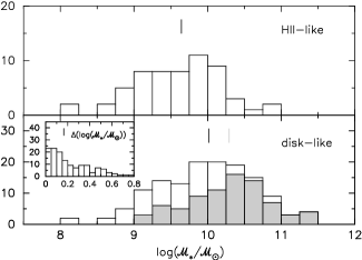
The median (mean) error in the determination of the stellar mass is 0.16dex (0.22dex), thus more than half of the galaxies have their stellar masses determined within a factor of 2 or better. These uncertainties are typical in this kind of studies based on broad-band photometry (e.g., Bell & de Jong, 2001; Papovich et al., 2001; Kauffmann et al., 2002). Mass errors are higher for galaxies with large burst strengths, since their global mass-to-light ratios are more affected by the young stellar population. Note that the $K$-band mass-to-light ratio of the young stellar population is strongly age-dependent, changing by a factor $\sim 15$ for ages from 1 to $10\,$Myr.

Fig. 13 splits the disk-like and HII-like spectroscopic types in sub-classes (cf. Paper I). This figure shows a clear trend from SBN objects to BCDs. The latter turn out to be the less massive objects, with an average mass of only $\sim 8\cdot 10^{8}\,\mathcal{M}_{\odot}$. Notice also that the DANS have quite a broad mass range.

There is also a trend in mass according to Hubble type. On average, the most massive objects are those presenting clear signs of interaction ($4\cdot 10^{10}\mathcal{M}_{\odot}$), followed by the S0s and the spirals, from early to late. Average stellar masses range from $2\cdot 10^{10}\mathcal{M}_{\odot}$ for lenticulars to $1\cdot 10^{10}\mathcal{M}_{\odot}$ for Sc$+$ and $4\cdot 10^{9}\mathcal{M}_{\odot}$ for irregulars.

Figure 13: Distributions of the total stellar masses (left) and specific SFR (right, in units of 10^-11 yr^-1) of the UCM objects for each one of the spectroscopic types. Median values are shown.

Figure 14: Relationship between the HI mass and the total stellar mass for the UCM galaxies. The best linear fit is also plotted. The equation of this line is $\log(\mathcal{M}_{\rm HI}/\mathcal{M}_{*})=(6.1\pm 1.1)-(0.67\pm 0.11)\cdot\log(\mathcal{M}_{*})$. The fit for the results obtained using the CALZ00  extinction recipe is very similar, $\log(\mathcal{M}_{HI}/\mathcal{M}_{*})=(6.17\pm 0.96)+(-0.67\pm 0.09)\cdot\log(\mathcal{M}_{*})$

In Fig. 14 we compare the relative gas content of the UCM Survey galaxies (the mass of neutral hydrogen normalized with the total stellar mass) vs. $\mathcal{M}_{*}$. Clearly, higher mass galaxies have lower gas fractions. This suggests that these objects may have exhausted most of their gas and turned it into stars. Less massive objects have a larger gas reservoir, in relative terms, and thus have more raw material available for current/future star formation. Obviously, the molecular phase has not been considered here, but our arguments should remain valid provided that the H₂/HI ratio does not vary wildly. Given that low-mass galaxies also present high values of the specific SFR (SFR per unit mass, see Section 6), this appears to be a direct consequence of the well-known Schmidt Law (Schmidt, 1959).

Using the dynamical masses calculated by Pisano et al. (2001) for 11 UCM galaxies we can calculate the ratio of stellar to dynamical masses for this small sample. We find an average value of $\mathcal{M}_{*}=(0.19\pm 0.14)\mathcal{M}_{\rm dyn}$, with values ranging from 0.02 to 0.60. These figures are well within the range of mass ratios found by other authors (e.g., Boselli et al., 1997; Brinchmann & Ellis, 2000), albeit for a very small number of galaxies.

Figure 15: Oxygen abundance vs. total stellar mass. The data is fitted with the line $12+\log({\rm O/H})=(6.409\pm 0.245)+(0.223\pm 0.025)\cdot\log(\mathcal{M}_{*})$. The standard deviation of the fit is $\sigma=0.213$. When using the CALZ00  extinction recipe, a very similar fit is found $12+\log({\rm O/H})=(6.024\pm 0.281)+(0.257\pm 0.028)\cdot\log(\mathcal{M}_{*})$.

Finally, figure 15 shows the correlation between the total stellar mass and the oxygen abundance of the UCM galaxies. The abundances have been calculated with the $\rm{[NII]}\lambda 6584/\rm H\alpha$ and $\rm{[OIII]}\lambda 5007$ ratios using the relations given by Melbourne & Salzer (2002) and presented elsewhere (Zamorano et al., 2002). See also Aragón-Salamanca et al. (2002). A clear stellar mass–metallicity relation is found. More massive galaxies have higher metal abundances, as expected. Larger stellar masses imply higher chemical enrichment of the interstellar medium.

6 Specific SFR and star-formation efficiency

Table 3: Median values and quartiles for total mass and specific star formation rate of the UCM Survey galaxies.

		$\log(\mathcal{M}_{*}/\mathcal{M}_{\odot})$				$\log(SFR/\mathcal{M}_{*})$
BC99		INST		CONS		INST		CONS
SALP	CF00	9.93	${}^{+0.57}_{-0.45}$	10.35	${}^{+0.35}_{-0.58}$	2.47	${}^{+0.32}_{-0.43}$	2.31	${}^{+0.36}_{-0.44}$
	CALZ00	10.00	${}^{+0.46}_{-0.38}$	10.23	${}^{+0.45}_{-0.45}$	2.46	${}^{+0.31}_{-0.40}$	2.28	${}^{+0.40}_{-0.28}$
SCA	CF00	9.79	${}^{+0.48}_{-0.38}$	10.11	${}^{+0.37}_{-0.50}$	2.62	${}^{+0.33}_{-0.35}$	2.48	${}^{+0.44}_{-0.40}$
	CALZ00	9.89	${}^{+0.41}_{-0.40}$	10.01	${}^{+0.41}_{-0.44}$	2.55	${}^{+0.32}_{-0.28}$	2.50	${}^{+0.39}_{-0.30}$
MSCA	CF00	9.63	${}^{+0.49}_{-0.43}$	9.71	${}^{+0.51}_{-0.56}$	2.81	${}^{+0.33}_{-0.37}$	2.77	${}^{+0.44}_{-0.40}$
	CALZ00	9.72	${}^{+0.42}_{-0.40}$	9.77	${}^{+0.51}_{-0.51}$	2.72	${}^{+0.32}_{-0.29}$	2.69	${}^{+0.45}_{-0.30}$
SB99		INST		CONS		INST		CONS
SALP	CF00	10.02	${}^{+0.42}_{-0.51}$	10.41	${}^{+0.32}_{-0.60}$	2.48	${}^{+0.25}_{-0.39}$	2.21	${}^{+0.43}_{-0.37}$
	CALZ00	10.11	${}^{+0.40}_{-0.59}$	10.29	${}^{+0.40}_{-0.52}$	2.40	${}^{+0.28}_{-0.32}$	2.30	${}^{+0.43}_{-0.32}$
Best Fit	objects	log($\mathcal{M}_{*}$/$\mathcal{M}$⊙)				log(SFR/$\mathcal{M}_{*}$)
total	154	9.86	${}^{+0.48}_{-0.54}$			2.60	${}^{+0.27}_{-0.36}$
disk$-$like	95	10.16	${}^{+0.33}_{-0.44}$			2.44	${}^{+0.24}_{-0.26}$
HII$-$like	59	9.43	${}^{+0.38}_{-0.43}$			2.78	${}^{+0.52}_{-0.16}$
SBN	73	10.27	${}^{+0.31}_{-0.24}$			2.42	${}^{+0.26}_{-0.26}$
DANS	22	9.37	${}^{+0.18}_{-0.09}$			2.57	${}^{+0.11}_{-0.18}$
HIIH	40	9.58	${}^{+0.35}_{-0.27}$			2.71	${}^{+0.35}_{-0.14}$
DHIIH	12	8.89	${}^{+0.36}_{-0.29}$			2.85	${}^{+0.57}_{-0.18}$
BCD	7	8.45	${}^{+0.18}_{-0.15}$			3.59	${}^{+0.23}_{-0.41}$

Table 3: Median values and quartiles are shown for the total stellar mass (in solar units) and specific SFR (in $10^{-11}\,\mathrm{y}r^{-1}$). All the possible model input choices are considered. The last rows give the median values and quartiles of the best fits for each galaxy.

Figure 16: Specific SFR (in $10^{-11}\,$yr^-1) vs. total stellar mass. The panel on the left corresponds to different comparison galaxy samples (see text for details). The panel on the right corresponds to the UCM galaxies. Symbols refer to the different spectroscopic types. Also, filled symbols correspond to disk-like galaxies and open ones to HII-like ones (see Gallego et al., 1996, and Section 2.3 of Paper I).

In Paper I  we found that most of the UCM galaxies were best fitted using an instantaneous recent star formation event rather than a constant SFR overimposed on a normal relaxed spiral galaxy. In this scenario, the “current SFR” is meaningless since the burst might have occurred a few Myr ago and now the SFR associated with the burst is zero. In Alonso-Herrero et al. (1996), Guzmán et al. (1997) and GdP00, an effective SFR was introduced. This effective SFR is equivalent to the rate we would derive if a galaxy was forming stars at a constant rate during the time it shows detectable $\rm H\alpha$ emission (i.e., $EW(\rm H\alpha)>20\,$Å for the UCM Survey), producing a young population of the same mass as the one derived by our models.

In this sense, we can define the ratio between ratio between the $\rm H\alpha$ luminosity and the effective current SFR. Our intention is not to provide a universal conversion between $\rm H\alpha$ luminosity and current SFR but to be able to compare the results from our sample to those available in the literature. Following the same procedure explained in Alonso-Herrero et al. (1996) we have adopted

$${\rm SFR}=\frac{\mathrm{L}_{H_{\alpha}}}{0.7\cdot 10^{40}\rm erg\,s^{-1}}\,\mathcal{M}_{\odot}\,\rm{yr^{-1}}$$ (2)

This ratio has been obtained using the SB99  models for instantaneous SFR, Salpeter IMF and the CF00  extinction recipe.

Using this expression, we have calculated the current SFR for the UCM galaxies from their $L({{\rm H}\alpha})$ (Gallego et al., 1996) and also the specific SFR (SFR$/\mathcal{M}_{*}$), defined as the current star formation rate per unit stellar mass (see in Table LABEL:allres).

Fig. 13 shows the distribution of specific star formation rates for the UCM sample divided by spectroscopic type. This plot confirms the result found by GdP00: HII-like galaxies show larger specific SFRs than disk-like objects. The difference between the median values for the most extreme cases, SBN and BCD, is well over an order of magnitude.

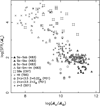
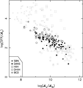
Finally, Fig. 16 shows the relationship between the specific SFR and the total stellar mass for the UCM Survey galaxies. We use different symbols for different spectroscopic types. Several comparison galaxy samples are also shown. (1) The sample of ‘normal’ disk galaxies with $\rm H\alpha$ and $B$-band luminosities given by Kennicutt (1983) and stellar mass-to-light ratios estimated by Faber & Gallagher (1979). (2) The starburst galaxies studied by Calzetti (1997). (3) The sample of HII-galaxies of Telles (1995), whose virial masses were converted to stellar masses using a 0.6dex offset (GdP00). (4) The sample of galaxies with $2<z<3.5$ analysed by Papovich et al. (2001). (5) The $z\sim 3$ Lyman-break galaxies studied by Shapley et al. (2001).

Figure 16 shows a clear segregation between spectroscopic types. Disk-like objects tend to be massive galaxies with lower values of the specific SFR. In general, they are experiencing a burst which is not very intense relatively to their total masses. Conversely, in HII-like galaxies the current/recent episode of star formation is, in relative terms, much more important. However, there is considerable overlap in specific SFRs and masses. The SBN objects represent the extreme case of low specific SFR and high stellar mass, while the BCDs and some DHIIH objects appear at the other extreme, experiencing a burst of star formation which is very strong for their low masses. The HIIH and DHIIH galaxies occupy the middle range (see also Fig.13).

We notice also that in this diagram the DANS galaxies show quite a large spread in properties. A number of them are placed in the region dominated by SBNs while others present masses and specific SFRs similar to HII-like galaxies. In addition, there is a relatively large group of these objects with stellar masses similar to HII galaxies but weaker SFR$/\mathcal{M}_{*}$. When fitting the observational data for the DANS galaxies with our models we noticed that all the massive DANS systems present an extinction best described by the CF00  recipe while the rest are best fitted with the CALZ00  law (using, in both cases, a Salpeter IMF and the SB99  code). This could indicate that the DANS objects constitute a heterogeneous group with a mixture of stellar population and star formation properties.

Comparing both panels in figure 16 it is clear that the UCM galaxies span a broad range in properties between the galaxies dominated by strong (in relative terms) current/recent star formation (e.g., extreme dwarf HII galaxies) and ‘normal’ spirals. We notice that the starburst galaxies studied by Calzetti (1997) appear outside the general trend delineated by the rest of the galaxies. Although their stellar masses are similar to those of the UCM galaxies, their specific SFRs are much higher, indicating that they are experiencing extremely strong bursts of star formation. Since these galaxies were selected by their strong starbursts, this result is not surprising, but it is important to remember that these are extreme objects and thus not representative of the general star-forming galaxy population. Finally, it is interesting that, in this diagram, the $z\sim 3$ Lyman-break galaxies studied by Shapley et al. (2001) seem to have very similar properties to the UCM galaxies. Indeed, their stellar masses and specific SFRs cover similar ranges. It is clear that by $z\sim 3$ these systems have already built relatively large stellar systems, and that their star formation is similar to what is found in present-day ‘normal’ galaxies. These objects are clearly not experiencing the kind of violent episode of star formation present in the most extreme local starbursts: they are, in this sense, ‘typical’ galaxies.

7 Summary and conclusions

In this paper we have analysed the youngest stellar population of the sample of local star-forming galaxies in the UCM Survey. The youngest stars are responsible for the heating of the gas that is producing the emission-line spectrum, and in particular, the $\rm H\alpha$ line used to detect these objects. We have utilized the entire dataset available for the UCM sample, which includes optical and nIR photometry and optical spectroscopy, and population synthesis modelling to characterise these galaxies in terms of their stellar populations and star-formation histories. Our technique takes into account the observational uncertainties and considers individual star formation histories for each galaxy. The procedure and the observations used here were presented in the first paper of this series (Pérez-González et al., 2002b).

In this paper, the second of the series, we have presented derived burst strengths, ages and metallicities of the most recent star-forming event for each one of the UCM galaxies. Our method also allowed us to derive several global properties of the galaxies, such as the total stellar mass and the star formation rate. Our main results are:

• An ‘average’ UCM galaxy experienced, about $5\,$Myr ago, an instantaneous burst of star formation involving $\sim 5$% of the total stellar mass. Ages range from 1 to 10 Myr and burst strengths from $\sim 0.1$% to $\sim 100$%. Our method does not yield robust metallicity values.

• As argued in Pérez-González et al. (2002b), the extinction plays a key role. The derived intensity of the star formation event is highly dependent on this parameter, with the most violent starbursts being strongly attenuated by extinction. The detection of star-forming objects is also hindered by extinction, especially for very young bursts which may still be embedded in a dense dusty cloud. Moreover, since the nebular emission falls off rapidly after 10 Myr (and thus the EW of $\mathrm{H}\alpha$) for an instantaneous burst, galaxies with newly-formed stars older than this age will not be detected by our survey.

• Even for burst strengths as low as 1%, the young population emits an important fraction of the total luminosity at optical wavelengths. Thus, a correlation is expected between optical colours such as $B-r$ and the burst strength. This correlation is very clear for galaxies with low extinction. However, high-extinction galaxies do not show such correlation, probably because different extinctions would change the optical colours by different amounts, hiding any underlying trend. Nevertheless, a lower limit of the burst strength can be derived from $B-r$.

• For a typical UCM galaxy with $b=1$%, the newly-formed stars contribute $\sim$10% to the total $K$-band luminosity. For a larger burst strength of 10%, the contribution rises to 50% (Pérez-González et al., 2002b). Caution is thus needed when applying a constant mass-to-light ratio to calculate stellar masses, even in the $K$ band. For galaxies with strong star formation, the $M/L_{K}$ ratio can vary by a factor of a few.

• With that in mind, in this paper we have taken into account the derived contribution to the $K$ light from young and old stars when estimating reliable mass-to-light ratios for each galaxy. Typical internal uncertainties are $\sim 0.2$dex. These mass-to-light ratios have been used to estimate stellar masses for each UCM galaxy. We find no clear correlation between the derived mass-to-light ratios and the galaxy colours or luminosities. This agrees with the findings of Kauffmann et al. (2002) for galaxies fainter than $L^{*}$.

• An ‘average’ UCM galaxy has a total stellar mass of $\sim 10^{10}\,\mathcal{M}_{\odot}$, i.e., about a factor of $7$–$10$ lower than an $L_{K}^{*}$ galaxy (Cole et al., 2001). The range of stellar masses in our sample is quite broad, from massive $10^{11}\mathcal{M}_{\odot}$ (i.e., $\sim L^{*}$) galaxies to $10^{8}\mathcal{M}_{\odot}$ dwarfs. However, our evidence indicates that star-formation in the local universe is dominated by galaxies considerably less massive than $L^{*}$.

• We have divided the star-forming galaxies in the UCM sample into two broad spectroscopic classes, disk-like and HII-like. Although this classification is spectroscopic in nature, most of the disk-like galaxies show disk/spiral morphologies, while the HII-like have, in general, a more compact appearance. The disk-like galaxies are mainly massive galaxies (mass greater than $10^{10}\mathcal{M}_{\odot}$) while the HII-like are dominated by objects with a lower mass. The HII-like galaxies have, comparatively, higher gas fractions (relative to their total stellar mass). This gas is being transformed into stars with a higher efficiency than in disk-like galaxies, resulting in a higher specific star formation rate (SFR per unit stellar mass).

• The UCM galaxies span a broad range in properties between those of galaxies completely dominated by current/recent star formation (e.g., extreme dwarf HII galaxies) and those of ‘normal’ spirals. Interestingly, the $z\sim 3$ Lyman-break galaxies seem to have very similar properties to the UCM galaxies, indicating that by $z\sim 3$ these systems have already built relatively large stellar systems, and that their star formation is similar to what is found in present-day ‘normal’ galaxies.

In this paper we have only considered the integrated properties of the UCM galaxies. Future work will improve our understanding of these galaxies by carrying out a similar study of their spatially-resolved stellar populations and star-formation properties. A key role will be played by $\rm H\alpha$ CCD images recently obtained for the UCM galaxies (Pérez-González et al., 2002c).

APPENDIX: Comments on individual objects

We comment here on some interesting objects found when inspecting Fig. 16:

• Two galaxies classified as DHIIH (UCM1302$+$2853 and UCM0047$-$0213), appear in the zone dominated by SBN or extreme HIIH galaxies [2 open circles with $\log(\mathcal{M}_{*}/\mathcal{M}_{\odot})\simeq 10.3$]. These objects have low $\rm H\alpha$ emission but intermediate $K$-band luminosities and masses. The ages of their young populations are rather high (over $8\,$Myr) and thus we may be observing a dying burst.

• UCM2319$+$2234 was classified as SBN but our models indicate that it is a low-mass almost pure starburst. Note that we need to use the CALZ00  extinction recipe to achieve a reasonable fit for this object. The high value of $b$ makes it extremely blue ($B-r=0.25\pm 0.06$), and gives it a very large ultraviolet excess (Takase & Miyauchi-Isobe, 1990).

• UCM2320$+$2428 (filled star at the bottom-right corner of Fig. 16) is an edge-on massive galaxy with a very low specific star formation and was classified as DANS. Its luminosity is large in all the observed bands ($M_{K}=-25.48\pm 0.05$) but the probable nuclear burst is very extincted [$E(B-V)=1.30$]. This high reddening is partially responsible for its spectroscopic classification.

• The most massive objects are grand-design spirals (e.g., UCM2238$+$2308, UCM2316$+$2457, UCM2324$+$2448 and UCM2325+2208) or distorted galaxies with clear signs of interactions (e.g., UCM0000$+$2140, UCM1537$+$2506N and UCM1653$+$2644).

• Distorted objects also appear among galaxies with high SFR/$\mathcal{M}_{*}$ (e.g., UCM0056$+$0044 and UCM2250$+$2427).

References

- Abraham et al. (1999) Abraham R. G., Ellis R. S., Fabian A. C., Tanvir N. R., Glazebrook K., 1999, MNRAS, 303, 641
- Alonso et al. (1999) Alonso O., García-Dabó C. E., Zamorano J., Gallego J., Rego M., 1999, ApJS, 122, 415
- Alonso-Herrero et al. (1996) Alonso-Herrero A., Aragón-Salamanca A., Zamorano J., Rego M., 1996, MNRAS, 278, 417
- Aragón-Salamanca et al. (2002) Aragón-Salamanca A., Alonso-Herrero A., Gallego J., García-Dabó C. E., Gil de Paz A., Pérez-González P., Zamorano J., 2002, AJ, submitted
- Bell & de Jong (2000) Bell E. F., de Jong R. S., 2000, MNRAS, 312, 497
- Bell & de Jong (2001) Bell E. F., de Jong R. S., 2001, ApJ, 550, 212
- Bolzonella et al. (2000) Bolzonella M., Miralles J.-M., Pelló R., 2000, A&A, 363, 476
- Boselli et al. (1997) Boselli A., Gavazzi G., Lequeux J., Buat V., Casoli F., Dickey J., Donas J., 1997, A&A, 327, 522
- Brinchmann & Ellis (2000) Brinchmann J., Ellis R. S., 2000, ApJL, 536, L77
- Calzetti (1997) Calzetti D., 1997, AJ, 113, 162
- Calzetti et al. (2000) Calzetti D., Armus L., Bohlin R. C., Kinney A. L., Koornneef J., Storchi-Bergmann T., 2000, ApJ, 533, 682
- Charlot & Fall (2000) Charlot S. ., Fall S. M., 2000, ApJ, 539, 718
- Cohen et al. (1999) Cohen J. G., Blandford R., Hogg D. W., Pahre M. A., Shopbell P. L., 1999, ApJ, 512, 30
- Cole et al. (2001) Cole S., Norberg P., Baugh C. M., Frenk C. S., Bland-Hawthorn J., Bridges T., Cannon R., Colless M., et al. 2001, MNRAS, 326, 255
- Cowie et al. (1996) Cowie L. L., Songaila A., Hu E. M., Cohen J. G., 1996, AJ, 112, 839
- Davidge (1992) Davidge T. J., 1992, AJ, 103, 1512
- de Jong (1996) de Jong R. S., 1996, A&A, 313, 377
- de Jong & van der Kruit (1994) de Jong R. S., van der Kruit P. C., 1994, A&AS, 106, 451
- Drory et al. (2001) Drory N., Bender R., Snigula J., Feulner G., Hopp U., Maraston C., Hill G. J., de Oliveira C. M., 2001, ApJL, 562, L111
- Faber & Gallagher (1979) Faber S. M., Gallagher J. S., 1979, ARA&A, 17, 135
- Fioc & Rocca-Volmerange (1999) Fioc M., Rocca-Volmerange B., 1999, A&A, 351, 869
- Fukugita et al. (1995) Fukugita M., Shimasaku K., Ichikawa T., 1995, PASP, 107, 945
- Gallego (1995) Gallego J., 1995, PhD thesis, Universidad Complutense de Madrid
- Gallego et al. (1996) Gallego J., Zamorano J., Rego M., Alonso O., Vitores A. G., 1996, A&AS, 120, 323
- Gil de Paz et al. (2000a) Gil de Paz A., Aragón-Salamanca A., Gallego J., Alonso-Herrero A., Zamorano J., Kauffmann G., 2000a, MNRAS, 316, 357
- Gil de Paz & Madore (2002) Gil de Paz A., Madore B. F., 2002, AJ, 123, 1864
- Gil de Paz et al. (2000b) Gil de Paz A., Zamorano J., Gallego J., 2000b, A&A, 361, 465
- Gil de Paz et al. (2000c) Gil de Paz A., Zamorano J., Gallego J., Domínguez F. D., 2000c, A&AS, 145, 377
- Gordon et al. (1997) Gordon K. D., Calzetti D., Witt A. N., 1997, ApJ, 487, 625
- Graham (2002) Graham A. W., 2002, MNRAS, 334, 721
- Guzmán et al. (1997) Guzmán R., Gallego J., Koo D. C., Phillips A. C., Lowenthal J. D., Faber S. M., Illingworth G. D., Vogt N. P., 1997, ApJ, 489, 559
- Huchtmeier & Richter (1989) Huchtmeier W. K., Richter O.-G., 1989, A General Catalog of HI Observations of Galaxies. The Reference Catalog. (A General Catalog of HI Observations of Galaxies. The Reference Catalog, XIX, 350 pp. 8 figs.. Springer-Verlag Berlin Heidelberg New York)
- Jarrett et al. (2000) Jarrett T. H., Chester T., Cutri R., Schneider S., Skrutskie M., Huchra J. P., 2000, AJ, 119, 2498
- Kauffmann et al. (2002) Kauffmann G., Heckman T. M., White S. D. M., Charlot S., Tremonti C., Peng E. W., Seibert M., Bernardi M., Brinkmann J., Castander F., Csabai I., Fukugita M., Ivezic Z., Munn J., Nichol R., Thakar A., Weinberg D., 2002, MNRAS (submitted), astro-ph/0204055
- Kennicutt (1983) Kennicutt R. C., 1983, ApJ, 272, 54
- Kennicutt (1992) Kennicutt R. C., 1992, ApJ, 388, 310
- Kennicutt (1998a) Kennicutt R. C., 1998a, ARA&A, 36, 189
- Kennicutt (1998b) Kennicutt R. C., 1998b, ApJ, 498, 541
- Kochanek et al. (2001) Kochanek C. S., Pahre M. A., Falco E. E., Huchra J. P., Mader J., Jarrett T. H., Chester T., Cutri R., Schneider S. E., 2001, ApJ, 560, 566
- Krüger et al. (1995) Krüger H., Fritze-v. Alvensleben U., Loose H.-H., 1995, A&A, 303, 41
- Kunth & Östlin (2000) Kunth D., Östlin G., 2000, A&AR, 10, 1
- Leitherer et al. (1999) Leitherer C., Schaerer D., Goldader J. D., Delgado R. M. G. ., Robert C., Kune D. F., de Mello D. . F., Devost D., Heckman T. M., 1999, ApJS, 123, 3
- Loveday (2000) Loveday J., 2000, MNRAS, 312, 557
- Melbourne & Salzer (2002) Melbourne J., Salzer J. J., 2002, AJ, 123, 2302
- Miller & Scalo (1979) Miller G. E., Scalo J. M., 1979, ApJS, 41, 513
- Moriondo et al. (1998) Moriondo G., Giovanardi C., Hunt L. K., 1998, A&A, 339, 409
- Papovich et al. (2001) Papovich C., Dickinson M., Ferguson H. C., 2001, ApJ, 559, 620
- Pérez-González et al. (2001) Pérez-González P. G., Gallego J., Zamorano J., Gil de Paz A., 2001, A&A, 365, 370
- Pérez-González et al. (2002a) Pérez-González P. G., Gil de Paz A., Zamorano J., Gallego J., 2002a, ApJ, in preparation
- Pérez-González et al. (2002b) Pérez-González P. G., Gil de Paz A., Zamorano J., Gallego J., Alonso-Herrero A., Aragón-Salamanca A., 2002b, MNRAS, in press, astro-ph/0209396
- Pérez-González et al. (2002c) Pérez-González P. G., Zamorano J., Gallego J., Aragón-Salamanca A., Gil de Paz A., 2002c, ApJ, in preparation
- Pérez-González et al. (2000) Pérez-González P. G., Zamorano J., Gallego J., Gil de Paz A., 2000, A&AS, 141, 409
- Pisano et al. (2001) Pisano D. J., Kobulnicky H. A., Guzmán R., Gallego J. ., Bershady M. A., 2001, AJ, 122, 1194
- Rix & Rieke (1993) Rix H., Rieke M. J., 1993, ApJ, 418, 123
- Roberts (1975) Roberts M. S., 1975, Galaxies and the Universe (Sandage, A., Sandage, M., Kristian, J., Chicago, University of Chicago Press), p. 309
- Salpeter (1955) Salpeter E. E., 1955, ApJ, 121, 161
- Scalo (1986) Scalo J. M., 1986, Fundamentals of Cosmic Physics, 11, 1
- Schmidt (1959) Schmidt M., 1959, ApJ, 129, 243
- Shapley et al. (2001) Shapley A. E., Steidel C. C., Adelberger K. L., Dickinson M., Giavalisco M., Pettini M., 2001, ApJ, 562, 95
- Strateva et al. (2001) Strateva I., Ivezić Ž., Knapp G. R., Narayanan V. K., Strauss M. A., Gunn J. E., Lupton R. H., Schlegel D., Bahcall N. A., Brinkmann J., Brunner R. J., Budavári T. ., Csabai I. ., Castander F. J., Doi M., Fukugita M., Győry Z., Hamabe M., Hennessy G., Ichikawa T., Kunszt P. Z., Lamb D. Q., McKay T. A., Okamura S., Racusin J., Sekiguchi M., Schneider D. P., Shimasaku K., York D., 2001, AJ, 122, 1861
- Takase & Miyauchi-Isobe (1990) Takase B., Miyauchi-Isobe N., 1990, Publications of the National Astronomical Observatory of Japan, 1, 181
- Telles (1995) Telles J. E., 1995, PhD thesis, Cambridge University
- Vitores et al. (1996) Vitores A. G., Zamorano J., Rego M., Alonso O., Gallego J., 1996, A&AS, 118, 7
- Worthey (1994) Worthey G., 1994, ApJS, 95, 107
- Zamorano et al. (1996) Zamorano J., Gallego J., Rego M., Vitores A. G., Alonso O., 1996, ApJS, 105, 343
- Zamorano et al. (1994) Zamorano J., Rego M., Gallego J. G., Vitores A. G., González-Riestra R., Rodríguez-Caderot G., 1994, ApJS, 95, 387
- Zamorano et al. (2002) Zamorano et al. 2002, ApJ, in preparation