Stellar populations in local star-forming galaxies.
I.–Data and modelling procedure.

Abstract

We present an analysis of the integrated properties of the stellar populations in the Universidad Complutense de Madrid (UCM) Survey of $\mathrm{H}\alpha$-selected galaxies. In this paper, the first of a series, we describe in detail the techniques developed to model star-forming galaxies using a mixture of stellar populations, and taking into account the observational uncertainties. We assume a recent burst of star formation superimposed on a more evolved population. The effects of the nebular continuum, line emission and dust attenuation are taken into account. We also test different model assumptions including the choice of specific evolutionary synthesis model, initial mass function, star formation scenario and the treatment of dust extinction. Quantitative tests are applied to determine how well these models fit our multi-wavelength observations for the UCM sample. Our observations span the optical and near infrared, including both photometric and spectroscopic data. Our results indicate that extinction plays a key role in this kind of studies, revealing that low- and high-obscured objects may require very different extinction laws and must be treated differently. We also demonstrate that the UCM Survey galaxies are best described by a short burst of star formation occurring within a quiescent galaxy, rather than by continuous star formation. A detailed discussion on the inferred parameters, such as the age, burst strength, metallicity, star formation rate, extinction and total stellar mass for individual objects, is presented in paper II of this series.

1 Introduction

One of the main issues in today’s Astrophysics is how present day galaxies formed and how they have evolved over time. A considerable observational effort is being made to study galaxies from the earliest possible times to the present. Our knowledge of the faint galaxy populations over the $0<z<5$ range has experienced remarkable progress in a relatively short period of time (see the reviews by Ellis 1997 and Ferguson et al. 2000). One of the main aims of these studies is to find the progenitors of the local galaxy population. While the majority of local galaxies seem to fit reasonably well into the Hubble sequence, this morphological classification scheme breaks down at surprisingly low redshifts ($z\sim 0.3$-$0.5$; see Abraham & van den Bergh, 2002, and references therein). Moreover, new classes of distant objects have been discovered, such as Ultraluminous Infrared Galaxies, (Schmidt & Green, 1983), Extremely Red Objects, (Yan et al., 2000) as well as bright UV galaxies (Lyman Break Galaxies, LBGs, Steidel et al., 1996, 1999). The luminosity of these objects, both the reddest and the bluest, is mainly dominated by massive knots of newly-formed stars (starbursts), with different amounts of dust extinction.

A complementary approach to understand how present-day galaxies came into being is to study in detail the properties of local galaxies, and in particular their star-formation histories. In this respect, it is important to quantify the relative importance of the current episode of star formation in comparison to the underlying older stellar populations. Indeed, even in high redshift objects, stars formed before the currently-observed star formation episode must have been present in order to produce the observed metal and dust content. Examples of such high-$z$ objects include SCUBA sources (Hughes et al., 1998) and LBGs (see Calzetti 2001 and references therein). Moreover, an accurate determination of the total stellar mass in both local and distant galaxies is a necessary step towards understanding their formation (see, e.g., Pettini et al. 1998, 2001). Our group is actively working on the detailed study of galaxies in the Local Universe so that their properties can be compared with distant ones. The techniques developed and tested with local galaxies will have direct application in high-z studies.

The Universidad Complutense de Madrid (UCM) Survey was carried out in order to perform a comprehensive study of star-forming galaxies in the Local Universe (Zamorano et al. 1994, 1996; see also Alonso et al. 1999). This $\mathrm{H}\alpha$-selected galaxy sample has been extensively studied at optical and near infrared wavelengths (see next section). It has also been used to determine the local $\mathrm{H}\alpha$ luminosity function and star formation rate density (Gallego et al., 1995), providing a low-$z$ benchmark for intermediate and high-z studies (see, for example, Iwamuro et al., 2000; Moorwood et al., 2000; van der Werf et al., 2000; Tresse et al., 2001). Recently, the UCM Survey is being extended to higher redshifts (Pascual et al., 2001).

The present series of papers aims at determining the main properties of the stellar populations in the UCM Survey galaxies, accounting both for the newly-formed stars and the underlying evolved populations. We make use of the extensive multi-wavelength data available for the sample. A direct precursor of the current study was presented in Gil de Paz et al. (2000a, hereafter GdP00), where we characterized the stellar content of a smaller subsample of 67 UCM galaxies, constraining their ages, metallicities and relative strength of the current star-formation episode. A sophisticated statistical technique was developed by GdP00 to compare measurements and model predictions. We now present results for virtually all the UCM galaxies, increasing the sample by a factor of 2.5. We have also included additional photometry in the $B$-band (Pérez-González et al., 2000), and use a more elaborated spectral synthesis method.

The present paper will focus on the modelling technique and the observational data used to test it. We will discuss the model input parameters that best describe the observed properties of the UCM galaxies, including the initial mass function (IMF), star formation scenarios and extinction prescriptions. We will also study in detail how well our modelling techniques are able to reproduce the observations. In Pérez-González et al. (2002b, Paper II  hereafter), the second paper of the series, we will present the derived properties of the UCM galaxies using these data and techniques. Paper II will discuss the young and newly-formed stars in the galaxies, together with the underlying population of evolved stars, the total stellar masses, etc.

This paper is structured as follows: section 2 introduces the sample, the observations and the data measurements. Section 3 describes our modelling techniques, including the main features of the stellar and nebular emission models, the star formation scenarios and the extinction prescriptions. Section 4 discusses the goodness of the fits and possible correlations with the input data. Finally, Section 5 summarizes our conclusions. Throughout this paper we use a cosmology with $\mathrm{H}_{0}=70$ km s^-1 Mpc^-1, $\Omega_{\mathrm{M}}$=0.3 and $\Lambda$=0.7.

2 Data

2.1 The sample

The UCM Survey galaxy sample contains 191 galaxies selected by their $\mathrm{H}\alpha$ emission at an average redshift of 0.026 (Zamorano et al., 1994, 1996; Gallego et al., 1996). Out of these galaxies, 15 were classified as active galactic nuclei (AGN, including Seyfert 1, Seyfert 2 and LINER types) by Gallego et al. (1996), and will be excluded from the present study. The rest are star-forming galaxies. Eleven of these were observed only in two photometric bands, and comparison with the models has not been attempted. Thus, the sample studied here contains 163 galaxies, i.e., 94% of all the star-forming galaxies in the complete UCM sample. This represents a factor of 2.5 increase over the sample studied by GdP00.

The sample contains low excitation, high metallicity objects (often with bright and dusty starbursts) and high excitation, low metallicity ones with blue star-forming knots which may sometimes dominate the optical luminosity of the whole galaxy, as in the case of Blue Compact Dwarfs—BCDs. These two global spectroscopic types will be called disk-like and HII-like galaxies, respectively. There is also a large spectrum of sizes and masses (from grand-design spirals to dwarfs), luminosities, emission-line equivalent widths and star formation rates (SFRs). The data required in the present work are available for 94% of the entire UCM sample (excluding AGN). The galaxies studied here are thus a virtually complete sample, with no biases against any of the previously mentioned properties.

The dataset used in this work comprises a great deal of observations, both photometric and spectroscopic. Most of them have already been presented in previous papers. Only near infrared (nIR) data for the whole UCM Survey has not been described before. In the next subsections we will review all these data, with special emphasis on the nIR campaigns.

2.2 Imaging

2.2.1 Optical: $B$- and $r$-bands

Gunn $r$ and Johnson $B$ observations were obtained in several observing runs from 1989 to 2001 using 1-2 metre-class telescopes at the German-Spanish Observatory of Calar Alto (CAHA, Almería, Spain) and the Observatorio del Roque de los Muchachos (La Palma, Spain). The observing details as well as the reduction and calibration procedures can be found in Vitores et al. (1996a, b) for the $r$ data, and Pérez-González et al. (2000) and Pérez-González et al. (2001) for $B$. Briefly, the sample has average magnitudes of $m_{B}$=16.1$\pm$1.1 ($M_{B}=-19.2$) and $m_{r}=15.5\pm 1.0$ ($M_{r}=-19.8$), with a mean $B$-band effective radius of 2.8 kpc. Up to 65% of the sample galaxies are classified as Sb or later.

2.2.2 Near infrared: $J$- and $K$-bands

Near infrared observations for a small subsample of 67 galaxies were presented in GdP00. The whole sample of 191 galaxies has now been observed in the nIR.

A total number of 11 campaigns were necessary to complete the 191 objects. These runs were carried out from January 1996 to April 2002 in 1-2 metre-class telescopes: the 2.2m Telescope at Calar Alto Observatory (Almería, Spain), the 1m Telescope at UCO/Lick Observatory (California,USA) and the 2.3m Bok Telescope of the University of Arizona on Kitt Peak Observatory (Arizona, USA). Basic information on each observing run are given in Table 1. The filters used in these runs were $J$, $K$, $K_{s}$ and $K^{\prime}$. Standard reduction procedures in the nIR were applied, a description of which can be found in Aragón-Salamanca et al. (1993). Flux calibration was performed using standard stars from the lists of Elias et al. (1982); Hunt et al. (1998); Hawarden et al. (2001). For each photometric night, appropriate atmospheric extinction coefficients were derived and zero-points for each observing setup determined. Non-photometric data were calibrated using short exposures of the fields taken during photometric nights. The magnitudes of the 62 galaxies observed in $K^{\prime}$ were transformed into the standard $K$ system by applying the constant offset $K^{\prime}-K$=0.07 mag (Wainscoat & Cowie, 1992; Aragón-Salamanca et al., 1993). The correction from $K_{s}$ to $K$ is negligible (Persson et al., 1998).

Table 1: Log of the nIR observation for the UCM sample.

Telesc./Observ.	Dates	Chip	Plate scale	Conditions
(1)	(2)	(3)	(4)	(5)
Lick 1.0m	Jan 9-14 1996	NICMOS3 256x256	0.57	3 photometric nights
Lick 1.0m	May 4-7 1996	NICMOS3 256x256	0.57	2 photometric nights
Lick 1.0m	Jun 7-9 1996	NICMOS3 256x256	0.57	photometric
CAHA 2.2m	Aug 4-6 1996	NICMOS3 256x256	0.63	photometric
Bok 2.3m	Jan 10-17 1998	NICMOS3 256x256	0.60	2 photometric nights
Bok 2.3m	Nov 01-07 1998	NICMOS3 256x256	0.60	photometric
Bok 2.3m	Mar 20-23 1999	NICMOS3 256x256	0.60	photometric
Bok 2.3m	Sep 27-30 1999	NICMOS3 256x256	0.60	rainy
Bok 2.3m	Nov 07-09 2000	NICMOS3 256x256	0.60	photometric
Bok 2.3m	Nov 29- Dec 01 2001	NICMOS3 256x256	0.60	1 photometric night
Bok 2.3m	Mar 30- Apr 01 2002	NICMOS3 256x256	0.60	photometric

Table 1: Observing log for the nIR observations of the UCM Survey galaxies. Columns stand for: (1) Telescope name. (2) Date of the observation. (3) Detector used. (4) Scale of the chip in arcsec$\cdot$pixel^-1. (5) Weather conditions.

2.3 Long-slit optical spectroscopy

We use redshifts, $\mathrm{H\alpha+[NII]}$ equivalent widths ($EW$), $\mathrm{H\alpha/[NII]}$ and $\mathrm{H}\alpha/\mathrm{H}\beta$ intensity ratios, and spectroscopic types from Gallego et al. (1996). The $EW(\mathrm{H\alpha+[NII]})$ was transformed into $EW(\mathrm{H}\alpha)$ using the observed $\mathrm{H\alpha/[NII]}$ ratios when available. For the 20 galaxies without measured $\mathrm{[NII]/H\alpha}$ ratios we assumed average values for the relevant spectroscopic types. Errors for the $\mathrm{H}\alpha$ equivalent width are estimated to be $\simeq 20$%.

For 30 objects, the $\mathrm{H}\alpha/H\beta$ ratio was impossible to measure due to high extinction and/or to stellar absorption leading to the absence of detectable $\mathrm{H}\beta$ emission. In these cases, the average value of the 25% highest ratios for each spectroscopic type has been assumed. The rationale behind this assumption is that these galaxies must have high extinctions in order to completely obliterate the $\mathrm{H}\beta$ emission line.

The emission-line data was corrected for underlying stellar population absorption. Kurucz (1992) established that the $\mathrm{H}\alpha$ and $\mathrm{H}\beta$ equivalent widths are equal within a 30% uncertainty. Thus, we used a typical stellar absorption equivalent width for both $\mathrm{H}\alpha$ and $\mathrm{H}\beta$ of 3Å  (Trager et al. 1998; González Delgado et al. 1999).

Although described elsewhere (see Gallego et al. 1996 for details), we outline here the main properties of the different spectroscopic types that will be used later in the discussion and in Paper II:

SBN —Starburst Nuclei— Originally defined by Balzano (1983), they show high extinction values, with very low $\mathrm{[NII]/H\alpha}$ ratios and faint $\mathrm{[OIII]\lambda 5007}$ emission. Their $\mathrm{H}\alpha$ luminosities are always higher than $10^{8}\,L_{\sun}$.

DANS —Dwarf Amorphous Nuclear Starburst— Introduced by Salzer et al. (1989), they show very similar spectroscopic properties to SBN objects, but with $\mathrm{H}\alpha$ luminosities below $5\cdot 10^{7}\,L_{\sun}$.

HIIH —HII Hotspot— The HII Hotspot class shows similar $\mathrm{H}\alpha$ luminosities to those measured in SBN galaxies but with large $\mathrm{[OIII]\lambda 5007/H\beta}$ ratios, that is, higher ionization.

DHIIH —Dwarf HII Hotspot—- This is an HIIH subclass with identical spectroscopic properties but $\mathrm{H}\alpha$ luminosities lower than $5\cdot 10^{7}\,L_{\sun}$.

BCD —Blue Compact Dwarf— The lowest luminosity and highest ionization objects have been classified as Blue Compact Dwarf galaxies. They show in all cases $\mathrm{H}\alpha$ luminosities lower than $5\cdot 10^{7}\,L_{\sun}$ as well as large $\mathrm{[OIII]\lambda 5007/H\beta}$ and $\mathrm{H\alpha/[NII]\lambda 6584}$ line ratios and intense $\mathrm{[OII]\lambda 3727}$ emission.

All these spectroscopic classes are usually collapsed in two main categories: disk-like and HII-like galaxies (see Guzmán et al. 1997 and Gallego 1998). The disk-like class includes SBN and DANS spectroscopic types, whereas the HII-like includes HIIH, DHIIH and BCD galaxies.

2.4 Photometry analysis

Standard reduction procedures were applied to each photometric dataset. The sky level was measured using $\sim 30$ circular apertures of $\sim 100$ pixels² area placed at different positions around each object. The average of all the measurements and its standard deviation were used to determine the sky background and the related uncertainty.

In order to study the integrated properties of the galaxies, aperture photometry was obtained for each bandpass. Aiming at including the majority of the galaxy light, we used apertures with radii equal to three exponential disk scale lengths as determined in the $r$-band images (Vitores et al. 1996b). In the few cases when the $r$-band bulge-disk decomposition was not available, we used the radius of the 24 mag$\cdot$arcsec² isophote measured in the $B$-band ($r_{24}$, Pérez-González et al. 2001). We inspected each image visually and checked that these apertures were encompassing all the detectable galaxy flux, and that no artifacts were disturbing the data. In a few cases we slightly decreased or increased the aperture radius in order to ensure that the measured flux was as close as possible to the total flux. The photometric apertures were centred on the peak of the galaxy light in each band. We checked that the effect of possible misalignments between the light peaks in the different bands was always below the photometric uncertainty. We estimate that the size of this effect is always below 0.05 mag in $B$ and $r$ and 0.1 mag in $J$ and $K$.

Total $K$-band magnitudes were determined interactively as the average of the measurements inside the outer apertures where the curve of growth was flat. These fluxes were converted to absolute magnitudes and corrected for Galactic extinction using the maps published by Schlegel et al. (1998).

Since the model-fitting procedure (explained in Sect. 3.5) takes into account the observational errors, we took special care in their determination. The main sources of uncertainty are photon-counting errors (described by Poisson statistics), readout noise, flat-field errors (affecting mainly the sky determination), and photometric calibration uncertainties. For a given aperture, the uncertainty due to photon-counting errors and readout noise can be written as:

$$\sigma_{\mathrm{P}oisson}=\frac{\sqrt{\left(C_{\mathrm{g}al}+n_{\mathrm{g}al}\cdot C_{\mathrm{s}ky}\right)\cdot G+n_{\mathrm{g}al}\cdot RON^{2}}}{G}$$ (1)

where $C_{\mathrm{g}al}$ is the number of counts coming from the galaxy, $n_{\mathrm{g}al}$ the number of pixels inside the aperture, $C_{\mathrm{s}ky}$ the sky value in counts, and $G$ and $RON$ the gain and readout noise of the detector, measured in electrons/pixel and electrons, respectively.

The error in the total flux arising from the determination of the sky value is

$$\sigma_{\mathrm{s}kydet.}=\sigma_{\mathrm{s}ky}\cdot n_{\mathrm{g}al}$$ (2)

where $\sigma_{\mathrm{s}ky}$ is the standard deviation of the sky measurements mentioned before.

Expressing the previous uncertainties in magnitudes, we get

$$\Delta m_{\mathrm{i}mage}=1.0857\cdot\frac{\sqrt{\left(\sigma_{\mathrm{P}oisson}^{2}+\sigma_{\mathrm{s}kydet.}^{2}\right)}}{C_{\mathrm{g}al}\cdot\sqrt{N_{\mathrm{i}m}}}$$ (3)

where $N_{\mathrm{i}m}$ is the number of images of the same object, ranging from 1 in the optical filters to 20-24 in the nIR ones.

Finally, this quantity must be combined with the standard deviation of the photometric calibration ($\sigma_{\mathrm{z}ero-point}$) to obtain the total error in the magnitudes:

$$\Delta m_{T}=\sqrt{(\Delta m_{\mathrm{i}mage})^{2}+\sigma_{\mathrm{z}ero-point}^{2}}$$ (4)

Typical total errors are 0.04 mag in $B$, 0.03 mag in $r$ and 0.09 mag in $J$ and $K$.

Table 2: Photometric and spectroscopic data for the whole UCM sample.

UCM name	z	$m_{B}$	$m_{r}$	$m_{J}$	$m_{K}$	$EW(\mathrm{H}\alpha)$	$3d_{L}$ (kpc)	$\frac{F_{\mathrm{H}\alpha}}{F_{\mathrm{H}\beta}}$	$A_{V}^{\mathrm{G}al}$	MphT	SpT	$M_{K}$
(1)	(2)	(3)	(4)	(5)	(6)	(7)	(8)	(9)	(10)	(11)	(12)	(13)
0000$+$2140	0.0238	14.61$\pm$0.03	$-$	11.71$\pm$0.11	10.37$\pm$0.03	103$\pm$21	13.9	7.55	0.15	INTER	HIIH	$-$24.73
0003$+$2200	0.0224	17.19$\pm$0.02	16.30$\pm$0.04	14.65$\pm$0.15	13.53$\pm$0.08	38$\pm$ 8	9.9	5.02	0.23	Sc$+$	DANS	$-$21.47
0003$+$2215	0.0223	15.89$\pm$0.02	$-$	$-$	11.36$\pm$0.03	25$\pm$ 5	7.6	5.62	0.24	Sc$+$	SBN	$-$23.62
0003$+$1955	0.0278	14.11$\pm$0.13	$-$	$-$	$-$	294$\pm$59	6.7	4.61	0.12	$-$	Sy1	$-$
0005$+$1802	0.0187	16.40$\pm$0.13	$-$	$-$	12.27$\pm$0.04	13$\pm$ 3	6.4	3.62	0.12	Sb	SBN	$-$22.31
0006$+$2332	0.0159	14.95$\pm$0.05	$-$	12.69$\pm$0.05	11.90$\pm$0.06	58$\pm$12	8.4	4.58	0.31	Sb	HIIH	$-$22.37
0013$+$1942	0.0272	17.13$\pm$0.02	16.60$\pm$0.03	15.03$\pm$0.07	14.07$\pm$0.06	124$\pm$25	13.2	3.61	0.13	Sc$+$	HIIH	$-$21.34
0014$+$1829	0.0182	16.50$\pm$0.03	15.91$\pm$0.04	14.66$\pm$0.15	13.65$\pm$0.18	131$\pm$26	5.7	9.80	0.16	Sa	HIIH	$-$21.53
0014$+$1748	0.0182	14.83$\pm$0.05	14.01$\pm$0.14	11.86$\pm$0.11	10.82$\pm$0.16	86$\pm$17	39.7	5.74	0.13	SBb	SBN	$-$23.71
0015$+$2212	0.0198	16.85$\pm$0.02	16.04$\pm$0.08	14.30$\pm$0.07	13.29$\pm$0.04	120$\pm$24	8.5	3.32	0.23	Sa	HIIH	$-$21.56
0017$+$1942	0.0260	15.91$\pm$0.02	15.38$\pm$0.07	14.01$\pm$0.08	13.09$\pm$0.07	100$\pm$20	18.7	4.37	0.17	Sc$+$	HIIH	$-$22.29
0017$+$2148	0.0189	16.95$\pm$0.05	$-$	14.31$\pm$0.24	13.30$\pm$0.04	74$\pm$15	3.0	4.66	0.21	Sa	HIIH	$-$21.43
0018$+$2216	0.0169	16.95$\pm$0.02	16.15$\pm$0.03	14.22$\pm$0.07	13.39$\pm$0.05	15$\pm$ 3	5.7	2.86	0.23	Sb	DANS	$-$21.08
0018$+$2218	0.0220	15.97$\pm$0.02	$-$	12.17$\pm$0.14	11.12$\pm$0.20	16$\pm$ 3	10.8	9.39	0.22	Sb	SBN	$-$23.81
0019$+$2201	0.0191	16.80$\pm$0.02	15.82$\pm$0.04	13.96$\pm$0.04	12.96$\pm$0.05	33$\pm$ 7	10.4	3.70	0.21	Sb	DANS	$-$21.69
0022$+$2049	0.0185	15.86$\pm$0.05	14.65$\pm$0.03	12.46$\pm$0.08	11.24$\pm$0.05	76$\pm$15	10.2	6.28	0.30	Sb	HIIH	$-$23.42
0023$+$1908	0.0251	16.83$\pm$0.05	$-$	14.66$\pm$0.31	13.83$\pm$0.07	121$\pm$24	3.2	4.08	0.19	Sc$+$	HIIH	$-$21.39
0034$+$2119	0.0315	15.86$\pm$0.03	$-$	$-$	11.84$\pm$0.07	19$\pm$ 4	12.2	3.58	0.11	SBc$+$	SBN	$-$23.91
0037$+$2226	0.0195	14.65$\pm$0.05	$-$	12.44$\pm$0.13	11.53$\pm$0.03	45$\pm$ 9	7.7	4.19	0.13	SBc$+$	SBN	$-$23.23
0038$+$2259	0.0464	16.39$\pm$0.05	15.61$\pm$0.04	13.84$\pm$0.26	12.99$\pm$0.04	21$\pm$ 4	33.8	4.63	0.09	Sb	SBN	$-$23.60
0039$+$0054	0.0191	15.22$\pm$0.05	$-$	$-$	11.93$\pm$0.07	23$\pm$ 5	8.8	8.75	0.07	Sc$+$	SBN	$-$22.74
0040$+$0257	0.0367	16.98$\pm$0.05	16.85$\pm$0.04	$-$	14.41$\pm$0.08	119$\pm$24	12.5	4.14	0.09	Sb	DANS	$-$21.64
0040$+$2312	0.0254	15.69$\pm$0.03	$-$	12.15$\pm$0.14	11.07$\pm$0.03	28$\pm$ 6	12.9	8.55	0.12	Sc$+$	SBN	$-$24.22
0040$+$0220	0.0173	17.25$\pm$0.15	16.61$\pm$0.03	15.16$\pm$0.04	14.23$\pm$0.03	77$\pm$15	4.4	3.86	0.07	Sc$+$	DANS	$-$20.23
0040$-$0023	0.0142	13.76$\pm$0.03	$-$	11.15$\pm$0.10	10.35$\pm$0.07	18$\pm$ 4	10.8	9.20	0.06	Sc$+$	LINER	$-$23.60
0041$+$0134	0.0169	14.42$\pm$0.04	$-$	$-$	11.46$\pm$0.08	12$\pm$ 2	13.3	8.96	0.08	Sc$+$	SBN	$-$22.87
0043$+$0245	0.0180	17.34$\pm$0.05	$-$	$-$	14.30$\pm$0.08	34$\pm$ 7	2.2	5.07	0.07	Sc$+$	HIIH	$-$20.26
0043$-$0159	0.0161	13.01$\pm$0.05	$-$	10.79$\pm$0.01	9.70$\pm$0.07	60$\pm$12	9.8	8.03	0.09	Sc$+$	SBN	$-$24.53
0044$+$2246	0.0253	16.06$\pm$0.15	14.90$\pm$0.08	12.54$\pm$0.07	11.47$\pm$0.05	25$\pm$ 5	33.8	7.42	0.12	Sb	SBN	$-$23.78
0045$+$2206	0.0203	15.06$\pm$0.05	$-$	12.94$\pm$0.07	12.04$\pm$0.05	80$\pm$16	5.6	4.14	0.15	INTER	HIIH	$-$22.71
0047$+$2051	0.0577	16.98$\pm$0.05	16.14$\pm$0.03	$-$	13.13$\pm$0.03	73$\pm$15	20.0	4.60	0.10	Sc$+$	SBN	$-$23.96
0047$-$0213	0.0144	15.73$\pm$0.04	14.97$\pm$0.04	13.13$\pm$0.13	12.25$\pm$0.04	40$\pm$ 8	10.5	4.94	0.15	S0	DHIIH	$-$21.94
0047$+$2413	0.0347	15.88$\pm$0.05	14.81$\pm$0.03	12.74$\pm$0.05	11.63$\pm$0.05	61$\pm$12	31.4	5.13	0.20	Sa	SBN	$-$24.39
0047$+$2414	0.0347	15.22$\pm$0.05	$-$	12.66$\pm$0.18	11.69$\pm$0.03	78$\pm$16	10.1	4.69	0.20	Sc$+$	SBN	$-$24.28
0049$-$0006	0.0377	18.68$\pm$0.05	18.52$\pm$0.04	17.80$\pm$0.09	16.62$\pm$0.14	346$\pm$69	7.4	2.86	0.08	BCD	BCD	$-$19.50
0049$+$0017	0.0140	17.19$\pm$0.03	16.69$\pm$0.09	15.36$\pm$0.05	14.50$\pm$0.07	310$\pm$62	6.2	2.86	0.08	Sb	DHIIH	$-$19.42
0049$-$0045	0.0055	15.34$\pm$0.02	$-$	13.05$\pm$0.15	12.31$\pm$0.07	73$\pm$15	1.6	4.79	0.13	Sb	HIIH	$-$19.73
0050$+$0005	0.0346	16.54$\pm$0.03	16.03$\pm$0.03	$-$	13.68$\pm$0.07	94$\pm$19	13.1	4.50	0.08	Sa	HIIH	$-$22.31
0050$+$2114	0.0245	15.56$\pm$0.05	14.78$\pm$0.03	12.76$\pm$0.09	11.59$\pm$0.09	69$\pm$14	15.5	5.73	0.13	Sa	SBN	$-$23.59
0051$+$2430	0.0173	15.40$\pm$0.15	$-$	11.94$\pm$0.09	11.06$\pm$0.04	34$\pm$ 7	5.7	6.12	0.15	Sa	SBN	$-$23.34
0054$-$0133	0.0512	16.00$\pm$0.04	$-$	12.99$\pm$0.13	11.80$\pm$0.07	23$\pm$ 4	13.4	8.79	0.12	Sb	SBN	$-$25.02
0054$+$2337	0.0164	15.27$\pm$0.03	$-$	13.27$\pm$0.09	12.66$\pm$0.09	62$\pm$12	6.2	4.68	0.16	Sc$+$	HIIH	$-$21.67
0056$+$0044	0.0183	16.82$\pm$0.05	16.52$\pm$0.10	15.55$\pm$0.15	14.54$\pm$0.16	399$\pm$80	17.7	3.03	0.09	Irr	DHIIH	$-$20.04
0056$+$0043	0.0189	16.63$\pm$0.05	16.20$\pm$0.03	$-$	13.88$\pm$0.07	53$\pm$11	6.8	3.81	0.09	Sb	DHIIH	$-$20.77
0119$+$2156	0.0583	16.66$\pm$0.29	15.46$\pm$0.10	13.31$\pm$0.05	11.93$\pm$0.04	16$\pm$ 3	145.6	7.89	0.17	Sb	Sy2	$-$25.20
0121$+$2137	0.0345	16.02$\pm$0.05	15.47$\pm$0.06	13.85$\pm$0.08	12.90$\pm$0.07	66$\pm$13	33.8	4.86	0.22	Sc$+$	SBN	$-$23.05
0129$+$2109	0.0344	15.01$\pm$0.04	$-$	12.06$\pm$0.07	11.00$\pm$0.05	32$\pm$ 6	14.4	8.41	0.19	SBc$+$	LINER	$-$24.95
0134$+$2257	0.0353	16.03$\pm$0.05	$-$	12.76$\pm$0.13	11.73$\pm$0.03	26$\pm$ 5	10.6	4.91	0.37	Sb	SBN	$-$24.40
0135$+$2242	0.0363	17.16$\pm$0.05	16.26$\pm$0.03	14.40$\pm$0.04	13.42$\pm$0.05	46$\pm$ 9	14.4	6.69	0.40	S0	DANS	$-$22.74
0138$+$2216	0.0591	17.71$\pm$0.03	$-$	14.35$\pm$0.20	13.18$\pm$0.07	10$\pm$ 2	7.4	3.35	0.39	Sc$+$	$-$	$-$24.11
0141$+$2220	0.0174	16.36$\pm$0.05	15.91$\pm$0.03	13.72$\pm$0.04	12.66$\pm$0.02	37$\pm$ 7	9.0	4.68	0.30	Sa	DANS	$-$21.88
0142$+$2137	0.0362	15.35$\pm$0.05	14.25$\pm$0.05	$-$	11.19$\pm$0.04	29$\pm$ 6	48.3	3.83	0.34	SBb	Sy2	$-$24.98
0144$+$2519	0.0409	15.67$\pm$0.05	14.98$\pm$0.06	13.12$\pm$0.11	12.13$\pm$0.12	29$\pm$ 6	38.2	5.66	0.42	SBc$+$	SBN	$-$24.20
0147$+$2309	0.0194	16.88$\pm$0.05	15.99$\pm$0.04	14.56$\pm$0.05	13.62$\pm$0.06	118$\pm$24	10.8	4.34	0.32	Sa	HIIH	$-$21.05
0148$+$2124	0.0169	17.19$\pm$0.05	16.49$\pm$0.03	15.23$\pm$0.04	14.43$\pm$0.06	136$\pm$27	6.2	3.26	0.21	BCD	BCD	$-$20.00
0150$+$2032	0.0323	16.46$\pm$0.15	16.19$\pm$0.10	15.07$\pm$0.40	13.49$\pm$0.08	171$\pm$34	29.9	3.34	0.25	Sc$+$	HIIH	$-$22.42
0156$+$2410	0.0134	15.33$\pm$0.04	14.66$\pm$0.03	13.02$\pm$0.04	12.24$\pm$0.05	40$\pm$ 8	10.9	4.45	0.31	Sb	DANS	$-$21.70
0157$+$2413	0.0177	15.08$\pm$0.09	13.79$\pm$0.04	11.08$\pm$0.07	10.36$\pm$0.03	25$\pm$ 5	30.1	5.03	0.33	Sc$+$	Sy2	$-$24.16
0157$+$2102	0.0106	15.01$\pm$0.04	14.58$\pm$0.03	13.01$\pm$0.04	12.31$\pm$0.05	61$\pm$12	7.6	3.89	0.29	Sb	HIIH	$-$21.10
0159$+$2354	0.0170	17.34$\pm$0.05	16.36$\pm$0.03	14.50$\pm$0.04	13.59$\pm$0.05	63$\pm$13	6.6	4.18	0.33	Sb	HIIH	$-$20.86
0159$+$2326	0.0178	16.01$\pm$0.05	14.87$\pm$0.03	12.78$\pm$0.07	11.84$\pm$0.05	28$\pm$ 6	12.1	6.14	0.28	Sc$+$	DANS	$-$22.82
1246$+$2727	0.0199	15.84$\pm$0.21	$-$	13.82$\pm$0.35	12.92$\pm$0.09	67$\pm$13	6.7	4.90	0.04	Irr	HIIH	$-$21.85
1247$+$2701	0.0231	16.76$\pm$0.09	16.12$\pm$0.03	14.49$\pm$0.03	13.69$\pm$0.05	28$\pm$ 6	12.8	3.21	0.04	Sc$+$	DANS	$-$21.33

Table 2: continued

UCM name	z	$m_{B}$	$m_{r}$	$m_{J}$	$m_{K}$	$EW(\mathrm{H}\alpha)$	$3d_{L}$ (kpc)	$\frac{F_{\mathrm{H}\alpha}}{F_{\mathrm{H}\beta}}$	$A_{V}^{\mathrm{G}al}$	MphT	SpT	$M_{K}$
(1)	(2)	(3)	(4)	(5)	(6)	(7)	(8)	(9)	(10)	(11)	(12)	(13)
1248$+$2912	0.0217	15.09$\pm$0.17	$-$	$-$	11.55$\pm$0.07	29$\pm$ 6	8.0	3.99	0.06	SBb	SBN	$-$23.33
1253$+$2756	0.0165	16.09$\pm$0.02	15.41$\pm$0.03	13.99$\pm$0.05	13.12$\pm$0.04	114$\pm$23	6.0	2.86	0.03	Sa	HIIH	$-$21.59
1254$+$2740	0.0161	16.25$\pm$0.03	15.54$\pm$0.04	$-$	$-$	58$\pm$12	18.5	4.28	0.04	Sa	SBN	$-$
1254$+$2802	0.0253	16.91$\pm$0.02	15.88$\pm$0.03	13.91$\pm$0.03	12.84$\pm$0.04	14$\pm$ 3	14.7	8.78	0.04	Sc$+$	DANS	$-$22.44
1255$+$2819	0.0273	16.10$\pm$0.12	15.33$\pm$0.03	13.63$\pm$0.05	12.66$\pm$0.05	47$\pm$ 9	19.7	4.16	0.04	Sb	SBN	$-$23.10
1255$+$3125	0.0258	16.46$\pm$0.13	15.30$\pm$0.03	13.44$\pm$0.14	12.55$\pm$0.17	64$\pm$13	12.6	3.92	0.06	Sa	HIIH	$-$22.77
1255$+$2734	0.0234	16.97$\pm$0.02	16.15$\pm$0.03	$-$	13.33$\pm$0.06	99$\pm$20	10.6	5.44	0.04	Sc$+$	SBN	$-$21.74
1256$+$2717	0.0273	17.93$\pm$0.13	$-$	$-$	15.35$\pm$0.14	62$\pm$12	3.6	3.85	0.03	S0	DHIIH	$-$20.04
1256$+$2732	0.0245	15.95$\pm$0.18	15.37$\pm$0.04	13.90$\pm$0.05	12.90$\pm$0.07	79$\pm$16	31.0	4.71	0.05	INTER	SBN	$-$22.26
1256$+$2701	0.0247	16.66$\pm$0.09	16.27$\pm$0.07	14.70$\pm$0.10	13.68$\pm$0.11	109$\pm$22	32.5	3.46	0.03	Sc$+$	HIIH	$-$21.49
1256$+$2910	0.0279	16.21$\pm$0.08	15.28$\pm$0.03	13.45$\pm$0.03	12.52$\pm$0.04	25$\pm$ 5	19.5	8.66	0.03	Sb	SBN	$-$23.16
1256$+$2823	0.0315	16.14$\pm$0.10	15.30$\pm$0.03	13.67$\pm$0.10	12.50$\pm$0.14	76$\pm$15	16.9	4.82	0.04	Sb	SBN	$-$23.35
1256$+$2754	0.0172	15.43$\pm$0.07	14.90$\pm$0.03	13.18$\pm$0.05	12.25$\pm$0.05	49$\pm$10	14.5	4.12	0.04	Sa	SBN	$-$22.44
1256$+$2722	0.0287	17.21$\pm$0.09	16.21$\pm$0.04	$-$	12.84$\pm$0.06	26$\pm$ 5	14.3	5.10	0.04	Sc$+$	DANS	$-$22.66
1257$+$2808	0.0171	16.38$\pm$0.02	15.66$\pm$0.03	14.26$\pm$0.32	12.91$\pm$0.29	29$\pm$ 6	7.2	5.57	0.03	Sb	SBN	$-$21.48
1258$+$2754	0.0253	16.02$\pm$0.09	15.58$\pm$0.07	$-$	13.22$\pm$0.08	101$\pm$20	17.5	6.01	0.03	Sb	SBN	$-$22.06
1259$+$2934	0.0239	13.99$\pm$0.09	12.85$\pm$0.03	10.78$\pm$0.05	9.78$\pm$0.04	148$\pm$30	43.3	7.75	0.04	Sb	Sy2	$-$25.37
1259$+$3011	0.0307	16.25$\pm$0.09	15.40$\pm$0.03	13.56$\pm$0.13	12.57$\pm$0.14	22$\pm$ 4	36.5	3.50	0.04	Sa	SBN	$-$23.08
1259$+$2755	0.0240	15.57$\pm$0.04	14.61$\pm$0.03	13.08$\pm$0.12	11.97$\pm$0.13	44$\pm$ 9	17.2	5.22	0.03	Sa	SBN	$-$23.25
1300$+$2907	0.0219	17.27$\pm$0.09	16.86$\pm$0.03	$-$	14.75$\pm$0.10	94$\pm$19	9.7	5.10	0.04	Sa	HIIH	$-$20.16
1301$+$2904	0.0266	15.97$\pm$0.10	15.57$\pm$0.03	14.07$\pm$0.05	13.39$\pm$0.06	69$\pm$14	16.1	3.13	0.04	Sb	HIIH	$-$22.03
1302$+$2853	0.0237	16.50$\pm$0.02	15.99$\pm$0.03	14.26$\pm$0.14	13.43$\pm$0.19	40$\pm$ 8	10.1	4.07	0.04	Sb	DHIIH	$-$22.24
1302$+$3032	0.0342	16.66$\pm$0.07	$-$	14.85$\pm$0.45	13.95$\pm$0.07	49$\pm$10	6.2	4.09	0.04	Sa	HIIH	$-$21.97
1303$+$2908	0.0261	16.82$\pm$0.10	16.28$\pm$0.03	15.27$\pm$0.06	14.31$\pm$0.08	165$\pm$33	17.5	2.86	0.04	Irr	HIIH	$-$20.99
1304$+$2808	0.0210	16.02$\pm$0.11	15.03$\pm$0.03	13.37$\pm$0.13	12.03$\pm$0.14	24$\pm$ 5	18.9	2.86	0.04	Sb	SBN	$-$22.83
1304$+$2830	0.0217	18.62$\pm$0.04	18.09$\pm$0.03	$-$	15.43$\pm$0.09	56$\pm$11	4.7	3.57	0.04	BCD	DHIIH	$-$19.45
1304$+$2907	0.0159	15.16$\pm$0.24	14.61$\pm$0.08	$-$	12.55$\pm$0.10	8$\pm$ 2	28.6	8.96	0.04	Irr	$-$	$-$21.64
1304$+$2818	0.0244	15.88$\pm$0.02	15.06$\pm$0.03	13.58$\pm$0.06	12.50$\pm$0.08	80$\pm$16	18.5	2.97	0.05	Sc$+$	SBN	$-$22.72
1306$+$2938	0.0209	15.59$\pm$0.03	15.09$\pm$0.03	13.60$\pm$0.05	12.37$\pm$0.06	100$\pm$20	10.6	3.93	0.04	SBb	SBN	$-$22.73
1306$+$3111	0.0168	16.44$\pm$0.02	15.54$\pm$0.03	13.85$\pm$0.08	13.11$\pm$0.07	61$\pm$12	7.1	6.52	0.04	Sc$+$	DANS	$-$21.26
1307$+$2910	0.0187	14.25$\pm$0.03	13.22$\pm$0.05	11.59$\pm$0.35	10.33$\pm$0.29	25$\pm$ 5	37.7	4.70	0.03	SBb	SBN	$-$24.22
1308$+$2958	0.0212	15.36$\pm$0.02	14.53$\pm$0.04	12.71$\pm$0.08	11.94$\pm$0.15	21$\pm$ 4	27.1	5.63	0.04	Sc$+$	SBN	$-$22.89
1308$+$2950	0.0242	14.91$\pm$0.13	13.90$\pm$0.04	11.83$\pm$0.11	10.77$\pm$0.18	37$\pm$ 7	49.3	8.84	0.04	SBb	SBN	$-$24.36
1310$+$3027	0.0234	16.70$\pm$0.09	15.80$\pm$0.03	13.74$\pm$0.07	12.86$\pm$0.05	70$\pm$14	14.6	7.27	0.04	Sb	DANS	$-$22.33
1312$+$3040	0.0233	15.71$\pm$0.09	14.80$\pm$0.03	12.94$\pm$0.05	11.74$\pm$0.07	53$\pm$11	16.6	3.82	0.04	Sa	SBN	$-$23.36
1312$+$2954	0.0230	16.20$\pm$0.09	15.24$\pm$0.03	13.27$\pm$0.14	12.44$\pm$0.34	44$\pm$ 9	19.4	7.07	0.04	Sc$+$	SBN	$-$22.82
1313$+$2938	0.0380	16.93$\pm$0.09	16.56$\pm$0.03	15.45$\pm$0.06	14.67$\pm$0.07	311$\pm$62	8.9	2.86	0.03	Sa	HIIH	$-$21.74
1314$+$2827	0.0253	16.39$\pm$0.03	15.72$\pm$0.04	$-$	13.12$\pm$0.06	48$\pm$10	10.1	4.62	0.04	Sa	SBN	$-$22.30
1320$+$2727	0.0247	17.51$\pm$0.13	17.08$\pm$0.03	$-$	14.86$\pm$0.08	52$\pm$10	7.9	2.98	0.06	Sb	DHIIH	$-$20.39
1324$+$2926	0.0172	18.09$\pm$0.13	17.24$\pm$0.03	15.92$\pm$0.03	15.07$\pm$0.05	236$\pm$47	3.5	2.86	0.04	BCD	BCD	$-$19.49
1324$+$2651	0.0249	15.20$\pm$0.13	14.56$\pm$0.03	13.01$\pm$0.03	11.89$\pm$0.04	75$\pm$15	19.0	4.74	0.04	INTER	SBN	$-$23.37
1331$+$2900	0.0356	19.11$\pm$0.13	18.62$\pm$0.03	$-$	17.29$\pm$0.26	549$\pm$110	5.9	2.86	0.04	BCD	BCD	$-$18.70
1428$+$2727	0.0149	15.03$\pm$0.02	14.56$\pm$0.03	13.73$\pm$0.12	12.83$\pm$0.14	182$\pm$36	9.6	3.18	0.05	Irr	HIIH	$-$21.59
1429$+$2645	0.0328	17.89$\pm$0.03	17.12$\pm$0.03	15.61$\pm$0.06	14.70$\pm$0.07	87$\pm$17	10.3	2.89	0.06	Sb	DHIIH	$-$21.24
1430$+$2947	0.0290	16.53$\pm$0.11	15.92$\pm$0.03	14.47$\pm$0.06	13.57$\pm$0.09	132$\pm$26	20.9	3.69	0.06	S0	HIIH	$-$22.01
1431$+$2854	0.0310	15.76$\pm$0.05	14.98$\pm$0.03	13.36$\pm$0.06	12.45$\pm$0.06	26$\pm$ 5	15.3	8.60	0.06	Sb	SBN	$-$23.34
1431$+$2702	0.0384	17.31$\pm$0.02	16.76$\pm$0.03	15.10$\pm$0.08	14.13$\pm$0.04	134$\pm$27	8.6	3.50	0.06	Sa	HIIH	$-$22.18
1431$+$2947	0.0219	17.92$\pm$0.06	17.53$\pm$0.03	$-$	15.76$\pm$0.17	131$\pm$26	9.7	2.86	0.05	BCD	BCD	$-$19.16
1431$+$2814	0.0320	17.02$\pm$0.05	15.95$\pm$0.03	13.84$\pm$0.04	12.87$\pm$0.07	19$\pm$ 4	16.0	8.29	0.07	Sb	DANS	$-$22.91
1432$+$2645	0.0307	15.40$\pm$0.03	14.60$\pm$0.03	12.88$\pm$0.13	11.78$\pm$0.18	34$\pm$ 7	42.2	4.88	0.09	SBb	SBN	$-$23.87
1440$+$2521N	0.0315	16.85$\pm$0.02	15.85$\pm$0.03	13.69$\pm$0.32	12.63$\pm$0.28	54$\pm$11	16.7	5.30	0.11	Sb	SBN	$-$23.21
1440$+$2511	0.0333	16.80$\pm$0.06	15.89$\pm$0.04	14.18$\pm$0.09	12.84$\pm$0.25	23$\pm$ 5	28.7	5.02	0.12	Sb	SBN	$-$23.00
1440$+$2521S	0.0314	17.12$\pm$0.02	16.37$\pm$0.04	14.53$\pm$0.33	13.41$\pm$0.29	83$\pm$17	13.4	3.47	0.11	Sb	SBN	$-$22.52
1442$+$2845	0.0110	15.53$\pm$0.02	14.85$\pm$0.03	12.97$\pm$0.10	11.90$\pm$0.09	81$\pm$16	8.2	4.82	0.07	Sb	SBN	$-$21.67
1443$+$2714	0.0290	16.15$\pm$0.03	15.13$\pm$0.06	13.26$\pm$0.03	11.93$\pm$0.03	102$\pm$20	12.9	7.22	0.08	Sa	Sy2	$-$23.79
1443$+$2844	0.0307	15.71$\pm$0.02	14.96$\pm$0.03	13.19$\pm$0.03	12.19$\pm$0.05	74$\pm$15	23.0	7.95	0.08	SBc$+$	SBN	$-$23.52
1443$+$2548	0.0358	15.88$\pm$0.05	15.29$\pm$0.03	13.67$\pm$0.36	12.62$\pm$0.25	57$\pm$11	20.4	5.02	0.12	Sc$+$	SBN	$-$23.45
1444$+$2923	0.0281	16.41$\pm$0.07	15.74$\pm$0.03	14.53$\pm$0.15	13.56$\pm$0.23	22$\pm$ 4	49.2	3.90	0.06	S0	DANS	$-$21.90
1452$+$2754	0.0339	16.49$\pm$0.03	15.54$\pm$0.04	13.09$\pm$0.36	12.10$\pm$0.25	77$\pm$15	18.0	3.80	0.10	Sb	SBN	$-$23.90
1506$+$1922	0.0205	16.07$\pm$0.04	15.01$\pm$0.04	12.90$\pm$0.37	11.97$\pm$0.26	78$\pm$16	19.5	3.91	0.14	Sb	HIIH	$-$23.00
1513$+$2012	0.0369	16.27$\pm$0.03	15.30$\pm$0.03	13.56$\pm$0.03	12.33$\pm$0.06	109$\pm$22	14.5	4.56	0.12	Sa	SBN	$-$24.05
1537$+$2506N	0.0229	15.21$\pm$0.02	14.30$\pm$0.03	12.24$\pm$0.07	11.27$\pm$0.07	113$\pm$22	27.2	3.90	0.15	SBb	HIIH	$-$23.75
1537$+$2506S	0.0229	16.41$\pm$0.02	15.66$\pm$0.03	13.82$\pm$0.06	12.80$\pm$0.06	151$\pm$30	9.5	3.46	0.15	SBa	HIIH	$-$22.29

Table 2: continued

UCM name	z	$m_{B}$	$m_{r}$	$m_{J}$	$m_{K}$	$EW(\mathrm{H}\alpha)$	$3d_{L}$ (kpc)	$\frac{F_{\mathrm{H}\alpha}}{F_{\mathrm{H}\beta}}$	$A_{V}^{\mathrm{G}al}$	MphT	SpT	$M_{K}$
(1)	(2)	(3)	(4)	(5)	(6)	(7)	(8)	(9)	(10)	(11)	(12)	(13)
1557$+$1423	0.0375	16.89$\pm$0.03	15.91$\pm$0.03	14.05$\pm$0.08	12.98$\pm$0.06	40$\pm$ 8	16.3	3.58	0.17	Sb	SBN	$-$23.20
1612$+$1308	0.0114	18.66$\pm$0.02	17.75$\pm$0.03	16.88$\pm$0.06	15.97$\pm$0.18	510$\pm$102	2.5	2.89	0.16	BCD	BCD	$-$17.64
1646$+$2725	0.0339	18.42$\pm$0.03	17.90$\pm$0.07	16.32$\pm$0.09	15.36$\pm$0.12	214$\pm$43	11.9	3.70	0.29	Sc$+$	DHIIH	$-$20.81
1647$+$2950	0.0290	15.59$\pm$0.03	14.88$\pm$0.03	12.97$\pm$0.32	12.11$\pm$0.29	75$\pm$15	19.4	5.25	0.16	Sc$+$	SBN	$-$23.47
1647$+$2729	0.0366	16.07$\pm$0.11	15.37$\pm$0.03	13.45$\pm$0.08	12.35$\pm$0.05	45$\pm$ 9	20.7	5.45	0.26	Sb	SBN	$-$23.76
1647$+$2727	0.0369	16.10$\pm$0.05	16.57$\pm$0.03	14.91$\pm$0.04	13.95$\pm$0.06	56$\pm$11	7.2	4.76	0.28	Sb	SBN	$-$22.33
1648$+$2855	0.0308	15.69$\pm$0.03	15.17$\pm$0.03	13.95$\pm$0.04	12.78$\pm$0.08	203$\pm$41	12.8	3.38	0.17	Sa	HIIH	$-$23.06
1653$+$2644	0.0346	14.88$\pm$0.03	$-$	11.91$\pm$0.04	10.93$\pm$0.06	6$\pm$ 1	14.2	10.17	0.24	INTER	SBN	$-$25.03
1654$+$2812	0.0348	18.25$\pm$0.12	17.43$\pm$0.04	15.91$\pm$0.11	15.07$\pm$0.15	61$\pm$12	16.8	3.53	0.20	Sc$+$	DHIIH	$-$20.98
1655$+$2755	0.0349	15.72$\pm$0.03	14.35$\pm$0.04	12.22$\pm$0.05	11.32$\pm$0.06	46$\pm$ 9	51.5	4.55	0.21	Sc$+$	Sy2	$-$24.63
1656$+$2744	0.0330	17.73$\pm$0.02	16.45$\pm$0.20	14.50$\pm$0.11	13.25$\pm$0.08	69$\pm$14	12.1	4.51	0.33	Sa	SBN	$-$22.71
1657$+$2901	0.0317	17.32$\pm$0.02	16.62$\pm$0.03	15.00$\pm$0.06	13.68$\pm$0.06	59$\pm$12	8.7	4.29	0.14	Sb	DANS	$-$22.31
1659$+$2928	0.0369	15.78$\pm$0.05	14.78$\pm$0.04	12.80$\pm$0.07	11.73$\pm$0.08	154$\pm$31	71.2	4.23	0.16	SB0	Sy1	$-$24.36
1701$+$3131	0.0345	15.33$\pm$0.02	13.70$\pm$0.03	12.46$\pm$0.06	11.48$\pm$0.07	45$\pm$ 9	43.7	9.89	0.10	S0	Sy1	$-$24.46
2238$+$2308	0.0236	14.86$\pm$0.05	13.98$\pm$0.03	12.10$\pm$0.07	11.05$\pm$0.06	50$\pm$10	28.7	6.42	0.20	Sa(r)	SBN	$-$24.05
2239$+$1959	0.0237	15.05$\pm$0.01	14.26$\pm$0.03	12.57$\pm$0.07	11.48$\pm$0.04	118$\pm$24	17.8	4.65	0.16	S0	HIIH	$-$23.66
2249$+$2149	0.0462	16.03$\pm$0.02	14.81$\pm$0.03	12.53$\pm$0.04	11.71$\pm$0.05	6$\pm$ 1	45.2	8.96	0.28	Sb	SBN	$-$24.88
2250$+$2427	0.0421	15.40$\pm$0.02	14.82$\pm$0.03	12.95$\pm$0.07	11.67$\pm$0.04	138$\pm$28	39.5	5.19	0.49	Sa	SBN	$-$24.77
2251$+$2352	0.0267	16.62$\pm$0.01	15.95$\pm$0.03	14.40$\pm$0.07	13.37$\pm$0.04	68$\pm$14	7.4	3.05	0.23	Sc$+$	DANS	$-$22.18
2253$+$2219	0.0242	16.31$\pm$0.01	15.61$\pm$0.03	13.59$\pm$0.07	12.42$\pm$0.04	63$\pm$13	9.4	4.25	0.18	Sa	SBN	$-$22.82
2255$+$1930S	0.0192	16.20$\pm$0.01	15.66$\pm$0.03	13.80$\pm$0.07	12.75$\pm$0.04	47$\pm$ 9	7.4	3.93	0.19	Sb	SBN	$-$21.97
2255$+$1930N	0.0189	15.92$\pm$0.01	14.83$\pm$0.03	12.84$\pm$0.07	11.68$\pm$0.04	68$\pm$14	13.6	5.30	0.19	Sb	SBN	$-$22.99
2255$+$1926	0.0193	17.03$\pm$0.02	16.33$\pm$0.05	14.82$\pm$0.09	13.91$\pm$0.08	34$\pm$ 7	13.8	3.13	0.18	Sb	HIIH	$-$21.03
2255$+$1654	0.0388	16.72$\pm$0.03	15.32$\pm$0.09	13.01$\pm$0.08	11.53$\pm$0.05	27$\pm$ 5	37.7	4.05	0.19	Sc$+$	SBN	$-$24.70
2256$+$2001	0.0193	15.69$\pm$0.04	14.64$\pm$0.04	12.86$\pm$0.05	12.05$\pm$0.09	14$\pm$ 3	29.6	9.60	0.14	Sc$+$	DANS	$-$22.58
2257$+$2438	0.0345	15.57$\pm$0.05	15.82$\pm$0.08	13.51$\pm$0.05	12.08$\pm$0.05	347$\pm$69	22.5	5.21	0.51	S0	Sy1	$-$23.89
2257$+$1606	0.0339	16.49$\pm$0.13	$-$	13.52$\pm$0.04	12.43$\pm$0.05	21$\pm$ 4	5.7	4.05	0.22	S0	SBN	$-$23.52
2258$+$1920	0.0220	15.79$\pm$0.03	15.57$\pm$0.03	13.51$\pm$0.08	12.51$\pm$0.05	144$\pm$29	12.1	3.42	0.21	Sc$+$	DANS	$-$22.64
2300$+$2015	0.0346	16.83$\pm$0.03	15.93$\pm$0.03	13.87$\pm$0.08	12.75$\pm$0.05	63$\pm$13	15.8	5.29	0.56	Sb	SBN	$-$23.33
2302$+$2053W	0.0328	18.04$\pm$0.06	17.12$\pm$0.05	15.37$\pm$0.08	14.34$\pm$0.06	206$\pm$41	13.1	4.47	1.15	Sb	HIIH	$-$21.67
2302$+$2053E	0.0328	15.85$\pm$0.05	14.58$\pm$0.03	12.81$\pm$0.08	11.64$\pm$0.05	26$\pm$ 5	20.2	6.73	1.14	Sb	SBN	$-$24.39
2303$+$1856	0.0276	16.12$\pm$0.03	15.06$\pm$0.04	12.58$\pm$0.11	11.40$\pm$0.08	47$\pm$ 9	15.3	7.95	0.42	Sa	SBN	$-$24.17
2303$+$1702	0.0428	17.35$\pm$0.05	16.29$\pm$0.03	14.39$\pm$0.27	13.35$\pm$0.04	44$\pm$ 9	20.1	3.88	0.32	Sc$+$	Sy2	$-$23.12
2304$+$1640	0.0179	17.89$\pm$0.03	17.31$\pm$0.04	16.08$\pm$0.11	15.09$\pm$0.10	151$\pm$30	6.5	3.78	0.36	BCD	BCD	$-$19.57
2304$+$1621	0.0384	17.14$\pm$0.03	15.42$\pm$0.04	14.04$\pm$0.26	13.04$\pm$0.04	48$\pm$10	7.7	3.77	0.42	Sa	DANS	$-$23.15
2307$+$1947	0.0271	16.94$\pm$0.03	15.94$\pm$0.08	13.77$\pm$0.11	12.57$\pm$0.08	30$\pm$ 6	10.6	3.49	0.71	Sb	DANS	$-$23.08
2310$+$1800	0.0363	16.89$\pm$0.03	15.83$\pm$0.03	13.55$\pm$0.11	12.32$\pm$0.08	41$\pm$ 8	18.6	5.81	0.56	Sb	SBN	$-$23.93
2312$+$2204	0.0327	17.14$\pm$0.04	$-$	$-$	13.10$\pm$0.03	47$\pm$ 9	5.4	5.51	0.67	Sa	SBN	$-$22.83
2313$+$1841	0.0300	17.19$\pm$0.09	16.25$\pm$0.03	14.28$\pm$0.11	13.09$\pm$0.10	60$\pm$12	15.8	6.15	0.42	Sb	SBN	$-$22.59
2313$+$2517	0.0273	15.00$\pm$0.03	$-$	11.78$\pm$0.04	10.51$\pm$0.04	28$\pm$ 6	12.9	6.21	0.28	Sa	SBN	$-$24.96
2315$+$1923	0.0385	17.55$\pm$0.03	16.98$\pm$0.03	15.50$\pm$0.06	14.65$\pm$0.07	164$\pm$33	14.9	4.62	0.23	Sb	HIIH	$-$21.54
2316$+$2457	0.0277	14.62$\pm$0.03	13.63$\pm$0.06	11.72$\pm$0.11	10.49$\pm$0.08	35$\pm$ 7	24.6	4.85	0.34	SBa	SBN	$-$25.05
2316$+$2459	0.0274	16.13$\pm$0.04	15.13$\pm$0.04	12.91$\pm$0.11	11.91$\pm$0.09	33$\pm$ 7	26.6	7.72	0.34	Sc$+$	SBN	$-$23.58
2316$+$2028	0.0263	17.11$\pm$0.03	16.85$\pm$0.03	14.08$\pm$0.11	12.94$\pm$0.09	82$\pm$16	9.2	5.59	0.49	Sa	DANS	$-$22.61
2317$+$2356	0.0334	14.16$\pm$0.10	13.35$\pm$0.03	11.43$\pm$0.04	10.55$\pm$0.05	28$\pm$ 6	36.2	8.54	0.25	Sa	SBN	$-$25.35
2319$+$2234	0.0364	16.80$\pm$0.05	16.55$\pm$0.03	13.98$\pm$0.11	12.85$\pm$0.08	81$\pm$16	17.6	4.85	0.20	Sb	SBN	$-$23.25
2319$+$2243	0.0313	15.82$\pm$0.10	14.76$\pm$0.03	12.78$\pm$0.05	11.77$\pm$0.04	34$\pm$ 7	26.3	8.37	0.23	S0	SBN	$-$23.94
2320$+$2428	0.0328	15.89$\pm$0.05	14.60$\pm$0.03	12.33$\pm$0.04	11.08$\pm$0.02	9$\pm$ 2	28.9	9.27	0.21	Sa	DANS	$-$24.79
2321$+$2149	0.0374	16.66$\pm$0.04	16.02$\pm$0.03	14.28$\pm$0.11	13.30$\pm$0.08	53$\pm$11	17.9	4.20	0.22	Sc$+$	SBN	$-$22.91
2321$+$2506	0.0331	15.79$\pm$0.04	15.33$\pm$0.04	13.70$\pm$0.05	12.73$\pm$0.06	43$\pm$ 9	25.2	10.32	0.17	Sc$+$	SBN	$-$23.10
2322$+$2218	0.0249	17.77$\pm$0.02	16.59$\pm$0.08	14.39$\pm$0.04	13.25$\pm$0.02	41$\pm$ 8	10.0	5.70	0.15	Sc$+$	SBN	$-$22.02
2324$+$2448	0.0123	13.59$\pm$0.04	12.80$\pm$0.03	10.52$\pm$0.11	9.54$\pm$0.08	9$\pm$ 2	20.3	4.57	0.23	Sb	SBN	$-$24.16
2325$+$2318	0.0114	13.28$\pm$0.04	$-$	$-$	10.55$\pm$0.04	87$\pm$17	8.7	4.21	0.14	INTER	HIIH	$-$22.93
2325$+$2208	0.0116	12.59$\pm$0.05	11.81$\pm$0.04	10.16$\pm$0.08	9.06$\pm$0.07	36$\pm$ 7	47.4	9.43	0.16	SBc$+$	SBN	$-$24.45
2326$+$2435	0.0174	16.61$\pm$0.02	16.03$\pm$0.03	14.61$\pm$0.06	13.77$\pm$0.09	211$\pm$42	12.5	3.66	0.33	Sb	DHIIH	$-$20.70
2327$+$2515N	0.0206	15.79$\pm$0.03	15.45$\pm$0.03	14.14$\pm$0.10	13.24$\pm$0.12	94$\pm$19	9.1	3.71	0.20	Sb	HIIH	$-$21.65
2327$+$2515S	0.0206	15.80$\pm$0.03	15.23$\pm$0.03	13.95$\pm$0.10	13.06$\pm$0.13	257$\pm$51	11.7	4.56	0.20	S0	HIIH	$-$21.88
2329$+$2427	0.0200	15.92$\pm$0.05	14.68$\pm$0.03	12.62$\pm$0.05	11.51$\pm$0.03	13$\pm$ 3	23.4	9.87	0.30	Sb	DANS	$-$23.23
2329$+$2500	0.0305	16.11$\pm$0.04	15.28$\pm$0.04	13.24$\pm$0.18	12.20$\pm$0.04	180$\pm$36	26.5	4.54	0.22	S0(r)	Sy1	$-$23.49
2329$+$2512	0.0133	16.88$\pm$0.02	16.28$\pm$0.03	14.78$\pm$0.04	14.08$\pm$0.05	58$\pm$12	4.9	3.81	0.15	Sa	DHIIH	$-$19.78
2331$+$2214	0.0352	17.75$\pm$0.04	16.57$\pm$0.03	14.67$\pm$0.04	13.59$\pm$0.04	60$\pm$12	12.8	5.82	0.20	Sb	SBN	$-$22.38
2333$+$2248	0.0399	16.97$\pm$0.03	16.31$\pm$0.08	14.70$\pm$0.06	13.74$\pm$1.23	177$\pm$36	56.6	4.08	0.22	Sc$+$	HIIH	$-$22.51
2333$+$2359	0.0395	17.20$\pm$0.04	16.02$\pm$0.03	14.03$\pm$0.14	12.79$\pm$0.03	51$\pm$10	13.3	3.45	0.26	S0a	Sy1	$-$23.59

Table 2: continued

UCM name	z	$m_{B}$	$m_{r}$	$m_{J}$	$m_{K}$	$EW(\mathrm{H}\alpha)$	$3d_{L}$ (kpc)	$\frac{F_{\mathrm{H}\alpha}}{F_{\mathrm{H}\beta}}$	$A_{V}^{\mathrm{G}al}$	MphT	SpT	$M_{K}$
(1)	(2)	(3)	(4)	(5)	(6)	(7)	(8)	(9)	(10)	(11)	(12)	(13)
2348$+$2407	0.0359	17.09$\pm$0.04	16.43$\pm$0.03	14.61$\pm$0.05	13.60$\pm$0.05	56$\pm$11	21.5	4.10	0.22	Sa	SBN	$-$22.46
2351$+$2321	0.0273	17.77$\pm$0.02	16.44$\pm$0.05	14.94$\pm$0.07	13.94$\pm$0.06	92$\pm$18	16.6	2.86	0.31	Sb	HIIH	$-$21.51

Table 2: Photometric and spectroscopic data for the 191 UCM Survey galaxies. Columns stand for: (1) UCM name established in Zamorano et al. (1994, 1996). (2) Redshift (Gallego et al., 1996). (3)$-$(6) Johnson $B$, Gunn $r$, $J$ and $K$ magnitudes and errors at three disk$-$scales measured in $r$. (7) $\mathrm{H}\alpha$ equivalent width (Gallego et al., 1996). (8) Disk scale (as explained in the main text) in kpc. (9) Intensity ratio between the $\mathrm{H}\alpha$ and $\mathrm{H}\beta$ lines corrected for stellar absorption (see text). (10) Galactic $V$$-$band extinction (Schlegel et al., 1998). (11) Morphological type (Pérez-González et al., 2001). (12) Spectroscopic type (Gallego et al., 1996). (13) Absolute $K$$-$band magnitude corrected for Galactic extinction.

2.5 Archival data

At the time of writing, a total of 97 galaxies in our sample have been observed in $J$ and $K$ as part of the Two Micron All Sky Survey (2MASS; for details on the source identification and photometry procedures see Jarrett et al., 2000). When we compare our total magnitudes with the total magnitudes derived by the 2MASS team, we find that the 2MASS total magnitudes are, on average, 0.07 mag fainter than ours both in $J$ and $K$. The largest differences are mostly found in objects showing companions or field stars. This offset is probably due to differences in the determination of the total magnitudes. Indeed, when we compare the magnitudes inside the same aperture in both the 2MASS images and in ours, we find that the average differences (weighted with the photometric errors) are $0.001\pm 0.052~{}{\mathrm{m}ags}$ in $K$ and $0.003\pm 0.038~{}{\mathrm{m}ags}$ in $J$. Fig. 1 shows the comparison in the $K$ band.

Among the 97 galaxies common to both samples, a total of 20 objects in $J$ and 5 in $K$ have not been imaged by us or our data are of poor quality. For these galaxies we have used the 2MASS images and determined aperture and total magnitudes following the procedures described in Section 2.4. These magnitudes will be used in our analysis.

Figure 1: Photometry comparison of the $K$ band total magnitudes for the UCM Survey galaxies included in the 2 Micron All Sky Survey, Second Incremental Release.

2.6 Summary of available data

Table LABEL:input contains all the data described in this section. It includes object names, redshifts, magnitudes, and errors in the four photometric bands, together with $\mathrm{H}\alpha$ equivalent widths and uncertainties, radii of the apertures used in the photometric measurements, $\mathrm{H}\alpha/\mathrm{H}\beta$ intensity ratios, Galactic extinction values in the $V$ band, morphological and spectroscopic types and total absolute $K$ magnitudes.

Before attempting the comparison with the models, the $BrJK$ magnitudes listed in Table LABEL:input were corrected for Galactic extinction using the maps of Schlegel et al. (1998) and the extinction curve of Cardelli et al. (1989). We also applied k-corrections given by Fioc & Rocca-Volmerange (1999) for $BJK$ and Fukugita et al. (1995) for Gunn-$r$, taking into account the morphological types. The k-corrections applied are, in any case, small because of the low redshifts of the galaxies in the sample ($z<0.045$). The k-corrections are (in absolute value) smaller than 0.22 in $B$, 0.04 in $r$, 0.03 in $J$ and 0.13 in $K$. Note that the nIR k-corrections are negative.

3 Models

3.1 Underlying stellar population

In our models, we have assumed that our observational data ($B-r$, $r-J$, and $J-K$ colours, and $EW(\mathrm{H}\alpha)$) can be reproduced by an underlying stellar population with colours and mass-to-light ratios in the $K$-band ($M/L_{K}$ hereafter) similar to those of typical spiral and lenticular galaxies of the same morphological type on top of which a recent burst of star formation is superimposed. This assumption represents a significant improvement with respect to GdP00  where the same underlying population colours and $M/L_{K}$ were assumed for the entire sample. We have also considered typical values for the EW of the $\mathrm{H}\alpha$ emission-line in ‘normal’ spirals (Davidge, 1992; Kennicutt, 1983). This fact means that our modelling will refer to the properties of a recent star formation event which takes place in excess of what is typical in a normal spiral or lenticular galaxy. In Table 3 we give the typical $B-r$ (Fukugita et al., 1995), $r-J$, and $J-K$ colours (Fioc & Rocca-Volmerange, 1999), $EW(\mathrm{H}\alpha)$, and $M/L_{K}$ for each morphological type. The $M/L_{K}$ values have been derived separately for each galaxy type and IMF using a relation between the $B-r$ color and the $M/L_{K}$ (see Bell & de Jong, 2000, 2001) for the Bruzual & Charlot (private communication; BC99 hereafter) exponential star formation models with different $\tau$ parameters, a formation age of 12 Gyr, and a mean attenuation in the $V$-band of $\tau_{V,\mathrm{ISM}}=0.5\,\mathrm{m}ag$.

With regard to the Blue Compact Dwarf galaxies there is a significant lack of studies providing information about the optical and nIR properties of their underlying stellar population. Despite of the recent efforts, both at optical (Cairós et al., 2001) and nIR wavelengths (Doublier et al., 2001), very few objects have been studied simultaneously within the wavelength range defined by the $B$ and $K$ bands. A noteworthy exception is the work of Gil de Paz et al. (2000b, c) on the BCD galaxy Mrk 86 where deep surface photometry was obtained in all $BVRJHK$ bands. It is important to note that this galaxy is a prototype of the iE BCDs (Loose & Thuan, 1985), the most numerous BCD subclass (Papaderos et al., 1996; Cairós et al., 2001). Moreover, the $B-R$ and $J-K$ colours of the underlying stellar population in Mrk 86 ($B-R$=1.2; $J-K$=1.1; see Table 3) are very similar to the average values derived by Cairós et al. (2001), $B-R$=1.1, and Doublier et al. (2001), $J-K$=1.0. The standard deviations of these mean values are 0.2 mag in both cases.

Although there are no galaxies in our sample morphologically classified as ellipticals, we also give the typical colours of this type for the sake of completeness. These underlying population colours are quite similar to our measurements in the outer parts of some randomly selected test galaxies (Pérez-González et al., 2002a).

Table 3: Assumed properties of the underlying stellar populations.

Type1	$(B-r)^{2}$	$(r-J)^{3}$	$(J-K)^{4}$	$EW^{5}$		$M/L_{K}$
				(Å)	SALP6	SCA7	MSCA8
E	1.15	1.90	0.91	0	1.24	0.65	0.55
S0	0.98	2.03	0.94	-2	1.01	0.57	0.43
Sa	0.92	1.92	1.01	0	0.95	0.54	0.40
Sb	0.69	2.07	1.01	8	0.73	0.45	0.30
Sc+	0.61	1.91	0.93	15	0.67	0.42	0.27
Irr	0.61	1.62	0.93	18	0.67	0.42	0.27
BCD	0.83	1.77	1.06	-2	0.86	0.51	0.36

Table 3: Main properties of the underlying population assumed in our models as a function of Hubble type (column 1). $B-r$, $r-J$, $J-K$ colours (columns 2,3 and 4), $\mathrm{H}\alpha$ equivalent width (column 5; minus sign means absorption) and mass-to-light ratio in the $K$-band for different IMFs (Salpeter, Scalo and Miller-Scalo in columns 6,7 and 8, respectively).

Because the detection limit in $EW(\mathrm{H}\alpha)$ for the UCM Survey is about 20 Å (Gallego et al., 1995), even late-type spirals galaxies in the sample must have, or have recently had, enhanced star formation compared to their ‘relaxed’ counterparts in order to have been detected in the UCM Survey photographic plates. The primary goal of this paper will be the characterization of this star formation activity.

3.2 Recent star formation

In order to reproduce the observational properties of the sample we have generated a complete set of models that assume a recent/ongoing episode of star formation that takes place in galaxies with the underlying stellar population described above. For the stellar continuum of the newly-formed stars, we use the predictions given by two different evolutionary synthesis models developed by BC99 and Leitherer et al. (1999, SB99  hereafter). Each of them allows to choose different star formation histories, IMFs and metallicities.

From the number of Lyman photons predicted by these models, we have computed the nebular continuum contribution using the emission and recombination coefficients given by Ferland (1980) for $T_{\mathrm{e}}=10^{4}$ K. For the Balmer, Paschen, and Brackett hydrogen recombination-lines, luminosities (and the corresponding equivalent widths) have been derived assuming the relation given by Brocklehurst (1971) and the theoretical line-ratios expected for a low density gas ($n_{\mathrm{e}}=10^{2}\,\mathrm{c}m^{-3}$) with $T_{\mathrm{e}}=10^{4}\,\mathrm{K}$ in Case B recombination (Osterbrock, 1989). Our values of the nebular continuum luminosity are systematically a $\sim 15$% larger than the ones given by the SB99  models, probably due to differences in the assumed emission coefficients. The contribution of the most intense forbidden emission-lines ($\mathrm{[O{II}]\lambda\lambda 3726,3729}$ Å, $\mathrm{[O{III}]\lambda\lambda 4959,5007}$ Å, $\mathrm{[N{II}]\lambda\lambda 6548,6583}$ Å, $\mathrm{[S{II}]\lambda\lambda 6717,6731}$ Å) to the bandpasses under study has been also determined assuming the mean line ratios given by Gallego et al. (1996) for the sample. Following a complementary method, Charlot & Longhetti (2001) have calculated all these line intensities using a photoionization code in order to establish stronger constrains on the inferred star formation rates. We have decided not to follow their approach since it would introduce more model-dependent parameters and complicate the interpretation of the results.

The predictions for the young and underlying stellar populations have been combined using the ratio between the stellar mass of the young stellar population over the total stellar mass of the galaxy (i.e., the burst strength, $b$) as a parameter.

3.3 Recent star formation vs. old stellar population

Figure 2: Comparison of the relative contribution of the older and younger populations and the gas to the total flux of our modelled galaxies as a function of wavelength. The four photometric broad bands available for the UCM sample are marked. Three cases are considered for an Sb galaxy experiencing a recent ($5\,$ Myr) instantaneous burst with solar metallicity and strengths 0.1%, 1% and 10% of the total stellar mass of the galaxy.

Fig. 2 depicts the relative importance of the three sources of galaxy light considered in our models: young stars formed in a recent burst, gas (continuum spectrum plus emission lines) and the underlying evolved population. Each of the panels displays the contribution of these sources to the total spectral energy distribution of a typical Sb galaxy (whose colours are given in Table 3), the most frequent Hubble type in the UCM sample. This galaxy is experiencing a recent instantaneous burst with a typical age of $\sim 5\,$Myr (cf. Paper II) and solar metallicity. Three burst strengths have been considered: 0.1%, 1% and 10% of the total stellar mass. The four photometric bands available for our sample ($BrJK$) are marked.

This figure shows how important a recent burst of star formation can be on the luminosity of a galaxy. A moderate burst of 1% of the total mass clearly dominates the blue optical spectrum. At longer wavelengths, although the effect is reduced, the young stellar population accounts for $\sim 10$% of the $K$-band luminosity. For a stronger burst ($b=10$%) the recent star formation contributes with more than 80% of the $B$-band light, and half of the total $K$-band luminosity. This illustrates the need of a careful analysis of the star formation history when determining stellar masses using optical photometry, and, to a lesser extent, nIR data. We will come back to this issue in Paper II. We also remark the importance of the gaseous contribution, mostly at optical wavelengths (for a more detailed discussion see Krüger et al., 1995).

3.4 Dust attenuation

Figure 3: Wavelength dependence of 4 extinction laws: Calzetti et al. (2000); Charlot & Fall (2000, bursts ages younger than $10^{7}$ years have been assumed) and Cardelli et al. (1989) for R=3.1 and R=5.0. The effective wavelengths of the bands considered in this work are shown.

Instead of correcting our observational data for internal extinction, we decided to implement the reddening correction in our models when predicting the optical-nIR colours and $EW(\mathrm{H}\alpha)$. In order to do so we have applied two alternative recipes, the one given by Charlot & Fall (2000, CF00  hereafter), and the one presented by Calzetti et al. (2000, CALZ00  from now on). These recipes cope with three distinct problems: (1) the extinction law, i.e., the wavelength dependence of the attenuation; (2) the differences between the attenuation of the gas and the stellar emission; and (3) the translation of these recipes into observables such as the colour excess calculated with the Balmer decrement.

In the case of the CF00  recipe we used the attenuation curve parametrized by CALZ00  instead of that given by these authors. Although both attenuation curves are able to reproduce the observational properties of starburst galaxies in the UV-optical range, the one used in CF00  leads to unrealistically low optical-to-nIR colour excesses. In Fig. 3 we show the attenuation curves of CALZ00 (solid line), CF00  (dashed-line), and the Galactic extinction curve (Cardelli et al., 1989) for total-to-selective extinction ratios ($R_{V}$) of 3.1 (dotted-line) and 5.0 (dash-dotted). This figure shows the attenuation law given by CF00  for burst ages younger than $10^{7}$ years, i.e., with power-law index $n=-0.7$. We have not considered the effect of the finite lifetimes of the birth clouds (explained in CF00) since the bursts in the UCM galaxies are rather young (cf. Paper II). CF00 ’s law is ‘too grey’ at wavelengths longer than the $r$-band. Therefore, we used the CALZ00  attenuation curve also for the CF00  extinction recipe. This means that both recipes only differ in how they relate the colour excess to the extinction of the ionized gas, and this to the attenuation of the stellar continuum. Each one of these issues are explained below.

The CF00  recipe states that the stars in the burst are embedded in a gaseous cloud with two layers, an internal HII region and a more external HI envelope. This is immersed in the galaxy inter-stellar medium. Given this scenario, CF00  introduce a formulation for the attenuation of the different components. Following their notation, the attenuation of the ionized-gas emission can be written as $(1-f)\times\tau_{\mathrm{BC}}+\tau_{\mathrm{ISM}}$, where $\tau_{\mathrm{BC}}$ is the attenuation in the birth cloud associated with the burst ($\tau_{\mathrm{BC}}=\tau_{\mathrm{HI}}+\tau_{\mathrm{HII}}$), $\tau_{\mathrm{ISM}}$ is the attenuation due to the ISM, and $f$ is the fraction of the attenuation in the birth cloud due to the HII region (i.e. $f=\tau_{\mathrm{HII}}/\tau_{\mathrm{BC}}$).

Therefore, since the attenuation of the ionized-gas emission is known from the $\mathrm{H}\alpha/\mathrm{H}\beta$ Balmer decrements given by Gallego et al. (1996) we can estimate the burst ($\tau_{\mathrm{BC}}+\tau_{\mathrm{ISM}}$) and underlying stellar populations attenuations ($\tau_{\mathrm{ISM}}$) for a given $f$ and $\tau_{V,\mathrm{ISM}}$. This method also deals with the extinction of the emission-line flux. We have assumed $f=0.1$ and $\tau_{V,\mathrm{ISM}}=0.5$, following CF00. In the cases where the calculated $\tau_{\mathrm{BC}}$ is incompatible with the measured $E(B-V)_{\mathrm{gas}}$, the former was set to zero.

The extinction recipe given in CALZ00  is empirical. It is based on the comparison of fluxes in the UV and optical ranges for nearby starburst galaxies. It considers that the stellar continuum flux is affected by an effective extinction characterized by $E(B-V)_{\mathrm{continuum}}$, which directly relates to the measurable gas attenuation $E(B-V)_{\mathrm{gas}}$ via:

$$E(B-V)_{\mathrm{continuum}}=0.44\cdot E(B-V)_{\mathrm{gas}}$$ (5)

The recipe also includes the average attenuation law given in Fig. 3.

3.5 Fitting procedure

In our analysis several ‘parameters’ must be selected a priori. These are:

• The evolutionary synthesis model: BC99 or SB99.

• The star-forming mode of the youngest stellar population: instantaneous or continuous star formation rate. These modes will be referred to as INST and CONS.

• The IMF: Salpeter (1955), Scalo (1986), or Miller & Scalo (1979). In all cases, we use $\mathcal{M}_{\mathrm{low}}=0.1\,\mathcal{M}_{\odot}$ and $\mathcal{M}_{\mathrm{up}}=100\,\mathcal{M}_{\odot}$ for the lower and upper mass limits of the IMF.

• The extinction recipe: CF00  or CALZ00.

Once these have been fixed, the method leaves 3 free parameters describing the newly-formed stars: (1) the age (from 0.89 to 100 Myr); (2) metallicity of the burst ($1/5\,Z_{\odot}$, $2/5\,Z_{\odot}$, $Z_{\odot}$, $2.5\,Z_{\odot}$, $5\,Z_{\odot}$), and (3) the burst strength (from 0.01% to 100%).

The best-fitting model for each galaxy in the sample was derived using the method described in Gil de Paz & Madore (2002). Briefly, this procedure reproduces the Gaussian probability distributions associated with the observational errors in $B-r$, $r-J$, $J-K$, and $2.5\cdot\log[EW(\mathrm{H}\alpha)]$ using Monte Carlo simulations with a total of 1000 test ‘particles’. Comparing these particles with our models for the range of parameters given above, we obtain a total of 1000 solutions. The comparison was carried out using a model grid containing $\sim 2\cdot 10^{4}$ points in the BC99 case and $\sim 2\cdot 10^{5}$ for the SB99  models. Both a reduced $\chi^{2}$ and a Maximum Likelihood estimator were used to measure the goodness of the fit. We included 2–3 colour terms and an $EW(\mathrm{H}\alpha)$ term. The observational uncertainties were taken into account. We used the following formulae:

$${\cal L}(t,b,Z)=\left(\prod_{n=1}^{3-4}{1\over\sqrt{2\pi}\Delta C_{n}}\exp\left(-{(c_{n}-C_{n})^{2}\over 2\Delta C_{n}\,^{2}}\right)\right)^{1/N}$$ (6)

$$\chi^{2}=\frac{1}{N}\sum_{n=1}^{3-4}{\frac{(c_{n}-C_{n})^{2}}{\Delta C_{n}^{2}}}$$ (7)

where $C_{n}$ and $c_{n}$ are, respectively, the observed and modelled data values (colours and $2.5\cdot\log\,EW(\mathrm{H}\alpha)$), $\Delta C_{n}$ are their corresponding errors and N is the number of terms in the sum or the product. $N=3$ ($N=4$) when we used two (three) colours plus $EW(\mathrm{H}\alpha)$.

The distributions in the space of solutions were studied using Principal Component Analysis. This fitting procedure gives the best-fitting set of model parameters, the corresponding uncertainty intervals, and the possible degeneracies between these parameters within the uncertainty intervals. See Gil de Paz & Madore (2002) for details.

4 Discussion

4.1 Goodness of the fit

Figure 4: Plots of the $\chi^{2}$ obtained in the best-fittings comparing several a priori model inputs. Different symbols represent different $\mathrm{H}\alpha/\mathrm{H}\beta$ line ratios (i.e., different extinctions). The top-left diagram compares the two families of stellar synthesis models (BC99 and SB99) for the same values of the other input parameters (i.e., Salpeter IMF, CF00  recipe and instantaneous SFR; see labels in the upper-left corner). Different IMFs are compared in the upper-right diagram, star formation scenarios in the bottom-left one and extinction recipes in the bottom-right plot.

Figure 5: Distribution of the best-fittings (those with a lowest value of $\chi^{2}$) for the UCM sample according to the input parameters. Continuous-line rectangles stand for CF00  extinction and dashed ones for the CALZ00  law (with sizes proportional to the total number of objects).

Somewhat surprisingly, we did not find significant differences in the results obtained with the $\chi^{2}$ and the Maximum Likelihood estimators. Therefore, all the following discussion (and the results for the fitted parameters given in Paper II) will refer to the modelling performed with the $\chi^{2}$ minimization.

Out of the 163 UCM galaxies (excluding AGNs) with more than two observed broad-bands, a total of 9 galaxies present $\chi^{2}$ values greater than 4.0 in all possible models considered. This $\chi^{2}$ value corresponds to average differences between the observed and modelled colours of $\sim 0.3$ mag ($\sim 30$% in flux) for typical uncertainties of 0.15 mag in the colours and considering the EW term as negligible. Two of these galaxies (UCM2304$+$1621 and UCM2351$+$2321) present best-fittings which perfectly match the $B$, $J$ and $K$ luminosities, but fail to reproduce the $r$-band magnitudes by 0.3–0.5 mag, indicating that there may be a problem with their $r$-band data. Three of the remaining objects with high $\chi^{2}$ values are face-on spirals with resolved structure (UCM1304$+$2818, UCM2249$+$2149 and 2302$+$2053E), and another one (UCM2255$+$1654) is an edge-on galaxy. All of them exhibit strong dust lanes, most visible in the $B$ band, that may indicate a complex extinction behaviour (see discussion below). The remaining three galaxies (UCM1647$+$2727, UCM1657$+$2901 and UCM2316$+$2028) are compact objects that seem to have a burst affecting the whole galaxy (revealed by our $\mathrm{H}\alpha$ images, Pérez-González et al., 2002c).

The minimum number of rejected fits (19 galaxies) is achieved for SB99  models with an instantaneous burst, Salpeter IMF and CALZ00  extinction. Using the same parameters, 20 rejected fits were found for BC99 models. In other model/parameter combinations, the number of rejected fits increases. For example, 26 fits are rejected with SB99, instantaneous burst, Salpeter IMF and the CF00  recipe. Up to 74 are rejected for continuous SFR models. All the objects without valid fits will not be used in the following discussion. We have kept the two galaxies with suspect $r$-band photometry.

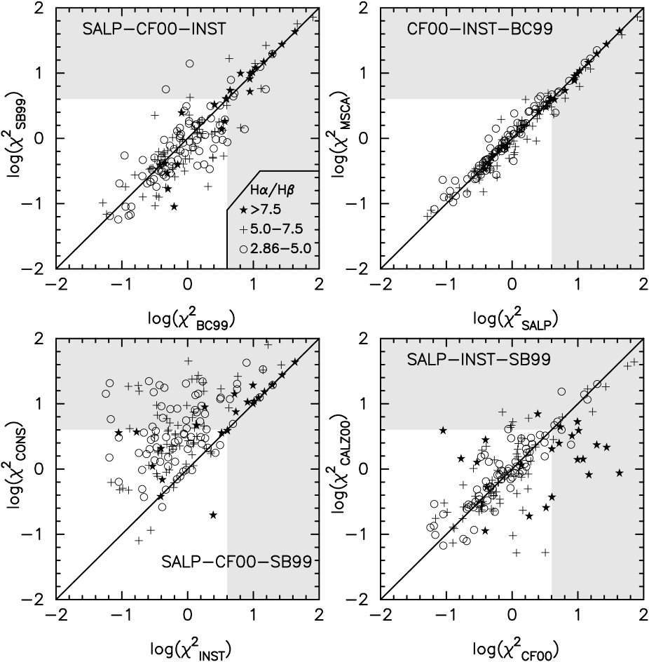
Fig. 4 shows the comparison of $\chi^{2}$ values for several pairs of input models. Information on the $\mathrm{H}\alpha/\mathrm{H}\beta$ emission-line ratios is also shown since extinction turns out to be a crucial parameter in the goodness of the model fits. The shaded area corresponds the zone of poor fits. In the top-left diagram, BC99 and SB99  models with the same of the remaining parameters are compared. Both models provide comparable results for most galaxies.

The bottom-left plot compares instantaneous and continuous star-formation SB99  models. It is quite clear that better fits are obtained for most of the galaxies with short bursts. A large fraction of the continuous star-formation models are rejected by the observations. There are a handful of galaxies with better constant star-formation, but in all cases almost equally good fits are obtained for the burst models.

The top-right diagram shows that the quality of the fits for Miller-Scalo and Salpeter IMFs is indistinguishable. The same is true for the Scalo IMF (not shown). At this point we are not able to establish which of the tested IMFs best reproduces the observed properties of the UCM galaxies. We will return to this issue later.

Finally, the two extinction recipes are compared in the lower-right panel. The CALZ00  recipe seems to yield better fits than the CF00  one for high extinction objects (group of filled stars on the right). On the other hand, for some other galaxies, specially those with low values of the $\mathrm{H}\alpha/\mathrm{H}\beta$ ratio, CF00  works better. For some cases neither provides confident results.

Fig. 5 shows the distribution of the best model fits for the UCM galaxies according to the model input parameters. The $\chi^{2}$ estimator for each galaxy and model has been assumed to be the median of all the 1000 Montecarlo particles and it has been normalized with the number of colours used in its calculation. For each galaxy, we select the model that best-fittings its observational data, i.e showing the lowest value of the $\chi^{2}$ estimator.

A total of 87 objects are best modelled with the SB99  models rather than with the BC99 ones. This corresponds to 53% of the complete sample. On average, these galaxies present redder observed $B-r$ colours and higher $EW(\mathrm{H}\alpha)$ values than the objects best modelled with BC99 models: $(B-r)_{SB99}=0.9\pm 0.3$ vs. $(B-r)_{BC99}=0.7\pm 0.3$ and $EW(H\alpha_{SB99})=60\pm 60$ Å  vs. $EW(H\alpha_{BC99})=110\pm 90$ Å. Moreover, the average metallicity estimated by SB99  models is lower than what BC99 predict. We will discuss these points in Paper II.

We have only used SB99  models with a Salpeter IMF. If we only consider the galaxies best fitted with that IMF, the percentage of best-fittings achieved with this evolutionary code increases to 73%.

Fig. 5 also shows that 82% of the UCM sample is best described by an instantaneous burst of star formation. The objects favouring a constant SFR are characterized by lower extinctions and higher equivalent widths ($\langle E(B-V)\rangle=0.6$ mag and $\langle EW(\mathrm{H}\alpha)\rangle=168$ Å) than those best modelled with instantaneous bursts (0.8 mag and 64 Å).

Among the galaxies best modelled with the BC99 models, two of the IMFs considered seem to dominate over the other one: the most common in this distribution are the Salpeter IMF (42%) and Miller-Scalo’s (42% of the total number of galaxies best fitted by BC99 models). If we also take into account the galaxies modelled with SB99  templates, for 73% of the galaxies a Salpeter IMF yields the best-fittings. These results are in agreement with several studies claiming that a Salpeter slope best reproduces the distribution of stellar masses in massive star formation scenarios (with perhaps a flattening at low masses; see, for example, Massey & Hunter, 1998; Selman et al., 1999; Sakhibov & Smirnov, 2000; Schaerer et al., 2000). However, it is important to emphasise that we have obtained these figures by a simple comparison of the values of the $\chi^{2}$ estimator. A proper discussion on the IMF in UCM galaxies must involve parameters such as the upper mass limit or the fraction of ionizing photons escaping from the birth cloud. This is far beyond the scope of the present paper.

Finally, the CF00  extinction recipe best reproduces the observed colours and gas emission for 55% of the sample. We notice again that high extinctions prevail on the objects best fitted with the CALZ00  law, with $\langle E(B-V)\rangle=0.9\pm 0.5$ (cf. $\langle E(B-V)\rangle=0.6\pm 0.4$ for CF00).

Figure 6: Differences between fitted and measured values for optical and nIR colours, and $EW(\mathrm{H}\alpha)$. Average errors are shown in each panel. Different symbols stand for disk-like, HII-like and AGN galaxies. The data refers to instantaneous SB99  models with a Salpeter IMF and CF00  extinction.

Figure 7: Same as in Fig. 6 but the symbols represent different values of the $\mathrm{H}\alpha/\mathrm{H}\beta$ ratio, an extinction indicator.

Figs. 6 and 7 present residual colour-colour diagrams showing the differences between fitted and measured values for several pairs of observables. Input parameters are SB99  models, instantaneous SFR, Salpeter IMF and CF00  extinction recipe. Information about spectroscopic type (Fig. 6) and $\mathrm{H}\alpha/\mathrm{H}\beta$ ratio (Fig. 7) is also shown in order to search for correlations between these quantities and the goodness of the fit. The median error for each measured colour is indicated by the error bars. In the case of $EW(\mathrm{H}\alpha)$ we have plotted the lines of equality for fitted and measured values.

First, it is clear that the AGNs are not well-fitted (three other AGNs are outside the boundaries of these plots, together with two of the galaxies mentioned at the beginning of this section). As expected, the contribution of the active nucleus cannot be reproduced by the stellar synthesis models. These AGN will be excluded from the rest of the discussion.

A group of objects, mainly disk-like galaxies, exhibit a deficit of observed $B$-band light: their $B-r$ and $B-J$ colours are redder than the best-fit model predictions (e.g., objects with large $\Delta(B-r)$ values in top-left panel). Most of these objects have high $\mathrm{H}\alpha/\mathrm{H}\beta$ ratios. In some cases $\mathrm{H}\beta$ was not detectable. For the galaxies with undetected $\mathrm{H}\beta$, an average $E(B-V)$ based on the spectroscopic type was used initially, but this clearly underestimated the extinction and showed fitted colours which were much bluer than the measured ones. For that reason, we decided to use instead the average of the 25% highest $\mathrm{H}\alpha/\mathrm{H}\beta$ ratios for this spectral class. This value was the one finally assumed and the one used to generate Fig.s 6 and 7. Although this yielded better fits, it seems that we are still somewhat short of the real extinction value for some objects.

At this point it is important to remind the reader that we are using $EW(\mathrm{H}\alpha)$ and $\mathrm{H}\alpha/\mathrm{H}\beta$ values measured in the long-slit spectra, and assume that they are representative of the whole galaxy.

Another group of galaxies have optical-nIR colours which are not well-fitted by the models, such as the object with positive differences in the top-right panel. A visual inspection of these objects reveals that a number of them are high-inclination galaxies (ellipticity larger than 0.3), some with clear dust-lanes best observed in the $B$ images. Examples include UCM0044$+$2246, UCM2255$+$1654 and UCM2329$+$2427. The CF00  extinction recipe fails to model these highly-reddened galaxies (see Fig. 7), while CALZ00  provides better results. Among the 15 worst fitted objects of this kind, 50% have $EW(\mathrm{H}\alpha)$ lower than 30 Å  and virtually all of the rest below 60 Å. The observed $J-K$ colours for these galaxies are also redder than the model predictions, indicating, perhaps, that the underlying old population is more dominant in them.

The problem with extinction gets obviously worse as we move to shorter wavelengths. Some objects may be so extincted that we may be observing just the ‘surface’ of the galaxy disks in $B$ while we can see deeper layers in the nIR (see, for example, Corradi et al., 1996). Since we are observing fewer stars in the blue bands, the measured colours would be redder than what the models predict. Moreover, significant uncertainties still remain in the extinction recipes when trying to match observations spanning a large wavelength range such as optical-nIR colours.

In the diagrams involving the $EW(\mathrm{H}\alpha)$ we see that the models succeed reasonably well in fitting the observed data, although there seems to be a relatively small tendency to underestimate the observed values. Since the measured $\rm H\alpha$ $EW$s are based on long-slit spectroscopy, and thus dominated by the central values, we could be overestimating them if the star formation is significantly more concentrated than the old stars.

4.2 Solution degeneracy

The technique that we have developed to derive the stellar properties of the UCM galaxies is based on the use of the observational errors and a Principal Component Analysis (PCA) study of the solutions. This procedure allows us to obtain information about the degeneracy of the results in the $\{t,b,Z\}$ parameter space. In GdP00  we applied a single linkage hierarchical clustering method (Murtagh & Heck, 1987) in order to study the clustering of solutions achieved in the 1000 Montecarlo particles fitted for each galaxy. That paper pointed out that the clustering pattern is dominated by the discretization in metallicity of the evolutionary synthesis models. Thus, little can be learnt using this clustering method before performing the PCA. Instead, in the present work we have applied the PCA to all the Montecarlo particles and obtained average values and standard deviations for the entire set of solutions of each galaxy.

This method shows that, on average for the complete UCM sample, $69\pm 2$% of the scatter of the Montecarlo particles is represented by the first principal component in the PCA. In less than 3% of the sample this fraction is less than half of the total scatter. In GdP00  the clustering characterization removed the scattering of the solutions due to metallicity. The effect was that the component of the PCA vector in the $Z$ direction was null in most cases. Now the distribution of this component for the whole sample is somewhat flatter, with the strongest peak at $-0.5$ (see Fig. 8). This figure also shows that the age and burst strength components are similar. This means that both quantities are correlated: if we increase the model age, we need to increase the burst strength in order to keep the same $\mathrm{H}\alpha$ equivalent width. Moreover, since the strongest peak in the metallicity direction has opposite sign to the other two, there is an age-metallicity degeneracy (anti-correlation).

Figure 8: Histograms of the 3 components of the first vector of the PCA for the UCM Survey galaxies. The plot refers to SB99  models, Salpeter IMF, instantaneous burst and CALZ00  recipe.

5 Summary

In this paper, the first of a series, we have described a method to derive the properties of the star-formation and the stellar populations in star-forming galaxies using broad-band photometry and spectroscopy. We also present the available data for the UCM Survey galaxies, covering the optical and nIR spectral ranges. The technique is based on the assumption that our galaxies have a composite stellar population. The evolved component resembles that of a typical quiescent spiral/lenticular galaxy, whereas the young stellar population component is generated with an evolutionary synthesis model. This fact means that our modelling refers to the properties of a recent star formation event which takes place in excess of what is typical in a normal spiral or lenticular galaxy. The model parameters considered are: (1) stellar evolutionary synthesis (the Bruzual & Charlot 1999 and Leitherer et al. 1999 models); (2) IMFs (Salpeter, 1955; Scalo, 1986; Miller & Scalo, 1979); (3) star formation modes (instantaneous and constant); and (4) extinction recipes (Calzetti et al. 2000 and Charlot & Fall 2000).

We have developed a statistical tool that takes into account the observational uncertainties and a careful interpretation of the model fits. The procedure is tested with the UCM sample data, and used to study the dependence of the goodness of the model fits on several a priori input parameters. We find that our modelling is able to reproduce the photometric and spectroscopic properties of almost all the star-forming galaxies of the UCM Survey. Our test on the a priori model parameter choices, based on our $\chi^{2}$ estimator, reveals that:

• both SB99  and BC99 models provide reasonable and comparable fits. The SB99  models provide marginally better results, in particular for redder galaxies with relatively higher $\mathrm{H}\alpha$ equivalent widths.

• UCM galaxies clearly show a preference for instantaneous bursts of recent star formation rather than constant star-formation rates.

• The models with a Salpeter initial mass function better reproduce the observations for nearly 75% of the sample, although a number of galaxies also present best results using the other IMFs and this result must be regarded with caution.

• The extinction description developed by CF00  yields satisfactory results for the majority of our sample galaxies (with a variation in the extinction law), but it fails to reproduce the properties of high extinction objects.

Among all the possible combinations of input parameters, an important number of galaxies (one third) is best modelled with SB99  code, Salpeter IMF, instantaneous SFR and CF00  extinction recipe.

In Paper II, we will use the techniques developed here to study, in detail, the properties of the UCM galaxies.

References

- Abraham & van den Bergh (2002) Abraham R. G., van den Bergh S., 2002, in Disks of Galaxies: Kinematics, Dynamics and Perturbations. ASP Conference Proceedings, Vol. 275. Edited by E. Athanassoula. A. Bosma and R. Mujica. ISBN: 1-58381-117-6. Puebla, Mexico., eds. Athanassoula E., Bosma A., Mujica R., Disks of Galaxies: Kinematics, Dynamics and Perturbations
- Alonso et al. (1999) Alonso O., García-Dabó C. E., Zamorano J., Gallego J., Rego M., 1999, ApJS, 122, 415
- Aragón-Salamanca et al. (1993) Aragón-Salamanca A., Ellis R. S., Couch W. J., Carter D., 1993, MNRAS, 262, 764
- Balzano (1983) Balzano V. A., 1983, ApJ, 268, 602
- Bell & de Jong (2000) Bell E. F., de Jong R. S., 2000, MNRAS, 312, 497
- Bell & de Jong (2001) Bell E. F., de Jong R. S., 2001, ApJ, 550, 212
- Brocklehurst (1971) Brocklehurst M., 1971, MNRAS, 153, 471
- Cairós et al. (2001) Cairós L. M., Vílchez J. ., González Pérez J. . ., Iglesias-Páramo J., Caon N., 2001, ApJS, 133, 321
- Calzetti (2001) Calzetti D., 2001, PASP, 113, 1449
- Calzetti et al. (2000) Calzetti D., Armus L., Bohlin R. C., Kinney A. L., Koornneef J., Storchi-Bergmann T., 2000, ApJ, 533, 682
- Cardelli et al. (1989) Cardelli J. A., Clayton G. C., Mathis J. S., 1989, ApJ, 345, 245
- Charlot & Fall (2000) Charlot S. ., Fall S. M., 2000, ApJ, 539, 718
- Charlot & Longhetti (2001) Charlot S. ., Longhetti M., 2001, MNRAS, 323, 887
- Corradi et al. (1996) Corradi R. L. M., Beckman J. E., Simonneau E., 1996, MNRAS, 282, 1005
- Davidge (1992) Davidge T. J., 1992, AJ, 103, 1512
- Doublier et al. (2001) Doublier V., Caulet A., Comte G., 2001, A&A, 367, 33
- Elias et al. (1982) Elias J. H., Frogel J. A., Matthews K., Neugebauer G., 1982, AJ, 87, 1029
- Ellis (1997) Ellis R. S., 1997, ARA&A, 35, 389
- Ferguson et al. (2000) Ferguson H. C., Dickinson M., Williams R., 2000, ARA&A, 38, 667
- Ferland (1980) Ferland G. J., 1980, PASP, 92, 596
- Fioc & Rocca-Volmerange (1999) Fioc M., Rocca-Volmerange B., 1999, A&A, 351, 869
- Fukugita et al. (1995) Fukugita M., Shimasaku K., Ichikawa T., 1995, PASP, 107, 945
- Gallego (1998) Gallego J., 1998, Ap&SS, 263, 1
- Gallego et al. (1995) Gallego J., Zamorano J., Aragón-Salamanca A., Rego M., 1995, ApJL, 455, L1
- Gallego et al. (1996) Gallego J., Zamorano J., Rego M., Alonso O., Vitores A. G., 1996, A&AS, 120, 323
- Gil de Paz et al. (2000a) Gil de Paz A., Aragón-Salamanca A., Gallego J., Alonso-Herrero A., Zamorano J., Kauffmann G., 2000a, MNRAS, 316, 357
- Gil de Paz & Madore (2002) Gil de Paz A., Madore B. F., 2002, AJ, 123, 1864
- Gil de Paz et al. (2000b) Gil de Paz A., Zamorano J., Gallego J., 2000b, A&A, 361, 465
- Gil de Paz et al. (2000c) Gil de Paz A., Zamorano J., Gallego J., Domínguez F. D., 2000c, A&AS, 145, 377
- González Delgado et al. (1999) González Delgado R. M., Leitherer C., Heckman T. M., 1999, ApJS, 125, 489
- Guzmán et al. (1997) Guzmán R., Gallego J., Koo D. C., Phillips A. C., Lowenthal J. D., Faber S. M., Illingworth G. D., Vogt N. P., 1997, ApJ, 489, 559
- Hawarden et al. (2001) Hawarden T. G., Leggett S. K., Letawsky M. B., Ballantyne D. R., Casali M. M., 2001, MNRAS, 325, 563
- Hughes et al. (1998) Hughes D. H., Serjeant S., Dunlop J., Rowan-Robinson M., Blain A., Mann R. G., Ivison R., Peacock J., Efstathiou A., Gear W., Oliver S., Lawrence A., Longair M., Goldschmidt P., Jenness T., 1998, Nature, 394, 241
- Hunt et al. (1998) Hunt L. K., Mannucci F., Testi L., Migliorini S., Stanga R. M., Baffa C., Lisi F., Vanzi L., 1998, AJ, 115, 2594
- Iwamuro et al. (2000) Iwamuro F., Motohara K., Maihara T., Iwai J., Tanabe H., Taguchi T., Hata R., Terada H., Oya M. G. S., Iye M., Yoshida M., Karoji H., Ogasawara R., Sekiguchi K., 2000, PASJ, 52, 73
- Jarrett et al. (2000) Jarrett T. H., Chester T., Cutri R., Schneider S., Skrutskie M., Huchra J. P., 2000, AJ, 119, 2498
- Kennicutt (1983) Kennicutt R. C., 1983, ApJ, 272, 54
- Krüger et al. (1995) Krüger H., Fritze-v. Alvensleben U., Loose H.-H., 1995, A&A, 303, 41
- Kurucz (1992) Kurucz R. L., 1992, in IAU Symp. 149: The Stellar Populations of Galaxies. Kluwer Academic Publishers, Dordrecht. Angra dos Reis (Brazil), 1991 August., eds. Barbuy B., Renzini A., Vol. 149, Model Atmospheres for Population Synthesis. p. 225
- Leitherer et al. (1999) Leitherer C., Schaerer D., Goldader J. D., Delgado R. M. G. ., Robert C., Kune D. F., de Mello D. . F., Devost D., Heckman T. M., 1999, ApJS, 123, 3
- Loose & Thuan (1985) Loose H. H., Thuan T. X., 1985, in Star Forming Dwarf Galaxies and Related Objects. Editions Frontières, Gif sur Yvette, eds. Kunth D., Thuan T. X., Tran T. V., The Morphology and Structure of Blue Compact Dwarf Galaxies from CCD Observations. p. 73
- Massey & Hunter (1998) Massey P., Hunter D. A., 1998, ApJ, 493, 180
- Miller & Scalo (1979) Miller G. E., Scalo J. M., 1979, ApJS, 41, 513
- Moorwood et al. (2000) Moorwood A. F. M., van der Werf P. P., Cuby J. G., Oliva E., 2000, A&A, 362, 9
- Murtagh & Heck (1987) Murtagh F., Heck A., 1987, Multivariate data analysis (Astrophysics and Space Science Library, Dordrecht: Reidel, 1987)
- Osterbrock (1989) Osterbrock D. E., 1989, Astrophysics of gaseous nebulae and active galactic nuclei (Research supported by the University of California, John Simon Guggenheim Memorial Foundation, University of Minnesota, et al. Mill Valley, CA, University Science Books, 1989, 422 p.)
- Papaderos et al. (1996) Papaderos P., Loose H.-H., Thuan T. X., Fricke K. J., 1996, A&AS, 120, 207
- Pascual et al. (2001) Pascual S., Gallego J., Aragón-Salamanca A., Zamorano J., 2001, A&A, 379, 798
- Pérez-González et al. (2001) Pérez-González P. G., Gallego J., Zamorano J., Gil de Paz A., 2001, A&A, 365, 370
- Pérez-González et al. (2002a) Pérez-González P. G., Gil de Paz A., Zamorano J., Gallego J., 2002a, ApJ, in preparation
- Pérez-González et al. (2002b) Pérez-González P. G., Gil de Paz A., Zamorano J., Gallego J., Alonso-Herrero A., Aragón-Salamanca A., 2002b, MNRAS, in press, astro-ph/0209397
- Pérez-González et al. (2002c) Pérez-González P. G., Zamorano J., Gallego J., Aragón-Salamanca A., Gil de Paz A., 2002c, ApJ, in preparation
- Pérez-González et al. (2000) Pérez-González P. G., Zamorano J., Gallego J., Gil de Paz A., 2000, A&AS, 141, 409
- Persson et al. (1998) Persson S. E., Murphy D. C., Krzeminski W., Roth M., Rieke M. J., 1998, AJ, 116, 2475
- Pettini et al. (1998) Pettini M., Kellogg M., Steidel C. C., Dickinson M., Adelberger K. L., Giavalisco M., 1998, ApJ, 508, 539
- Pettini et al. (2001) Pettini M., Shapley A. E., Steidel C. C., Cuby J., Dickinson M., Moorwood A. F. M., Adelberger K. L., Giavalisco M., 2001, ApJ, 554, 981
- Sakhibov & Smirnov (2000) Sakhibov F., Smirnov M., 2000, A&A, 354, 802
- Salpeter (1955) Salpeter E. E., 1955, ApJ, 121, 161
- Salzer et al. (1989) Salzer J. J., MacAlpine G. M., Boroson T. A., 1989, ApJS, 70, 479
- Scalo (1986) Scalo J. M., 1986, Fundamentals of Cosmic Physics, 11, 1
- Schaerer et al. (2000) Schaerer D., Guseva N. G., Izotov Y. I., Thuan T. X., 2000, A&A, 362, 53
- Schlegel et al. (1998) Schlegel D. J., Finkbeiner D. P., Davis M., 1998, ApJ, 500, 525
- Schmidt & Green (1983) Schmidt M., Green R. F., 1983, ApJ, 269, 352
- Selman et al. (1999) Selman F., Melnick J., Bosch G., Terlevich R., 1999, A&A, 347, 532
- Steidel et al. (1999) Steidel C. C., Adelberger K. L., Giavalisco M., Dickinson M., Pettini M., 1999, ApJ, 519, 1
- Steidel et al. (1996) Steidel C. C., Giavalisco M., Pettini M., Dickinson M., Adelberger K. L., 1996, ApJL, 462, L17
- Trager et al. (1998) Trager S. C., Worthey G., Faber S. M., Burstein D., González J. J., 1998, ApJS, 116, 1
- Tresse et al. (2001) Tresse L., Maddox S., Le Fevre O., Cuby J., 2001, MNRAS, astro-ph/0111390
- van der Werf et al. (2000) van der Werf P. P., Moorwood A. F. M., Bremer M. N., 2000, A&A, 362, 509
- Vitores et al. (1996a) Vitores A. G., Zamorano J., Rego M., Alonso O., Gallego J., 1996a, A&AS, 118, 7
- Vitores et al. (1996b) Vitores A. G., Zamorano J., Rego M., Gallego J., Alonso O., 1996b, A&AS, 120, 385
- Wainscoat & Cowie (1992) Wainscoat R. J., Cowie L. L., 1992, AJ, 103, 332
- Yan et al. (2000) Yan L., McCarthy P. J., Weymann R. J., Malkan M. A., Teplitz H. I., Storrie-Lombardi L. J., Smith M., Dressler A., 2000, AJ, 120, 575
- Zamorano et al. (1996) Zamorano J., Gallego J., Rego M., Vitores A. G., Alonso O., 1996, ApJS, 105, 343
- Zamorano et al. (1994) Zamorano J., Rego M., Gallego J. G., Vitores A. G., González-Riestra R., Rodríguez-Caderot G., 1994, ApJS, 95, 387