Nonlinear clustering during the cosmic Dark Ages and its effect on the 21-cm background from minihalos

Abstract

Hydrogen atoms inside virialized minihalos (with $T_{\rm vir}\leq 10^{4}{\rm K}$) generate a radiation background from redshifted 21-cm line emission whose angular fluctuations reflect clustering during before and during reionization. We have shown elsewhere that this emission may be detectable with the planned Low Frequency Array (LOFAR) and Square Kilometer Array (SKA) in a flat Cold Dark Matter Universe with a cosmological constant ($\Lambda$CDM). This is a direct probe of structure during the “Dark Ages” at redshifts $z\ga 6$ and down to smaller scales than have previously been constrained. In our original calculation, we used a standard approximation known as the “linear bias” [e.g. Mo & White (1996)]. Here we improve upon that treatment by considering the effect of nonlinear clustering. To accomplish this, we develop a new analytical method for calculating the nonlinear Eulerian bias of halos, which should be useful for other applications as well. Predictions of this method are compared with the results of $\Lambda$CDM N-body simulations, showing significantly better agreement than the standard linear bias approximation. When applied to the 21-cm background from minihalos, our formalism predicts fluctuations that differ from our original predictions by up to 30% at low frequencies (high-$z$) and small scales. However, within the range of frequencies and angular scales at which the signal could be observable by LOFAR and SKA as currently planned, the differences are small and our original predictions prove robust. Our results indicate that while a smaller frequency bandwidth of observation leads to a higher signal that is more sensitive to nonlinear effects, this effect is counteracted by the lowered sensitivity of the radio arrays. We calculate the best frequency bandwidth for these observations to be $\Delta\nu_{\rm obs}\sim 2$ MHz. Finally we combine our simulations with our previous calculations of the 21-cm emission from individual minihalos to construct illustrative radio maps at $z=9$.

1 Introduction

Despite striking progress over the past decade, cosmologists have still failed to see into the “Dark Ages” of cosmic time. Although the details of this epoch between recombination at redshift $z\sim 10^{3}$ and reionization at $z\ga 6$ are crucial for understanding issues ranging from early structure formation to the process of reionization itself, no direct observations of any kind have been made in this redshift range. Recently, we made the first proposal for such direct observations (Iliev et al. 2002, from hereafter Paper I) based on collisional excitation of the hydrogen 21-cm line in the warm, dense, neutral gas in virialized minihalos (halos with virial temperature $T_{\rm vir}\leq 10^{4}{\rm K}$), the first baryonic structures to emerge in the standard CDM universe. We showed that collisional excitation is sufficient to increase the spin temperature of hydrogen atoms inside minihalos above the temperature the cosmic microwave background (CMB). Minihalos should generally appear in emission with respect to the CMB, producing a background “21-cm forest” of redshifted emission lines, well-separated in frequency. Unlike all previous works (Hogan & Rees, 1979; Scott & Rees, 1990; Subramanian & Padmanabhan, 1993; Madau, Meiksen & Rees, 1997; Shaver et al., 1999; Tozzi et al., 2000), this mechanism does not require sources of Ly$\alpha$ radiation for “pumping” the 21-cm line and decoupling it from the CMB.

In Paper I we calculated the 21-cm emission properties of individual minihalos in detail, along with the total background and its large-scale fluctuations due to clustering. Although individual lines and the overall background are too weak to be readily detected, the background fluctuations should be measurable on $\sim 10^{\prime}-100^{\prime}$ scales with the currently-planned radio arrays LOFAR and SKA. We demonstrated that such observations can be used to probe the details of reionization as well as measure the power spectrum of density fluctuations at far smaller scales than have been constrained previously.

In the current paper we extend these results to smaller scales. Our previous calculations showed that the fluctuation signal increases as the beam size and frequency bandwidth decrease, which corresponds to sampling the 21-cm emission from minihalos within smaller volumes. As these volumes correspond in turn to length scales that are more nonlinear, nonlinear effects have the greatest impact on the angular scales and frequency bandwidths at which the signal is the strongest.

This issue is of particular importance as our previous investigations relied on the standard, simplified nonlinear bias of Mo & White (1996), which breaks down at many of the relevant redshifts and length scales. For example, an rms density fluctuation in a Cold Dark Matter universe with a cosmological constant ($\Lambda$CDM) at $z=6(8),$ is strongly nonlinear ($\sigma(M)\geq 1$) for $M\leq 10^{9}M_{\odot}$ ($6.2\times 10^{7}M_{\odot}$), which roughly corresponds to the region sampled by beam sizes 9” (3”), for frequency bandwidths 12 kHz (3 kHz), respectively. Nonlinear effects can influence the predicted background fluctuations on even larger scales, up to few comoving Mpc (corresponding to few hundred kHz frequency bandwidths and 1-10 arc min beams), even if these scales are still not strongly nonlinear. Additionally, rare halos are always more strongly clustered than the underlying density distribution (i.e. the bias is $>1$), again bringing nonlinear issues to the fore.

In order to address these important issues we have carried out a series of high-redshift N-body simulations of small scale structure formation, which we use to construct 21-cm line radio maps that illustrate the expected fluctuations in the emission. As no current simulations are able to span the full dynamic range relevant to 21-cm emission, however, we extend our results by developing a new formalism for calculating the nonlinear Eulerian bias of halos, which is based on the Lagrangian bias formalism of Scannapieco & Barkana (2002, hereafter SB02). We describe this approach in detail in this paper, verify it by comparing it with the results of our N-body simulations, and apply it to to calculate improved predictions for the fluctuations in the 21-cm emission. These are then compared to the predictions given in Paper I, quantifying the impact of nonlinear effects on minihalo emission.

The structure of this work is as follows. In § 2 we describe a set of simulations of minihalo emission at high redshift, and use these to construct simulated maps at small angular scales. In § 3 we present our improved calculation of the Eulerian bias and verify it by comparison with the numerical simulations presented in § 2. In § 4 we modify the calculation of the radiation background from minihalos to incorporate the contribution due to nonlinear clustering of sources, according to the formalism described in § 3, and describe the results of our nonlinear formalism. Conclusions are given in § 5.

2 Numerical simulations and simulated 21-cm radio maps

We simulated the formation of minihalos in three cubic computational volumes of comoving size 1 Mpc, 0.5 Mpc, and 0.25 Mpc, respectively. We used a standard Particle-Particle/Particle-Mesh (P³M) algorithm (Hockney & Eastwood 1981), with $128^{3}$ equal-mass particles, a $256^{3}$ PM grid, and a softening length of 0.3 grid spacing. Here and throughout this paper we consider a flat $\Lambda$CDM model with density parameter $\Omega_{0}=0.3$, cosmological constant $\lambda_{0}=0.7$, Hubble constant $H_{0}=70\,\rm km\,s^{-1}Mpc^{-1}$, baryon density parameter $\Omega_{b}=0.02h^{-2}$ (where $h=H_{0}/100\,\rm km\,s^{-1}Mpc^{-1}$), and no tilt. The initial conditions where generated using the transfer function of Bardeen et al. (1986) with the normalization of Bunn & White (1997) (for details, see Martel & Matzner 2000, §2). All simulations started at redshift $z=50$ and terminated at redshift $z=9$. To identify minihalos, we used a standard friends-of-friends algorithm with a linking length equal to 0.25 times the mean particle spacing. We rejected halos composed of 20 particles or less. Table 1 lists the comoving size $L_{\rm box}$ of the box, the comoving value of the softening length $\eta$, the total mass $M_{\rm tot}$ inside the box, and the particle mass $M_{\rm part}$.

Once the halos are identified, we can use their properties and distribution to compute the corresponding radio maps. We assign to each halo a 21-cm flux based on its mass and redshift of formation by modeling the halos as Truncated Isothermal Spheres (Shapiro, Iliev & Raga, 1999; Iliev & Shapiro, 2001). The 21-cm fluxes from individual minihalos are obtained by solving the radiative transfer equation self-consistently through each halo to obtain the line-integrated flux, as described in Paper I. Let us consider a cylindrical volume with radius $R=\Delta\theta_{\rm beam}(1+z)D_{A}(z)/2$, and length $L_{\rm box}$ , where $D_{A}(z)$ is the angular diameter distance, $\Delta\theta_{\rm beam}$ is the beam size of the observation. Then the beam-averaged differential antenna temperature $\overline{\delta T}_{b}$ is calculated using equation 6 of Paper I, which can be discretized as follows:

$$\overline{\delta T}_{b}({\bf x})={c(1+z)^{4}\over 2\nu_{0}H(z)}{1\over\pi R^{2}L_{\rm box}}\sum_{i}(\Delta\nu_{\rm eff})_{i}(\delta T_{b,\nu_{0}})_{i}A_{i}e^{-({\bf x}-{\bf x}_{i})^{2}/2R^{2}}\,,$$ (1)

where $H(z)$ is the Hubble constant at redshift $z$, $\nu_{0}$ is the rest-frame line frequency, $\pi R^{2}L_{\rm box}$ is the comoving volume of the beam $(\Delta\nu_{\rm eff})_{i}$, $(\delta T_{b,\nu_{0}})_{i}$, and $A_{i}$ are the effective line width, the line-center differential brightness temperature, and the geometric cross-section of halo $i$, respectively, and we use Gaussian filter in order to ensure that the contribution of a particular minihalo to a particular pixel varies smoothly with the location of the minihalo.

Table 1: Parameters of the N-body simulations

$L_{\rm box}$ (Mpc)	$\eta$ (kpc)	$M_{\rm tot}(M_{\odot})$	$M_{\rm part}(M_{\odot})$
1.0	1.172	$4.079\times 10^{10}$	$1.945\times 10^{4}$
0.5	0.586	$5.099\times 10^{9}$	$2.431\times 10^{3}$
0.25	0.293	$6.374\times 10^{8}$	$3.039\times 10^{2}$

The resulting maps are shown in Figure 1. Due to the small box sizes that are required to resolve the minihalos, the beams used to produce the maps are also very small, ranging from 4” to 0.25”. The fluxes from such small beam sizes are well below the sensitivity limits of the currently planned radio arrays LOFAR and SKA. Additionally, the larger-box (1 Mpc and 0.5 Mpc) simulations do not have sufficient mass resolution to resolve the smallest halos, while the larger-mass minihalos are not present in the smaller box simulations. Therefore the flux levels are somewhat underestimated in all cases, and should be considered only as illustrative of fluctuations on very small scales.

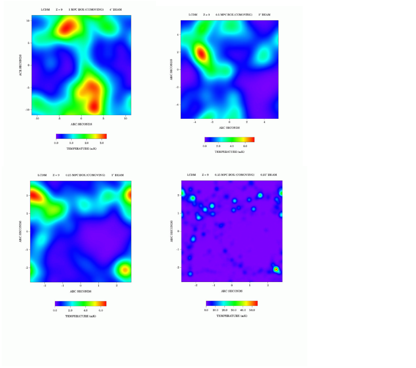
Figure 1: (upper panels) Differential brightness temperature radio map of the 21-cm emission from minihalos at $z=9$, produced as described in the text from $\Lambda$CDM N-body simulation of: (upper left panel) box size 1 Mpc and beam size $\Delta\theta_{\rm beam}=4^{\prime\prime}$, and (upper right panel) box size 0.5 Mpc and beam size $\Delta\theta_{\rm beam}=2^{\prime\prime}.$ (lower left panel) box size 0.25 Mpc and $\Delta\theta_{\rm beam}=1^{\prime\prime}$, and (lower right panel) box size 0.25 Mpc and $\Delta\theta_{\rm beam}=0.25^{\prime\prime}$.

3 Nonlinear clustering regime and comparison to simulations

3.1 An analytic approach to nonlinear clustering

As our simulations are unable to span a sufficient range of scales to both resolve all minihalos and reproduce the physical scales accessible to observations, we adopt instead an alternate technique to estimate the full nonlinear signal. We apply an approximate formalism that is an extension of the one developed in SB02. A more complete discussion of this method, refinement of the basic formalism, and detailed comparisons with simulations will be presented in a separate paper. In this section we summarize the basic features of this approach and show that it is sufficient for our purposes in this investigation. For an alternative approach see Catelan, Matarese, & Porciani (1998).

In SB02 the authors extended the Press-Schechter formalism as reinterpreted by Bond et al. (1991) to calculate the number density of collapsed objects in two regions of space initially separated by a fixed comoving distance. In this approach virialized halos are associated with linear density peaks that fall above a critical value usually taken to be $\delta_{c}=1.686.$ Here the linear overdensity field is defined as $\delta({\bf x})D^{-1}(z)\equiv\rho({\bf x},z)/\bar{\rho}(z)-1$, where $\rho({\bf x})$ is the linear mass density as a function of position and and $\bar{\rho}$ is the mean mass density. Note that here the linear overdensity field $\delta({\bf x})$ is described in terms of its value extrapolated to $z=0$, and its evolution with time is subsumed by the “linear growth factor” $D(z)=\delta(0)/\delta{(z)}.$ Other choices for $\delta_{c}$ and its evolution have been explored in the literature, by fitting to simulations (Sheth, Mo, & Tormen, 2001; Jenkins et al., 2001) or incorporating the Zel’dovich or adhesion approximations (Lee & Shandarin, 1999; Menci, 2001). While these methods improve the accuracy of the Press-Schechter technique, they provide no information about nonlinear clustering. Here we strive to develop a formalism that is applicable to nonlinear clustering regardless of the recipe chosen for $\delta_{c}$.

Once $\delta_{c}$ determined, the presence of a halo can be associated with a random walk procedure. At a given redshift we consider the smoothed density in a region around a point in space. We begin by averaging over a large mass scale $M$, or equivalently, by including only small comoving wavenumbers $k$. We then lower $M,$ adding $k$ modes, and adjusting $\delta(M)$ accordingly. This amounts to a random walk in which the “time variable” is the variance associated with the filter mass and the “spatial variable” is the overdensity itself. This walk continues until the averaged overdensity crosses $\delta_{c}D^{-1}(z)$ and we assume that the point belongs to a halo with a mass $M$ corresponding to this filter scale.

The problem of halo collapse at two positions in space can be similarly associated with two random walks in the presence of a barrier of height $\delta_{c}D^{-1}(z)$. These random walks are extremely correlated at large scales, and become less and less so as the modes of smaller and smaller scales are added. In SB02 this process was approximated by a completely correlated random walk down to an overall variance $S$ = $\xi$, where $\xi$ is the correlation function that accounts for the excess probability of finding a second halo at a fixed distance from a given halo. This correlated random walk was then followed by uncorrelated walks down to the final variances associated with the masses of the objects, $S=\sigma^{2}(M_{1})$ and $\sigma^{2}(M_{2}).$

This procedure lends itself directly to calculating the overall increase in number density due to infall. The fact that the overdensity on large scales will contract the distances between halos provides an additional contribution at the length scale $x$ such that $\sigma^{2}(x)=\xi$, the scale down to which the evolution of the two points is completely correlated. Let $\delta_{0}$ be the linear overdensity at redshift zero at that scale. The probability distribution of $\delta_{0}$, $Q_{0}$ is then simply given by a Gaussian, with a barrier imposed at $\nu(z)\equiv\delta_{c}D^{-1}(z)$:

$$Q_{0}(\nu,\delta_{0},\xi)=[G(\delta_{0},\xi)-G(2\nu-\delta_{0},\xi)]\,\theta(\nu-\delta_{0}),$$ (2)

where $G(\delta,\xi)\equiv(2\pi\xi)^{-1/2}e^{-\delta^{2}/2\xi}$, and $\theta$ is the Heaviside step function.

We now consider $f_{2}(\nu(z),\sigma^{2}_{1},\sigma^{2}_{2},\delta_{0},\xi)\,d\sigma^{2}_{1}\,d\sigma^{2}_{2}$, the joint probability of having point $A$ in a halo with mass corresponding to the range $\sigma^{2}_{1}$ to $\sigma^{2}_{1}+d\sigma^{2}_{1}$ and point $B$ in a halo with mass corresponding to the range $\sigma^{2}_{2}$ to $\sigma^{2}_{2}+d\sigma^{2}_{2}$, whose random walks pass though a value of $\delta_{0}$ at the $\sigma^{2}(M)=\xi$ scale. In this case we obtain an expression analogous to equation (37) of SB02

$$f_{2}(\nu(z),\delta_{0},\sigma^{2}_{1},\sigma^{2}_{2},\xi(r)) = \frac{\partial}{\partial\sigma^{2}_{1}}\frac{\partial}{\partial\sigma^{2}_{2}}\left[2\int_{-\infty}^{\nu(z)}d\delta_{1}-\int_{-\infty}^{\infty}d\delta_{1}\right]\left[2\int_{-\infty}^{\nu(z)}d\delta_{2}-\int_{-\infty}^{\infty}d\delta_{2}\right]Q_{12}(\nu,\delta_{1},\delta_{2},\sigma^{2}_{1},\sigma^{2}_{2},\xi(r)),$$ (3)

where now $Q_{12}\equiv G(\delta_{1}-\delta_{0},\sigma^{2}_{1}-\xi)G(\delta_{2}-\delta_{0},\sigma^{2}_{2}-\xi)$, and the reader is referred to SB02 for a more detailed derivation of $f_{2}$ from the underlying probability distribution.

Averaging equation (3) over the probability distribution for $\delta_{0}$ as given in equation (2) and carrying out the partial derivatives we obtain the Eulerian “bivariate” number density, the joint probability of having point $A$ lie in a halo in the mass range $M_{1}$ to $M_{1}+dM_{1}$ and point $B$ at a comoving distance $r$ lie in a halo in the mass range $M_{2}$ to $M_{2}+dM_{2}$ at a redshift $z$:

$$\frac{d^{2}n^{2}_{12,E}}{dM_{1}dM_{2}}(r,z)=\frac{\bar{\rho}}{M_{1}}\left|\frac{d\sigma^{2}_{1}}{dM_{1}}\right|\frac{\bar{\rho}}{M_{2}}\left|\frac{d\sigma^{2}_{2}}{dM_{2}}\right|\left(1-\frac{\partial\xi}{\partial\sigma^{2}_{1}}\right)\left(1-\frac{\partial\xi}{\partial\sigma^{2}_{2}}\right)f_{2,E}(\nu(z),\sigma^{2}_{1},\sigma^{2}_{2},\xi(r)),$$ (4)

where

$$f_{2,E}(\nu,\sigma^{2}_{1},\sigma^{2}_{2},\xi)\equiv\int_{-\infty}^{\nu}d\delta_{0}Q_{0}(\delta_{0},\xi)\,g(D^{-1}\delta_{0})\,f(\nu-\delta_{0},\xi-\sigma^{2}_{1})\,g(D^{-1}\delta_{0})f(\nu-\delta_{0},\xi-\sigma^{2}_{2}),$$ (5)

and $f(\nu,\sigma^{2})\equiv(2\pi)^{-1/2}(\nu/\sigma^{3})e^{-\nu^{2}/2\sigma^{2}}$. Here $g(D^{-1}\delta_{0})$ is $\rho/\bar{\rho}$ at the scale at which the points $A$ and $B$ are completely correlated. This can be thought of as the contraction of a large spherical perturbation that surrounds both points and contains a total mass $M$ of material, where $\sigma^{2}(M)=\xi$. This contribution is then just $(1+D^{-1}\delta_{0})$ in the linear regime, and for our purposes here we assume $g(D^{-1}\delta_{0})=(1+D^{-1}\delta_{0})$ for all values as this reproduces well the results from simulations.

Finally we define the Eulerian bias as

$$b_{E}^{2}\xi\,D^{-2}\equiv\frac{d^{2}n^{2}_{12,E}}{dM_{1}dM_{2}}\left(\frac{dn_{1,E}}{dM_{1}}\frac{dn_{2,E}}{dM_{2}}\right)^{-1}-1$$ (6)

where we divide by $dn_{E}/dM$, a single point number density that accounts for the self correlations between the collapsed peaks and the overdense sphere, which are over-counted in equation (4). To compute this probability we again carry out an average over the probability distribution (2), but in this case we consider $f_{1}(\nu,\delta_{0},\sigma^{2}_{1})d\sigma^{2}_{1}=f(\nu-\delta_{0},\sigma^{2}-\xi)d\sigma^{2}_{1},$ the probability of having a single point in a halo with a mass corresponding to the range $\sigma^{2}_{1}$ to $\sigma^{2}_{1}+d\sigma^{2}_{1}$ whose random walk passes through $\delta_{0}$ at the $\sigma^{2}(M)=\xi$ scale. This gives $dn_{E}/dM=(\bar{\rho}/M)\,|d\sigma^{2}\!/dM|\,(1+\partial\xi/\partial\sigma^{2})f_{E}(\nu,\sigma^{2})$ where

$$f_{E}(\nu,\sigma^{2},\xi)\equiv\int_{-\infty}^{\nu}d\delta_{0}Q_{0}(\delta_{0},\nu,\xi)g(\delta_{0}D^{-1})f(\nu-\delta_{0},\xi-\sigma^{2}).$$ (7)

Combining these expressions yields our final expression for the bias

$$b_{E}^{2}\xi D^{-2}=\frac{f_{2,E}(\nu,\sigma^{2}_{1},\sigma^{2}_{2},\xi)}{f_{E}(\nu,\sigma^{2}_{1},\xi)\,f_{E}(\nu_{2},\sigma^{2}_{2},\xi)}-1.$$ (8)

Note that at large distances we can work to order $\delta_{0}^{2}$ to determine the asymptotic limit as $\xi/\sigma^{2}\longrightarrow 0.$ In this limit

$$g(\delta_{0}D^{-1})f(\nu-\delta_{0},\sigma^{2}-\xi)\longrightarrow\left[1-D^{-1}\,\delta_{0}\left(\frac{\nu^{2}}{\delta_{c}\sigma^{2}}-\frac{1}{\delta_{c}}+1\right)+{\cal O}(\delta_{0}^{2})\right]f(\nu,\sigma^{2}-\xi),$$ (9)

and the only surviving term in equation (8) is the cross term between terms of order $\delta_{0}$. All other terms cancel out between the numerator and the denominator, giving

$$b_{E}^{2}=\left(1+\frac{\nu/\sigma^{2}_{1}-1}{\delta_{c}}\right)\left(1+\frac{\nu/\sigma^{2}_{2}-1}{\delta_{c}}\right),$$ (10)

Thus our formalism reproduces the usual bias as in Mo & White (1996) at large distance, as was used in Paper I.

Finally, we define the flux-averaged correlation between objects as

$$\bar{b}_{E}^{2}\xi D^{-2}=\frac{\int dM_{1}\,\int dM_{2}\,F(M_{1})({dn}/{dM_{1}})\,F(M_{2})({dn}/{dM_{2}})\,b_{E}^{2}\xi D^{-2}}{\left[\int dM\,F(M)({dn}/{dM})\right]^{2}},$$ (11)

where $F(M)$ is the line-integrated flux of a minihalo of mass $M$.

3.2 Nonlinear properties and comparisons with simulations

Figure 2: Comparison of standard and nonlinear bias. In all panels, the solid curves give $b_{E}^{2}D^{-2}\xi$ as calculated in equation (8) while the dotted lines give the standard bias expressions as used in Paper I. For each case, the upper curves assume a fixed mass of $10^{7}M_{\odot}$, corresponding to a spherical perturbation with a comoving radius of approximately $38$ kpc, while the lower curves assume a fixed mass of $10^{6}M_{\odot}$, corresponding to a comoving radius of $18$ kpc.

In Fig. 2 we plot $b_{E}^{2}\xi D^{-2}$ as calculated from equation (8) and the standard expression, equation (10), using the fit to the density fluctuation power spectrum given by Eisenstein & Hu (1999). In each panel we show the behavior of $10^{7}M_{\odot}$ and $10^{6}M_{\odot}$ objects at four different redshifts, which span the detectable range. At large distances, the clustering expressions approach each other asymptotically, as expected from equation (10). On the other hand, the solid lines shoot up dramatically at the smallest distances. This is because the separation between the halos is comparable to their radii, and thus the likelihood of finding a second collapsed halo at the same point becomes infinite as $r\longrightarrow 0.$ At intermediate distances the behavior is more complex. For relatively rare objects, corresponding to high redshifts, the nonlinear values consistently exceed the standard ones. For example, at a distance of 0.1 comoving Mpc, the nonlinear $10^{7}M_{\odot}$ value is almost twice that of the standard result at $z=20$, while it is only about 70% of the standard result at $z=6$.

To compare this behavior to numerical results, we calculated the correlations between halos for each of our simulations. In this case $b_{E}^{2}\xi D^{-2}$ is directly comparable to the halo correlation function $\xi_{i,j}(r)$, the excess probability of finding a particle within a mass bin $m_{i}$ and a particle within a mass bin $m_{j}$ separated by a distance $r$. This expression is symmetric, so that $\xi_{i,j}(r)=\xi_{j,i}(r)$. We define $\left<N_{i,j}(r)\right>$ as the mean number of particles in a mass bin $m_{j}$, located within a radius $r$ of a particle in a mass bin $m_{i}$, averaged over all particles in a mass bin $M_{i}$. This is is obtained by dividing the total number of pairs with separation $r^{\prime}<r$, by the number $N_{i}$ of $i$ particles,

$$\left<N_{i,j}(r)\right>=\frac{4\pi N_{j}}{3V_{\rm box}}\left[r^{3}+3\int_{0}^{r}\xi_{i,j}(r^{\prime})\,r^{\prime 2}dr^{\prime}\,\right],$$ (12)

where $N_{j}$ is the number of particles of mass $m_{j}$ and $V_{\rm box}$ is the volume. Finally, we differentiate equation (12) to get $\xi_{i,j}(r)$.

Figure 3: Comparison between nonlinear analytic expressions for the bias and simulations at two different redshifts. In the left panels $z=15$ and the halos are divided into three mass bins: $4.1\times 10^{5}M_{\odot}\leq m_{1}\leq 5.5\times 10^{5}M_{\odot}$, $5.6\times 10^{5}M_{\odot}\leq m_{2}\leq 1.0\times 10^{6}M_{\odot}$, and $1.1\times 10^{6}M_{\odot}\leq m_{3}\leq 7.7\times 10^{7}M_{\odot}$. In the right panels $z=9$ and halos are divided into five mass bins, three of which are shown: $4.1\times 10^{5}M_{\odot}\leq m_{1}\leq 4.7\times 10^{5}M_{\odot}$, $6.2\times 10^{5}M_{\odot}\leq m_{3}\leq 8.2\times 10^{5}M_{\odot}$, and $1.3\times 10^{6}M_{\odot}\leq m_{5}\leq 3.4\times 10^{6}M_{\odot}$. In both cases, the points are the correlation function as calculated from the simulations, while the solid lines give our analytic estimates as given by equation (8). The error bars are 2-$\sigma$ estimates of the statistical noise given by $2\xi_{i,i}(r)/\sqrt{N_{i,i}(<r)}.$ Finally, the dashed lines give correlations as estimated from the standard approach, equation (10).

Using these definitions we examined the distribution of halos in each of our simulations at $z=15$ and $z=9$. In each case we divided the halos into mass bins containing roughly the same number ($\sim 600$ ) of objects and compared their correlations to those given by equation (8). In the left panels of Fig. 3 we compare the mass averaged correlation between halos,

$$\bar{\xi}_{i,j}=\left(\int_{m_{i}}\frac{dn}{dM_{i}}\int_{m_{j}}\frac{dn}{dM_{j}}b_{E}^{2}\xi D^{-2}\right)\left(\int_{m_{i}}\frac{dn}{dM_{i}}\int_{m_{j}}\frac{dn}{dM_{j}}\right)^{-1},$$ (13)

to the numerical value, $\xi_{i,j}$, for objects in three mass bins in our 1 ${\rm Mpc}^{3}$ simulation at $z=15$ (Fig. 3). For all mass ranges, there is a good match between the numerical $\xi_{i,i}$ and our analytic expression, with both values equaling or exceeding the linear predictions at most distances. The only case in which the predictions of the simulations fall below equation (10), is at large distances, where the separations between halos begin to approach the simulation box size, and some damping is to be expected. Comparisons with our smaller box simulations yielded comparable results, but with larger damping at these distances, indicating that the analytic and simulated correlations are a good match at all reliable separations. On the other hand, the cross-correlation functions are a poorer match, particularly if the mass bins are very different. For all correlations however, our nonlinear estimate falls between the standard and simulated results, indicating that the correlations between halos exceed those predicted by equation (10), and that our approach gives a conservative estimate of this excess.

In the right panels of Fig. 3, we repeat this comparison with our 1 ${\rm Mpc}^{3}$ simulation at $z=9$. In this case, we divided our halos into five mass bins, three of which are shown in this figure. In this case there is good agreement between the correlations and cross-correlations obtained from the simulations and our nonlinear estimates, for all mass scales considered. In fact the analytical estimates are consistent with the results of the simulations for all distances that are small relative to the box, apart from the dip at small distances in the $m_{1}m_{1}$ case, which is most likely due to small-number statistics. Note that unlike the higher redshift case, our nonlinear estimates now fall below the standard analytic approach at larger distances, as we saw in the lower redshift cases in Fig. 2.

4 Fluctuations of the 21-cm emission from minihalos: effects of the nonlinear bias

The amplitude of $q$-$\sigma$ (i.e. $q$ times the rms value) angular fluctuations in the differential brightness temperature $\delta T_{b}$ (or, equivalently, of the flux) in the linear regime are given by

$$\langle\delta T_{b}^{2}\rangle^{1/2}=qb(z)\sigma_{p}\overline{\delta T_{b}}$$ (14)

(Paper I), where $b(z)$ is the mean flux-weighted bias, and

$$\sigma^{2}_{p}=\frac{8D^{-2}(z)}{\pi^{2}L^{2}R^{2}}\int^{\infty}_{0}dk\int^{1}_{0}dx\frac{\sin^{2}(kLx/2)J^{2}_{1}[kR(1-x^{2})^{1/2}]}{x^{2}(1-x^{2})}(1+fx^{2})^{2}\frac{P(k)}{k^{2}},$$ (15)

where $P(k)$ is the linear power spectrum at $z=0$, and the factor $(1+fx^{2})^{2}$, where $f\approx[\Omega(z)]^{0.6}$ is the correction to the cylinder length for the departure from Hubble expansion due to peculiar velocities (Kaiser, 1987). In order to apply the formalism developed in §3, we use that the power spectrum is the Fourier transform of the correlation function $\xi(r)$, obtaining

$$\sigma^{2}_{p}=\frac{32D^{-2}(z)}{\pi L^{2}R^{2}}\int^{\infty}_{0}drr^{2}\xi(r)f(r,R,L),$$ (16)

where

$$f(r,R,L)\equiv\int^{1}_{0}dx(1+fx^{2})^{2}\int^{\infty}_{0}dk\frac{\sin(kr)}{kr}\frac{\sin^{2}({kLx}/{2})}{x^{2}}\frac{J^{2}_{1}[kR(1-x^{2})^{1/2}]}{k^{2}(1-x^{2})}.$$ (17)

Using equations (14) and (16) the mean squared angular fluctuations become

$$\langle\delta T_{b}^{2}\rangle=\left(\frac{32}{\pi L^{2}R^{2}}\right)^{2}\int_{0}^{\infty}drr^{2}\left[D^{-2}b^{2}(z)\xi(r)(\overline{\delta T_{b}})^{2}\right]f(r,R,L).$$ (18)

We apply the formalism developed in §3 by simply replacing $\left[D^{-2}b^{2}(z)\xi(r)(\overline{\delta T_{b}})^{2}\right]$ with the corresponding quantity $D^{-2}\overline{b_{E}^{2}}\xi(r)(\overline{\delta T_{b}})^{2}$ for the mean Eulerian flux-weighted bias calculated in §3. As we showed, at large distances the two expressions are equivalent, while at smaller distances the new formalism better reproduces the numerical results.

Figure 4: Predicted 3-$\sigma$ differential antenna temperature fluctuations at $z=7$ and $z=8.5$ vs. observer frequency bandwidth $\Delta\nu_{\rm obs}$ for standard $\Lambda$CDM model using Mo & White bias (long-dashed curves) at angular scales (a) (left) $\Delta\theta=9^{\prime}$, and (b) (right) $\Delta\theta=25^{\prime}$. Also indicated is the predicted sensitivity of LOFAR and SKA radio arrays for integration times 100 h (dashed) and 1000 h (dotted) (for right panels sensitivity curves for LOFAR and SKA are identical) assuming rms sensitivity $\propto\nu^{-2.4}$ (see http://www.lofar.org/science).

Figure 5: Predicted 3-$\sigma$ differential antenna temperature fluctuations at $z=8.5$ and $z=20$ vs. angular scale $\Delta\theta_{\rm beam}$ for standard $\Lambda$CDM model for observer frequency bandwidth $\Delta\nu_{\rm obs}=2$ MHz : using Mo & White bias (long-dashed curves) and current results (solid curves). Also indicated is the predicted sensitivity of LOFAR and SKA integration times of 100 h (short-dashed lines) and 1000 h (dotted lines), with compact sub aperture (horizontal lines) and extended configuration needed to achieve higher resolution (diagonal lines) (see http://www.lofar.org/science and Paper I for details).

Figure 6: (a) (left panels) Predicted 3-$\sigma$ differential antenna temperature fluctuations at $z=8.5$ and $z=20$ at small angular scales vs. observer frequency bandwidth $\Delta\nu_{\rm obs}$ for standard $\Lambda$CDM model and for angular scale $\Delta\theta=1^{\prime}$, using Mo & White bias (long-dashed curves) and current results (solid curves). (b) (right panels) Predicted 3-$\sigma$ differential antenna temperature fluctuations at $\Delta\theta_{\rm beam}=25^{\prime}$ vs. redshift $z$ for $\Lambda$CDM model, same notation as in a). The predicted sensitivity for integration times 100 h (dashed) and 1000 h (dotted) of both LOFAR (“L”) and SKA (“S”), are plotted (for bottom panel, sensitivity curves for LOFAR and SKA are identical) assuming rms sensitivity $\propto\nu^{-2.4}$ (see http://www.lofar.org/science).

We start with deriving the optimal frequency bandwidth for observing the 21-cm emission from minihalos. As long as $\Delta\nu_{\rm obs}$ and the beam size $\Delta\theta_{\rm beam}$ are large enough to provide a fair sample of the halo distribution, the mean 21-cm flux is independent of $\Delta\nu_{\rm obs}$, while the fluctuations grow as $\Delta\nu_{\rm obs}$ decreases. However the sensitivity of the radio array deteriorates for smaller bandwidths as $\Delta\nu_{\rm obs}^{-1/2}$ (e.g. Shaver et al. 1999; Tozzi et al. 2000). The results for $3-\sigma$ fluctuations at redshifts $z=7$ and $z=8.5$ vs. observed frequency bandwidth $\Delta\nu_{\rm obs}$ for beam sizes $\Delta\theta_{\rm beam}=9^{\prime}$ and 25’ are shown in Fig. 4, along with the results obtained using the linear bias in order to facilitate comparison. As the bandwidth increases, the integration time required to detect the signal decreases, reaching minimum at about $\Delta\nu_{\rm obs}=2$ MHz and remaining roughly unchanged thereafter. The fluctuations decrease with increasing bandwidth, however,hence the optimal bandwidth is about $\Delta\nu_{\rm obs}\sim 2$ MHz. We see that at large scales the current results are largely indistinguishable from the linear results, as expected, since at such large scales the bias calculated in § 3 reduces to the linear expression in equation (10). For small values of $\Delta\nu_{\rm obs}$ the differences between the two results grow to $\sim 10\%$. However, in the observable range the two results hardly differ.

Illustrative results for $3-\sigma$ fluctuations at redshifts $z=8.5$ and $z=20$ vs. the beam size $\Delta\theta_{\rm beam}$ for fixed observed frequency bandwidth $\Delta\nu_{\rm obs}=2$ MHz are shown in Fig. 5. The approximate sensitivities for the LOFAR and SKA radio arrays are also shown where appropriate (see Paper I for details), but from here on we concentrate on the differences between the results from the two approaches and the robustness of our original predictions rather than observability, which was discussed in Paper I. At redshifts $z\la 15$ using the linear bias gives an overestimate, although a small one compared to the various uncertainties of the calculation, while at higher redshifts using the linear bias gives a small underestimate of the fluctuations.

In Fig. 6 (left panels) we plot the $3-\sigma$ fluctuations at redshifts $z=8.5$ and $z=20$ vs. the observer frequency bandwidth $\Delta\nu_{\rm obs}$ for fixed beam size $\Delta\theta_{\rm beam}=1^{\prime}$. We have chosen such a small beam size in order to investigate the upper limit of the deviation of the results due to the nonlinear clustering of halos. For small values of both $\Delta\nu_{\rm obs}$ and $\Delta\theta_{beam}$ the differences are as large as 20-30%. In Fig. 6 (right panels) we plot the $3-\sigma$ fluctuations for beam sizes $\Delta\theta_{\rm beam}=9^{\prime}$ and $25^{\prime}$ vs. redshift $z$ (i. e. the spectrum of fluctuations) for observer frequency bandwidth $\Delta\nu_{\rm obs}=2$ MHz. Again, the same patterns emerge, where the linear bias approach overestimates the fluctuations at the lower end of the range of considered redshifts by up to 10 %, while underestimating the fluctuations at the higher redshifts, although by a smaller fraction.

5 Conclusions

We have developed a new analytical method for estimating the nonlinear bias of halos and used it to calculate the fluctuations of the 21-cm emission from the clustering of high-$z$ minihalos. This method is likely to be useful in tackling a much wider range of problems that lie beyond the capabilities of current numerical simulations, and will be refined and further verified in a future publication. The minihalo bias predicted by our method at large scales reproduces the linear bias, as derived in Mo & White (1996), and is much larger at small scales, confirming naive expectations. At intermediate scales, however, its behavior is more complex and both mass- and redshift-dependent. For very rare halos at high-$z$ (roughly $z>15$), the standard linear bias is lower than our nonlinear prediction at all length scales. At the lower end of the redshift range we consider (down to $z=6$) the linear bias is higher at intermediate scales (few hundred kpc to few Mpc comoving) and lower at smaller scales.

We have also compared the predictions of our new method with the results of N-body numerical simulations, which we used both to verify our approach and to produce sample radio maps. Due to the limited dynamical range of our simulations, however, these maps are only illustrative of the behavior of the fluctuations on very small scales, below the sensitivity limits of LOFAR and SKA. On the scales at which the simulations are reliable, we find excellent agreement between these results and our analytical approach. The most significant discrepancies occur in the calculation of cross-correlation functions of very different mass bins at higher redshifts. However, these departures are relatively modest, and in all cases our method reproduces the simulation results significantly better than the linear bias.

Despite these differences, we find our original linear bias predictions for the fluctuations of the 21-cm emission from minihalos to be robust at the scales and frequencies corresponding to observable signals. The prediction using the flux-weighted nonlinear bias never departs from the linear prediction by more than few percent in that range, well within the other uncertainties of the calculation. This robustness is partly accidental, however, and is due to the nonlinear bias varying above and below the linear one depending on the length scale, leading to partial cancellation of the differences when the correlation function is integrated over the length scales. For small observational bandwidths, $\Delta\nu_{\rm obs}$, there is less cancellation and the differences in the two predictions grow at all beam sizes, $\Delta\theta_{\rm beam}$. Similarly, if $\Delta\theta_{\rm beam}$ is small, there is little cancellation, and the discrepancies are larger at all bandwidths. In these cases the linear bias gives an overestimate of the 21-cm emission fluctuations from minihalos at the low end of the redshift range, and an underestimate at high-$z$, even at large values of $\Delta\nu_{\rm obs}$. However, when both the beam size and the frequency bandwidth are large the differences in the two approaches at small scales are diluted, and the resulting 21-cm emission fluctuations become identical. Finally, we predict that the best observational frequency bandwidth for improving the chances for detection is $\Delta\nu_{\rm obs}\sim 2$ MHz. Thus it may be through a such frequency window that astronomers get their first glimpses of the cosmological Dark Ages.

References

- Bardeen et al. (1986) Bardeen, J. M., Bond, J. R., Kaiser, N., & Szalay, A. S. 1986, ApJ, 304, 15
- Bond et al. (1991) Bond, J. R., Cole, S., Efstathiou, G., & Kaiser, N. 1991, ApJ, 379, 440
- Bunn & White (1997) Bunn, E. F., & White, M. 1997, ApJ, 480, 6
- Catelan, Matarese, & Porciani (1998) Catelan, P. Matarrese, S., & Porciani, C. 1998, ApJ, 502, L1
- Eisenstein & Hu (1999) Eisenstein, D. J., & Hu, W. 1999, ApJ, 511, 5
- Hockney & Eastwood (1981) Hockney, R. W., & Eastwood, J. W. 1981, Computer Simulation Using Particles (New York: McGraw Hill)
- Hogan & Rees (1979) Hogan, C. J., & Rees, M. J. 1979, MNRAS, 188, 791
- Iliev & Shapiro (2001) Iliev, I. T., & Shapiro, P. R. 2001, MNRAS, 325, 468
- Iliev et al. (2002) Iliev, I. T., Shapiro, P. R., Ferrara, A., & Martel, H. 2002 ApJ, 572, L123 (Paper I)
- Jenkins et al. (2001) Jenkins, A. et al. 2001, MNRAS, 321, 372
- Kaiser (1987) Kaiser, N. 1987, MNRAS, 227, 1
- Lee & Shandarin (1999) Lee J. & Shandarin, S. F. 1999, ApJ, 517, L5
- Madau, Meiksen & Rees (1997) Madau, P., Meiksen, A., & Rees, M. J. 1997, ApJ, 475, 429
- Martel & Matzner (2000) Martel, H., & Matzner, R. 2000, ApJ, 530, 525
- Menci (2001) Menci, N 2001, accepted to MNRAS, astro-ph/0111228
- Mo & White (1996) Mo, H., & White, S. D. M. 1996, MNRAS, 282, 347
- Scannapieco & Barkana (2002) Scannapieco, E, & Barkana, R. 2002, ApJ, 571, 585 (SB02)
- Scott & Rees (1990) Scott, D., & Rees, M. J. 1990, MNRAS, 247, 510
- Sheth, Mo, & Tormen (2001) Sheth, R. K., Mo, H. J., & Tormen, G. 2001, MNRAS, 323, 1
- Shapiro, Iliev & Raga (1999) Shapiro, P. R., Iliev, I. T., & Raga, A. C. 1999, MNRAS, 307, 203
- Shaver et al. (1999) Shaver, P. A., Windhorst, R. A., Madau, P., & de Bruyn, A. G. 1999, A&A, 345, 390
- Subramanian & Padmanabhan (1993) Subramanian, K., & Padmanabhan, T. 1993, MNRAS, 265, 101
- Tozzi et al. (2000) Tozzi, P., Madau, P., Meiksen, A., & Rees, M. J. 2000, ApJ, 528, 597