Anisotropies of the Cosmic Microwave Background

Abstract

We review the present status of Cosmic Microwave Background (CMB) anisotropy observations and discuss the main related astrophysical issues, instrumental effects and data analysis techniques. We summarise the balloon-borne and ground-based experiments that, after $COBE$-DMR, yielded detection or significant upper limits to CMB fluctuations. A comparison of subsets of combined data indicates that the acoustic features observed today in the angular power spectrum are not dominated by undetected systematics. Pushing the accuracy of CMB anisotropy measurements to their ultimate limits represents one of the best opportunities for cosmology to develop into a precision science in the next decade. We discuss the forthcoming sub-orbital and space programs, as well as future prospects of CMB observations.

1 INTRODUCTION

The Cosmic Microwave Background (CMB) radiation has played a central role in modern cosmology since the time of its discovery by Penzias and Wilson in 1965 [1]. The existence of a background of cold photons was predicted several years before by Gamow, Alpher and Herman [2, 3] following their assumption that primordial abundances were produced during an early phase dominated by thermal radiation. Traditionally, the CMB is considered one of the three observational pillars supporting the cosmological scenario of the Hot Big Bang, together with light elements primordial abundances (see, e.g., [4]) and the cosmic expansion [5]. In recent years, CMB measurements are widely considered as the single most fruitful field in observational cosmology, thanks to the richness and precision of information it can provide directly from the early universe.

In the first decade or so after the discovery, experiments and theoretical work focussed on establishing the nature of the CMB itself, leading to a compelling evidence of a cosmic origin of the radiation. By the early 80’s the Hot Big Bang prediction of a highly isotropic background [3] with a nearly Planckian spectrum was remarkably supported by observation. The growing CMB community then shifted the interest to observations of first-order deviations from the “idealised”, unperturbed scenario. Spectrum experiments searched for spectral distortions [6] capable, if detected, to set constraints on cosmological parameters, such as the baryon density $\Omega_{b}$, and on the thermal history of the universe [7]. Measurements of the CMB angular distribution were carried out with increasing accuracy to detect CMB anisotropy.

A new phase was opened up by the successful outcome of the $COBE$ mission in the early 90’s. The FIRAS experiment [8] established that the CMB spectrum is planckian within limits as tight as 0.03% in the frequency range 60-600 GHz with a temperature of $T_{0}=2.725\pm 0.002$ K. Coupled with sub-orbital measurements at low frequencies [9, 10, 11, 12, 13, 14] very stringent constraints to distortion parameters were placed ($|\mu|<9\times 10^{-5}$ for “chemical” distortions, $y<1.5\times 10^{-5}$ for Compton distortions and $|Y_{ff}|<3\times 10^{-6}$ for free-free distortions) leading to tight upper limits on energy injections in the early universe.

The FIRAS results illustrate the level of precision that cosmology can seek based on observations of the CMB. The possibility of “precision cosmology” with the CMB comes from the combination of three factors. First, measurements of the CMB can be made with exquisite accuracy thanks to the extraordinary progress achieved by microwave and sub-mm technology in recent years. Second, we have now good evidence that astrophysical emission in the microwaves, that adds to the cosmological signal, does not prevent in principle the observation of the subtle intrinsic characteristics of the CMB. And, third, the theoretical interpretation of CMB data is relatively simple, since the features we observe in the microwave background carry information directly from epochs when all the processes were still in the linear regime.

In addition to the FIRAS results, the other major result of $COBE$ was the first unambiguous detection, by the DMR instrument, of anisotropies at a level $\Delta T/T\approx 10^{-5}$ on large angular scales [15]. This breakthrough immediately stimulated the realisation of many new experiments aiming at measuring the CMB angular distribution with increasing resolution and sensitivity. As we shall see in detail, today more than 20 independent projects carried out with different technologies and from a variety of observing sites have reported anisotropy detection at similar $\Delta T/T$ levels over a wide range of angular scales. At present, these are far from the precision measurements achieved by FIRAS on the CMB frequency spectrum, but the new generations of space-based anisotropy experiments is designed to eventually reach FIRAS-like accuracy in the angular power spectrum. It is important however to highlight a fundamental difference: while FIRAS made a very accurate measurement of an essentially null result (no spectral distortions detected), the present anisotropy data already demonstrate the presence of angular structure at “non-zero” levels. The statistical properties of these fluctuations and their dependence upon cosmological parameters can be easily computed and compared to the observed maps, without the complications that arise in non-linear processes. The details of the angular power spectrum are at reach and can reveal a wealth of genuine new information on the early universe.

In this work we present an overview of the present status of the observations of CMB anisotropy covering the “post-$COBE$ era”. This is an extremely rapidly evolving field (e.g. [16, 17]) and new important results are published almost every month. This makes a comprehensive review a very hard, if not impossible, task. In particular, the NASA $MAP$ satellite, launched in June 2001, is carrying out its first survey as we write. By the time this work is published, the first release of the $MAP$ data will be shortly expected, and will have a major impact in the field. Furthermore, the planned ESA mission Planck will have reached a more mature stage and some information given here may turn out to be incomplete.

While a detailed discussion of CMB polarisation is out of the scope of this review, it will be briefly mentioned and discussed, when relevent, in connection with temperature anisotropy. The paper is organised as follows. In Section 2 we briefly discuss the standard scenario for the origin of CMB fluctuations and outline the scientific information they encode. In Section 3 we address the astrophysical limitations faced by observations, mainly represented by confusion emission of galactic and extragalactic origin. We then discuss observational issues typical of CMB anisotropy experiments (Section 4), the most important systematic effects that they have to fight to reach the desired precision (Section 5), and some of the aspects related to the analysis of CMB data (Section 6), in particular for what concerns the challenges posed by the large data sets expected in the near future. Then in Section 7 we attempt an overview of the anisotropy experiments carried out in the past decade, and we give a synthesis of the observational status. Finally, we outline the main features of the $MAP$ and Planck missions and future sub-orbital programs, and discuss some prospects for the future of CMB studies.

2 CMB ANISOTROPY

According to the standard Hot Big Bang cosmology, the cosmic expansion started about 15 billion years ago from a phase characterised by high density and temperature ($\rho\simeq 10^{25}$ g/cm³, $T\simeq 10^{2}$ Gev $\sim 10^{15}$ K at $t\simeq 10^{-8}$ sec) and the universe is expanding and cooling down since that time. At primordial high temperatures, matter and radiation were tightly coupled and behaved like a fluid. At $t\sim 3\times 10^{5}$ years ($z_{rec}\simeq 10^{3}$) the temperature dropped to $\sim 3000$ K and protons were able to capture electrons to form neutral hydrogen and other light elements (³He, ⁴He, ⁷Li). This “recombination” suddenly reduced the opacity for Thomson scattering, setting the photons free, and, since that time, the majority of them have interacted only gravitationally with matter. The sphere surrounding us at $z\simeq 1000$, which represents the position at which the CMB photons seen today last interacted directly with matter, is called the Last Scattering Surface (LSS).

One of the basic predictions of a cosmic origin of the CMB is that its temperature be higly isotropic. A remarkable anisotropy, at a level of $\Delta T/T\sim 10^{-3}$ on angular scale of 180^∘, was detected in the mid ’70s [18] and interpreted as an effect of the motion of our local frame with respect the rest frame of the CMB. This signal can be written as:

$$T_{\rm obs}=T_{0}\left[1+\frac{v}{c}{\rm cos}\theta+\frac{1}{2}\left(\frac{v}{c}\right)^{2}{\rm cos}2\theta+\mathcal{O}(v^{3})\right],$$ (1)

where $\theta$ is the angle between the line of sight and the direction of motion, and $v$ is the observer’s velocity. The dynamic quadrupole (third term in Eq. (1)) is rather small ($\sim 1$% of the dipole) and it is quite below the intrinsic CMB cosmic quadrupole. From the $COBE$ measurements of the dipole it is possible to derive the earth velocity relative to the CMB: $v_{\oplus}=371\pm 1$ km s^-1 towards $(l,b)=(264^{\circ},48^{\circ})$ [8]. Correcting for the motion of the earth and sun in the Milky Way, one can derive the velocity of the Local Group relative to the CMB, about 600 km s^-1.

Apart from the locally induced dipole anisotropy, the CMB field is indeed observed to be highly isotropic. Soon after the CMB discovery, however, it was realised that the presence of density fluctuations at the last scattering epoch would necessarily induce angular anisotropy in the CMB intensity. In fact, small departures from the isotropic distribution should be present to explain the structures (galaxies and galaxy clusters) observed today. Therefore mapping CMB fluctuations provides an image of the LSS whose statistical properties depend on the physical process responsible for the formation of the primordial inhomogeneities and on the cosmological parameters describing the structure and evolution of the universe.

Because on large scales ($\gtrsim 300$ Mpc) the universe is highly homogeneous and isotropic, the space-time metric is simply described by the Robertson-Walker [19] metric:

$$ds^{2}=c^{2}dt^{2}-a^{2}(t)\left[\frac{dr^{2}}{1-kr^{2}}+r^{2}(d\theta^{2}+{\rm sin}^{2}\theta d\phi^{2})\right]\,,$$ (2)

where $k=\{0,\pm 1\}$ is the curvature, and $a(t)$ is an adimensional scale-factor. The dynamical evolution of $a(t)$ is specified by Einstein’s equation of General Relativity once a stress-energy tensor is provided. Considering the content of the universe as a perfect fluid with energy-mass density $\rho$, pressure $p$ and 4-velocity $u^{\mu}=dx^{\mu}/ds$, the tensor reads:

$$T_{\mu\nu}=-pg_{\mu\nu}+(p+\rho c^{2})u_{\mu}u_{\nu}\,,$$ (3)

where $g_{\mu\nu}$ is the metric tensor. This expression is completely determined once the equation of state $p=p(\rho)$ is given. With this stress-energy tensor into the Einstein’s equations, one obtains the Friedmann equations:

$$\frac{\ddot{a}}{a}=-\frac{4\pi G}{3}\left(\rho+\frac{3p}{c^{2}}\right)+\frac{\Lambda c^{2}}{3}\,,$$ (4)

$$\left(\frac{\dot{a}}{a}\right)^{2}+\frac{kc^{2}}{a^{2}}=\frac{8\pi G}{3}\rho+\frac{\Lambda c^{2}}{3}\,,$$ (5)

where $\Lambda$ is the cosmological constant. Eq. (5) provides a direct link between energy density and geometry of the universe. In particular, if $\Lambda=0$ there is a critical density $\rho_{c}=(3H^{2})/(8\pi G)$ for which $k=0$, where $H(t)=\dot{a}/a$ is the Hubble parameter. Since the flat universe has a particular, well defined value for the critical density, it is usual to express the mass-energy density as $\Omega\equiv\rho/\rho_{c}$. As we shall see, recent CMB results provide strong evidence that $\Omega_{0}\equiv\rho_{0}/\rho_{c}\simeq 1$ [20, 21]. In this case Eq. (5) for $\Lambda=0$ has very simple solutions: $a(t)\propto t^{2/3}$ for pressure-less matter dominated universe and $a(t)\propto t^{1/2}$ for a universe filled with relativistic matter.

If the universe is dominated by vacuum energy, or if $\Lambda$ is large, the scale-factor grows exponentially: $a(t)\propto{\rm exp}(Ht)$ where $H=\sqrt{\Omega_{\Lambda}c^{2}/3}$ and $\Omega_{\Lambda}$ is the vacuum energy density parameter. This solution, called the de-Sitter expansion, is of particular interest in the context of the inflationary paradigm.

2.1 The inflationary scenario

Although the Hot Big Bang model is successful, it leaves many open issues which have to be addressed. The most relevant are: the flatness problem (why is the density so close to the critical value?); the horizon problem (why does the CMB have the same temperature at high degree of accuracy on the whole sky if causal regions on LSS have angular sizes of only few degrees?) and the origin of the primordial density fluctuations (why is the universe indeed so clumpy on small scales while it is homogeneous and isotropic on very large scales?).

In particular great attention was, and is, devoted to the problem of the origin of inhomogeneities. Early models were based on a pure baryonic universe, but the level of CMB anisotropy expected in this simple scenario was too high ($\sim 10^{-3}$) to match observations [22, 23, 24]. Therefore theorists started to consider a universe composed by a mixture of baryons and various kinds of dark matter.

Many assumptions have to be made about the initial conditions for gravitational instability: the geometry of the universe (e.g. flat), the statistical distribution of initial density fluctuations (e.g. Gaussian) and their power spectrum. These assumptions are included in the inflationary paradigm for which the very early universe ($t\sim 10^{-34}$ sec) underwent an exponential expansion (see [25] for a review). Inflation solves both the flatness and the horizon problem and specifies initial conditions for structure formation making specific prediction on the statistics of the CMB anisotropy as well as on matter distribution.

A plausible scenario for driving such an expansion is needed and a physical mechanism, able to generate primordial density fluctuations is provided by a cosmological scalar field (it is usual, in particle physics, to represent the zero-spin particles with a scalar field i.e. which is unchanged under coordinates transformations). If we denote with $\phi$ this homogeneous scalar field, its energy density and pressure can be written as:

$$\rho_{\phi} = \frac{1}{2}\dot{\phi^{2}}+V(\phi)\,$$ (6)

$$p_{\phi} = \frac{1}{2}\dot{\phi^{2}}-V(\phi)\,$$ (7)

where the first terms can be regarded as kinetic energy while the second are potential-binding energy. The Friedmann equations thus become:

$$H^{2} = \frac{8\pi G}{3}\left[\frac{1}{2}\dot{\phi^{2}}+V(\phi)\right]\,,$$ (8)

$$\ddot{\phi} + 3H\dot{\phi}=-\frac{dV(\phi)}{d\phi}\,,$$ (9)

A standard way to solve the above equations is to consider the scalar field initially displaced from the minimum of the potential $V(\phi)$ and then slowly approaching the minimum value of $V$. In this so-called slow-roll approximation $(\dot{\phi^{2}}\ll V,|\ddot{\phi}|\ll H\dot{\phi})$, neglecting terms of higher orders ($\ddot{\phi}$ and $\dot{\phi^{2}}$), one finally gets:

$$a(t)\sim{\rm exp}(Ht),\hskip 56.9055ptH(t)=\left(\frac{8\pi G}{3}V\right)^{1/2}\sim{\rm const.}$$ (10)

Therefore when $\phi$ is slow-roll approaching the minimum of $V$ a quasi-exponential expansion results. Once inflation is over the $\phi$ field starts to oscillate around the minimum position and the decay of these oscillations may lead to particle production and radiation (“re-heating”). Quantum fluctuations present during inflation are then “stretched” by the accelerated expansion to become, eventually, density perturbations. These models predict fluctuations that are Gaussian in origin with a power law power spectrum $P(k)\propto k^{n_{S}}$ that is close to a scale-invariant spectrum $n_{S}=1$ [26]. Therefore inflation offers a natural physical mechanism for the origin of primordial density fluctuations, which leave their imprint as spatial variations in the CMB temperature. Different processes are responsible of coupling the primordial density fluctuations to the radiation, and their efficiency is a strong function of the angular scale. The dependency of the CMB field on the angular scale is conveniently described by its angular spectrum.

2.2 The CMB angular power spectrum

Let us expand the CMB anisotropy on the celestial sphere in spherical-harmonic series

$$\frac{\Delta T}{T}(\theta,\phi)=\sum_{\ell m}a_{\ell m}Y_{\ell m}(\theta,\phi)\,,$$ (11)

where $\ell\sim 180^{\circ}/\theta$, and $a_{\ell m}$ represent the multipole moments that should be characterised [27] by zero mean, $\langle a_{\ell m}\rangle=0$, and non-zero variance $C_{\ell}\equiv\left\langle|a_{\ell m}|^{2}\right\rangle$ (the angle brackets indicate an average over all observers in the universe; the absence of a preferred direction implies that $\langle|a_{\ell m}|^{2}\rangle$ should be independent of $m$). The set of $C_{\ell}$ is known as the angular power spectrum and it represents the key theoretical prediction provided by cosmological models.

If the CMB temperature fluctuations are Gaussian, as suggested by inflation models, then the angular power spectrum completely defines their statistical properties. The power spectrum is related to the 2-point correlation function:

$$C(\theta) = \left\langle\left(\frac{\Delta T}{T}(\mathbf{n}_{1})\cdot\frac{\Delta T}{T}(\mathbf{n}_{2})\right)\right\rangle$$ (12)

$$= \sum_{\ell}\frac{(2\ell+1)}{4\pi}C_{\ell}P_{\ell}({\rm{cos}}\theta)\ ,$$

where $\mathbf{n}_{1}$ and $\mathbf{n}_{2}$ are two unit vectors separated by an angle $\theta$, and $P_{\ell}$ are the Legendre polynomial of order $\ell$. For inflationary models, the $C_{\ell}$ can be computed accurately as a function of the cosmological parameters [28, 29]. To predict CMB anisotropies one has to solve the equations for the evolution of all particle species present (see, e.g., [24, 30, 31]). Alternative theories [32, 33, 34, 35] predict the generation of CMB anisotropy with non-Gaussian fluctuations and these can be tested by studying the CMB field with higher order moments.

We will next summarise the main sources able to produce anisotropy in the CMB field. As usual, we distinguish between intrinsic and secondary anisotropy, depending on whether they originate at the LSS or at later times.

2.3 Intrinsic anisotropies

On angular scales larger than the horizon at last scattering ($\theta\,\lower 2.0pt\hbox{${>\atop\hbox{\raise 4.0pt\hbox{$\sim$}}}$}\,2^{\circ}\sqrt{\Omega_{0}}$) CMB anisotropies are produced by the Sachs-Wolfe effect [36], which is due to metric perturbations that produce a change in the photons’ frequency. To simply understand it, it is worth noting that, in a Newtonian context, metric perturbations are related to perturbations in the gravitational potential $\Phi$ that, in turn, are produced by density perturbation $\delta\rho$. Photons climbing out of a potential well will therefore suffer gravitational redshift and time dilation: they are observed at different times and at different values of the scale factor $a$ with respect to unperturbed photons. Considering adiabatic perturbation and a matter dominated universe the gravitational term is given by:

$$\frac{\Delta T}{T}=\delta\Phi\,,$$ (13)

while the time-delation term is:

$$\frac{\Delta T}{T}=-\frac{\delta a}{a}=-\frac{2}{3}\frac{\delta t}{t}=-\frac{2}{3}\delta\Phi\,.$$ (14)

Therefore the final net effect will be:

$$\frac{\Delta T}{T}=\frac{1}{3}\delta\Phi\,.$$ (15)

One could also take into account potential changes with time along the photon path from the LSS and us. In this way the photon alters its redshift as it travels leading to a temperature perturbation:

$$\frac{\Delta T}{T}=2\int{\dot{\Phi}}d\ell\,.$$ (16)

These fluctuations are generally regarded as secondary anisotrpies and will be discussed in the next section.

The Sachs-Wolfe effect is responsible for the features in the CMB power spectrum at low $\ell$ since it dominates at scales $\theta\,\lower 2.0pt\hbox{${>\atop\hbox{\raise 4.0pt\hbox{$\sim$}}}$}\,2^{\circ}$. At these large scales there is no causal connection affecting the initial perturbations: they reflect directly the initial power spectrum of matter density fluctuations. It is possible to show [38] that if the initial matter power spectrum has the form $P(k)\propto k^{n_{S}}$, then:

$$C_{\ell}=Q_{\rm rms-PS}^{2}\frac{4\pi}{5}{\frac{\Gamma\left(\ell+\frac{n_{S}-1}{2}\right)\Gamma\left(\frac{9-n_{S}}{2}\right)}{\Gamma\left(\ell+\frac{5-n_{S}}{2}\right)\Gamma\left(\frac{3+n_{S}}{2}\right)}\ ,}$$ (17)

where $Q_{\rm rms-PS}\equiv\sqrt{5C_{2}/4\pi}$ is the quadrupole normalisation [39]. If $n_{S}=1$ (i.e. the so-called Harrison-Zel’dovich spectrum) then $C_{\ell}\propto 1/(\ell(\ell+1))$. It is therefore usual to plot $\ell(\ell+1)C_{\ell}$ as function of $\ell$ since it is possible to immediately recognise the plateau at small $\ell$ due to the Sachs-Wolfe effect and directly link it to the initial spectral index.

Anisotropies on scales $0.1^{\circ}\,\lower 2.0pt\hbox{${<\atop\hbox{\raise 4.0pt\hbox{$\sim$}}}$}\,\theta\,\lower 2.0pt\hbox{${<\atop\hbox{\raise 4.0pt\hbox{$\sim$}}}$}\,2^{\circ}$ are related to causal processes occurring in the photon-baryon fluid until recombination. Photons and baryons are in fact tightly coupled and behave like a single fluid. In the presence of gravitational potential forced acoustic oscillations in the fluid arise: they can be described by an harmonic oscillator where the driving forces are due to gravity, inertia of baryons and pressure from photons. Recombination is a nearly instantaneous process and modes of acoustic oscillations with different wavelength are “frozen” at different phases of oscillation (see Fig. 1). The first (so-called Doppler) peak at degree scale in the power spectrum is therefore due to a wave that has a density maximum just at the time of last scattering; the secondary peaks at higher multipoles are higher harmonics of the principal oscillations and have oscillated more than once. Between the peaks, the valleys are filled (the power spectrum does not go to zero) by velocity maxima which are 90^∘ out of phase with respect density maxima.

In the short but finite time taken for the universe to recombine the photons can diffuse a certain distance. Anisotropies on scales smaller than this mean free path will be erased by diffusion, leading to the quasi-exponential damping [23, 40] in the spectrum at large $\ell$’s. This is called “Silk damping” and becomes quite effective at $\ell\,\lower 2.0pt\hbox{${>\atop\hbox{\raise 4.0pt\hbox{$\sim$}}}$}\,1000$, corresponding to angular scales $\theta\,\lower 2.0pt\hbox{${<\atop\hbox{\raise 4.0pt\hbox{$\sim$}}}$}\,10^{\prime}$. Little contribution from intrinsic CMB anisotropy is therefore expected at arcmin scales, at least for the standard Cold Dark Matter (CDM) models.

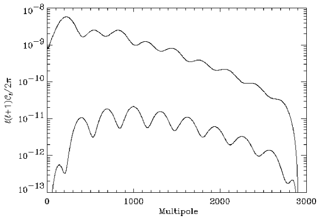
Figure 1: A typical angular power spectrum of temperature (upper line) and polarisation (lower line) anisotropy for a cold dark matter model with scale–invariant initial conditions. Only scalar fluctuations are considered.

2.4 Secondary Anisotropies

Different processes can generate anisotropy in the path from the LSS to the observer. Detailed observation of these effects provides insight on the evolution of the universe after recombination. A first effect is the Integrated Sachs-Wolfe effect (ISW; see Eq. (16)) generated by time variations of the gravitational potential in the photons’ trajectory. These time variations can be due to potential decay, gravitational waves (tensor perturbations) or non-linear effects associated to structure formation.

There are mainly three situations in which the potential time derivative is not zero and they give rise to the Early ISW, the Late ISW and the Rees-Sciama effect [37] respectively. Soon after recombination the photon density is not completely negligible and this causes $\Phi$ to decay producing the Early ISW effect which peaks slightly to the left of the first acustic peak. In open or $\Lambda$-dominated models, the universe eventually becomes curvature or vacuum dominated respectively. This produces a variation in $\Phi$ yielding the Late ISW effect since curvature and vacuum are important at low redshifts. This affects only very large angular scales. When structures begin to form, entering a non-linear regime, the approximation of constant $\Phi$ in time is no longer valid and variations in $\Phi$ cause the Rees-Sciama effect, relevant for the very small angular scales of the CMB power spectrum.

Another source of secondary anisotropy is gravitational lensing. While the ISW does change photon energy but not their directions from the potential gradient parallel to the photon path, gravitational lensing alters photon directions leaving, to first order, their energy unchanged. This is produced by the potential gradient perpendicular to the photons path. The effect on CMB angular power spectrum is a smoothing of the acoustic oscillations at large and intermediate scales, while it adds extra power at small angular scales [41] (ref. Martinez-Gonzalez).

All these are gravitational effects. Other processes producing secondary anisotropy are related to local and global re-ionisation of the universe. As for local re-ionisation, this is usually located in galaxy clusters and is called Sunyaev-Zel’dovich (S-Z) effect [42]. This is the result of the Compton scattering of the CMB photons by non-relativistic electron gas within clusters of galaxies (see [43] for an excellent review). This “thermal” effect, driven by the thermal motions of the electrons, results in a systematic shift of photons from the Rayleigh-Jeans to the Wien side of the frequency spectrum. With respect to the incident radiation field, the change of the CMB intensity across a cluster can be viewed as a net flux emanating from the cluster. The flux is negative below the characteristic frequency, $\nu_{0}=217\,$GHz, and positive above it. The change in the spectral intensity is given by:

$$\Delta I=\frac{(2kT_{0})^{3}}{(hc)^{2}}\frac{x^{4}e^{x}}{(e^{x}-1)^{2}}y\left[x{\rm coth}\frac{x}{2}-4\right]\ ,$$ (18)

where $x\equiv h\nu/kT_{0}$ is the dimension-less frequency and $y$ is the Comptonisation parameter:

$$y\equiv\frac{k\sigma_{T}}{m_{e}}\int dlT_{e}n_{e}\ ,$$ (19)

where $\sigma_{T}$ is the Thomson scattering cross section, $n_{e}$ and $T_{e}$ are the electron density and temperature, respectively, and the integral is computed along the line of sight.

An additional effect caused by scattering of CMB photons against electrons in bulk motion is the so-called “kinematic” S-Z effect. Its amplitude is proportional to the line of sight component of the peculiar velocity, $v_{r}$, and can then be used to determine clusters peculiar velocities [44, 45].

If the universe becomes globally re-ionised, the effect on CMB anisotropy is quite dramatic. The CMB is scattered by free electrons and photons we see coming from a given direction may instead be originated from a completely different direction on the LSS. This leads to a damping of anisotropies on scales smaller than the horizon size at the redshift of re-ionisation. If the universe become re-ionised at redshift $z_{r}$ and remained ionised up to now, the probability that a CMB photon never experienced a scattering is $e^{-\tau}$ where $\tau$ is the optical depth at re-ionisation. Since the power spectrum is the square of fluctuations, this probability becomes $e^{-2\tau}$. In a standard CDM universe $\tau$ becomes larger than 1, implying that almost all photons are scattered at $z_{r}\sim 50$ corresponding to scales smaller than few degrees. Therefore the larger $\ell$’s are suppressed by a factor $e^{-2\tau}$ while the low $\ell$’s are left unaffected.

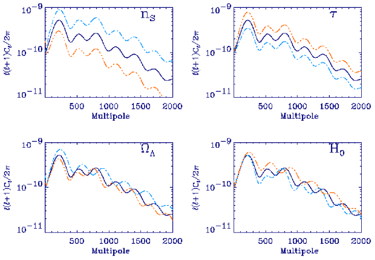
Figure 2: Examples of the dependence of the shape of the angular power spectrum $C_{\ell}$ on the value of the cosmological parameters. The fiducial power spectrum (solid line) is a model with $\Omega_{b}=0.05$, $\Omega_{\rm CDM}=0.35$, $\Omega_{\Lambda}=0.6$, $H_{0}=65$ km s^-1 Mpc^-1, $n_{S}=1.0$ and $\tau=0.3$. In each panel, all the parameters are unchanged except for the one indicated. The dash-dot-dot-dot line and the dash-dot line refer to values: $n_{S}=(0.8,1.2)$ (upper left); $\tau=(0.0,0.5)$ (upper right); $\Omega_{\Lambda}=(0.4,0.8)$ (lower left); and $H_{0}=(40,80)$ km s^-1 Mpc^-1 (lower right).

2.5 Dependence on cosmological parameters

We have seen that a number of processes contribute to the generation of CMB anisotropy field. Starting from such processes, the shapes, heights and locations of peaks and troughs in the angular power spectrum are predicted by all models which, like CDM, are based on the inflationary scenario. Furthermore the details of the acoustic features in the power spectrum depend critically on the chosen cosmological parameters [46, 47], which in turn can be accurately determined by a precise measurement of the anisotropy pattern. In this section we briefly discuss the sensitivity of the $C_{\ell}$’s on the value of some fundamental parameters (see Fig. 2).

• Total density: a decrease in $\Omega_{0}$ corresponds to a decrease in curvature and increase, although small, in Late ISW effect, with a corresponding shift of the power spectrum peaks towards high multipoles. In particular it can be shown that the angular scale of the first peak is $\ell_{1}\approx 200\sqrt{\Omega_{0}}$.

• Barion density: an increase in the baryon fraction $\Omega_{b}$ will increase odd peaks (compression phase of the baryon-photon fluid) due to extra-gravity from baryons with respect to the even peaks (rarefaction phase of the fluid oscillation).

• Hubble constant: a decrease in $h$ ($h\equiv H_{0}/100$ km s^-1 Mpc^-1), maintaining $\Omega_{b}h^{2}$ fixed at the nucleosynthesis value (typically $\Omega_{b}h^{2}=0.019\pm 0.002$, see [48]), corresponds to a delay in the epoch of matter radiation equality and to a different expansion rate; this boosts the peaks and slightly changes their location in $\ell$-space.

• Cosmological constant: an increase in the cosmological constant, $\Lambda$, in a flat space, again corresponds to a delay in matter-radiation equality with a boosting and shifting effect on the peaks. Furthermore the low $\ell$’s are affected by the Late ISW effect.

• Spectral index: increasing $n_{S}$ will raise the angular spectrum at large $\ell$’s with respect to the low $\ell$’s.

• Reionisation: if the intergalactic medium was re-ionised at $z\ll 1000$, then the power at $\ell>100$ would be suppressed by a factor of $e^{-2\tau}$. Evidence for early reionisation would set important constraints on theories of galaxy formation and on the epoch at which the first structures formed. A recent combined analysis [49] of CMB data and Large Scale Structure data together with Big Bang nucleosynthesis priors yields $\tau\simeq 0.1$.

• Gravitational wave background: gravitational waves (tensor modes) generate additional CMB anisotropies, but only at large angular scales. Inflationary models predict that the ratio of tensor to scalar contribution to the quadrupole anisotropy ($r=C^{(T)}_{2}/C^{(S)}_{2}$) is related to the spectral index of primordial tensor fluctuations, $n_{T}$.

As we shall see, present CMB anisotropy data already constrain significantly some of these parameters. However, much more accurate data are required to fully extract the cosmological information encoded in the CMB power spectrum.

2.6 CMB polarisation anisotropies

Theoretically, the degree of linear polarisation is directly related to the quadrupole anisotropy in the photons when they last scatter [50, 51, 52]. While the exact scale dependence of polarisation depends on the mechanism for producing the anisotropy, several general properties can be identified. In particular, the polarisation power spectrum peaks at angular scales smaller than the horizon at last scattering, since the processes that produce it are causal (see Fig. 1). Furthermore, the polarised fraction of the temperature anisotropy is small, since only those photons that last scattered in an optically thin region could have possessed a quadrupole anisotropy (multiple scattering causes photon trajectories to mix and hence erases anisotropy). This fraction, which depends on the duration of last scattering, is expected to be of  5-10% on a characteristic scale of tens of arcminutes.

CMB polarisation provides an important tool for reconstructing the model of the fluctuations from the observed power spectrum. In fact polarisation probes the epoch of last scattering directly, unlike the temperature fluctuations which may evolve between LSS and the present (see Sect. 2.4). This localisation in time is a very powerful tool for reconstructing the sources of anisotropy. Moreover, different sources of temperature anisotropies (scalar, vector and tensor) give different patterns in the polarisation, both in its intrinsic structure and in its correlation with the temperature fluctuations themselves.

Finally, the CMB polarisation power spectrum provides information complementary to the temperature power spectrum even for ordinary (scalar or density) perturbations. This can be of use in breaking degeneracies in the determination of the cosmological parameters, thus constraining them even more accurately [53].

3 ASTROPHYSICAL LIMITATIONS

In a CMB experiment, the measured signal contains many different contributions, beside the CMB, some of which are astrophysical (both galactic and extra-galactic) in origin. These astrophysical foreground emissions can be separated from the CMB up to a certain level of accuracy by means of multi-frequency measurements, although there is currently no emission component for which both angular and frequency destributions are precisely determined. Galactic and extragalactic microwave and sub-mm emission, while representing a challenge for CMB experiments, yield by themselves interesting astrophysical information.

3.1 Galactic synchrotron emission

Diffuse Galactic synchrotron emission originates from cosmic-ray electrons accelerated in the Galactic magnetic field. Therefore the intensity of this emission depends on the energy distribution of electrons as well as on the structure of the Galactic magnetic field (see [54] for a recent review). Synchrotron radiation dominates at frequencies $\nu\,\lower 2.0pt\hbox{${<\atop\hbox{\raise 4.0pt\hbox{$\sim$}}}$}\,10$ GHz which makes it possible to obtain, in this frequency range, sky maps of genuine synchrotron radiation. Large sky area surveys, however, suffer significant uncertainties associated with calibration errors, zero levels and scanning strategy artifacts. At frequencies below 1 GHz instrument gain and zero-level uncertainty are considerably smaller than the observed signal and reliable sky maps have been obtained at 408 MHz [55] over the whole sky, and at 1420 MHz [56] and 2326 MHz [57] over large sky fraction. The typical angular resolution of these surveys is $0.85^{\circ}\div 0.3^{\circ}$.

The synchrotron brightness temperature is expected to scale with frequency as a power law, $T_{b}\propto\nu^{-\beta}$, with a spectral index $\beta$ which vary with frequency and position according to the energy distribution of electrons and Galactic magnetic field structure. The mean temperature brightness spectral index between 38 and 1420 MHz is $\beta\simeq 2.7$ with variations of at least 0.3 and the de-striped 408 and 1420 MHz maps gave temperature spectral indices of 2.8 to 3.2 in the northern galactic pole regions [58]. Some evidence of a high frequency steepening of $\beta$ was reported [59] considering data taken from the White Mountain site [60] with $18^{\circ}$ angular resolution together with 408 and 1420 MHz maps to estimate the spectral index between 1 and 10 GHz. A mean value of $\beta=2.76\pm 0.11$ has been found.

As for the angular dependence of synchrotron emission there is not a general agreement. Some authors [61] suggested that synchrotron angular power spectrum should scale as $\ell^{-3}$ as observed for dust emission. However other authors [62] considering the region observed by the Tenerife experiment (see Sect. 7.2.4) found a rather low amplitude as well as a flatter angular dependence ($\ell^{-2}$).

Synchrotron radiation is expected to be polarised by a large fraction (in principle up to $\sim$ 70%). This could be a problem in CMB polarisation measurement since the CMB polarised signal is expected at the few $\mu$K level. Furthermore, the spectral behaviour of synchrotron polarised emission as well as its angular dependence are not known. Detailed studies exploiting the small database of polarisation measurements available are currently on-going [63].

3.2 Galactic free-free emission

When a free electron is accelerated by the Coulomb field of ions, free-free emission results. This occurs when hot electrons ($T_{e}\,\lower 2.0pt\hbox{${>\atop\hbox{\raise 4.0pt\hbox{$\sim$}}}$}\,10^{4}$ K) interact with an ion, starting from an un-bound state and ending, after interaction, in another un-bound state. The physics of this process is well know. It is possible to calculate the emissivity per volume along the line of sight of a given distribution of electrons. When integrating the emissivity we obtain the optical depth and then the brightness temperature which scales as:

$$T_{b}^{ff}\sim 26\,\mu{\rm K}\,\,\,\nu^{-2.1}T_{e}^{-0.35}\ EM\ ,$$ (20)

where $T_{e}$ is the electron temperature and $EM\equiv\int N_{i}N_{e}dl$ is the emission measure which depends on the number of ions, $N_{i}$, and electrons, $N_{e}$, per unit volume. Due to the harder spectrum with respect to synchrotron emission, free-free should dominate the microwave sky at frequencies $\nu\,\lower 2.0pt\hbox{${>\atop\hbox{\raise 4.0pt\hbox{$\sim$}}}$}\,10$ GHz. However, the signals are extremely weak and no sky survey of free-free emission free of other components is available.

Free-free emission arises from two distinct components, one discrete and one diffuse. The former is clearly associated with Hii regions. These are regions of intense star formation where hot electrons are present. They are mainly localised along the galactic plane ($|b|<5^{\circ}$) with very few exceptions (e.g. the Orion Nebula). In a recent work [64] a catalogue of about $\sim 1200$ Hii regions at 2.7 GHz has been produced. Since free-free emission is expected not to be polarised, Hii regions could be used to separate instrumental polarised components in CMB measurements at sub-degree angular resolution.

As for the diffuse component, we have to rely on tracers of the ionised interstellar medium. Most of the available information at intermediate and high latitudes comes from H$\alpha$ surveys from which it is possible to derive the free-free brightness temperature:

$$T_{b}^{ff}\sim 1.68\mu{\rm K}\langle g_{ff}\rangle T^{0.4\ {\rm to}0.7}\lambda I_{H\alpha}\ ,$$ (21)

where $\lambda$ is in cm, $I_{H\alpha}$ is the intensity of the H$\alpha$ emission and $\langle g_{ff}\rangle$ is the Gaunt factor. Therefore a measurement of H$\alpha$ emission directly yields microwave free-free brightness temperature.

A correlation between free-free and dust emission was found [65] comparing the $COBE$-DMR maps with the DIRBE maps. Modelling the emission as combination of dust and radio components, a radio spectral index $\beta_{\rm radio}\simeq-2.1^{+0.6}_{-0.8}$ was determined in good agreement with the expected index of free-free emission (Eq. (20)). This was later confirmed [66, 67] down to 14 GHz with a spectral index consistent with free-free emission at 95% confidence level. However the microwave emission reported in [66, 67] is 5-10 times larger than derived from H$\alpha$ measurements in the same regions [68]. This is quite interesting: microwave emission is correlated with dust showing a spectral index consistent with free-free but the H$\alpha$ emission cannot account for the overall emission observed. Recently [69] a possible explanation of this “anomalous” emission was suggested, invoking the contribution from electric and magnetic dipole from small spinning dust grains. This emission should in fact peak between 10 and 50 GHz, and it would explain the observed correlation with dust emission as well as the lack of H$\alpha$ emission. More multi-frequency measurements are required to clarify the issue.

As for the spatial behaviour of free-free emission [65] at angular scales $>7^{\circ}$ the angular spectral index was estimated $\simeq 3.0$, a well-determined value for dust and HI at degree scales. This was confirmed to some extent [67] for the North Celestial Pole (NCP) region in a correlation of Saskatoon data (see Sect. 7.2.7) with the IRAS and DIRBE maps.

3.3 Galactic dust

Galactic dust emission originates from dust grains heated by interstellar radiation: dust absorbs UV and optical photons and re-emits in the far-IR. Dust emission typically dominates at $\nu\,\lower 2.0pt\hbox{${>\atop\hbox{\raise 4.0pt\hbox{$\sim$}}}$}\,100$ GHz and the total intensity depends upon gas chemical composition, dust to gas ratio and grain composition, structure and dimension.

The spectral shape of dust emission can be well modelled by a modified blackbody emissivity law $I_{\nu}\propto\nu^{\alpha}B_{\nu}(T_{d})$ where $\alpha\simeq 2$ is the emissivity, $T_{d}$ is the dust temperature and $B_{\nu}(T)$ is the planckian function. Exploiting $COBE$-DIRBE data and focussing on high galactic latitude regions, a dust temperature of 18 K has been found [65]. More recently a dust emission map obtained by joining together the $COBE$-DIRBE and the IRAS maps with IRAS angular resolution ($\sim 6^{\prime}$) has been produced [70]. A best fit model with two dust temperature (16 and 9.5 K) and two distinct emissivities (2.7 and 1.7 respectively) was proposed based on exploiting the $COBE$-FIRAS data in the range between 100 and 2100 GHz.

The analysis of dust contamination is further complicated by the highly non-Gaussian nature of its Galactic distribution. The new Berkeley-Durham dust map [70] shows that its power spectrum is not well described by a global $\ell^{-3}$ power law everywhere at high Galactic latitude, as it was claimed [71]; in some high galactic latitude patches the power spectra are closer to $\ell^{-2.5}$, but with amplitudes differing from patch to patch.

3.4 Extragalactic sources

Beyond galactic foregrounds, another unavoidable fundamental limitation for CMB measurements come from extra-galactic sources that are expected to be a significant challenge for future high-resolution CMB experiments. The issue of small scale fluctuations due to extra-galactic sources has been long discussed in literature (e.g. [72, 61]). Due to the sharp rise in the dust spectrum with increasing frequency ($\propto\nu^{3.5}$) different populations of bright sources below and above 200 GHz show up. Radio sources (“flat”-spectrum radio-galaxies, BL Lacs objects, blazars and quasars) dominate at low frequencies while dusty galaxies strongly contribute at high frequencies.

The large uncertainties on number of counts and spectra for radio sources do not allow a comprehensive model of source counts at $\sim 100$ GHz, although simple models [73, 74] seem to be remarkably successful, as they properly account for deep counts at 8.44 GHz recently produced. The situation for dusty galaxies is more complicated since evolutionary properties are poorly known and source counts are strongly evolution sensitive. The situation is however improving with the ISO-CAM, ISO-PHOT and SCUBA data [75] although limited to small sky areas. Number of counts for both radio and dusty galaxies has been studied in the context of the Planck mission [73] showing that at 5$\sigma$ level several hundreds of sources will be detected at each frequency channel.

Even assuming that the resolved sources can be completely removed, we are left with the background of the un-resolved ones. A Poisson distribution over the whole sky would produce a simple white-noise power spectrum, with the same power in all multipoles $\ell$, so that it dominates cosmic signal on small scales. For radio point sources [73] the level for the power spectrum is found to be:

$$\sqrt{\ell(\ell+1)C_{\ell}/2\pi}\simeq\frac{{\rm sinh}^{2}(\frac{\nu}{113.6})}{(\nu/1.5)^{4.75-0.185{\rm log}(\nu/1.5)}}\ell\ ,$$ (22)

where $C_{\ell}$ has units of K² and $\nu$ is expressed in GHz. The point source contribution is well below the level of CMB fluctuations in the range $50\div 200$ GHz at angular scales larger than few arcminutes. Source clustering would add some power on larger scales; however, its contribution is found to be generally small in comparison with the Poisson term [73].

Fig. 3 summarises the relative importance of galactic and extra-galactic foreground fluctuations with respect to CMB anisotropy as a function of frequency for different angular scales and galactic cuts. In all cases, the combination of foreground fluctuations in the range 70-100 GHz is at least an order of magnitude below the typical CMB anisotropy. While this shows that, with proper choice of frequency, foregrounds do not represent a severe limitation to first-order statistical studies, it is also clear that, to separate components at  1% level, a careful multi-frequency approach of instrument design and data analysis is mandatory.

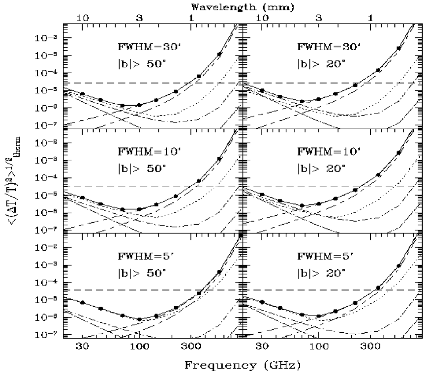
Figure 3: Temperature fluctuations for three different angular resolutions and two different cuts in galactic emission, as a function of frequency. The horizontal dashed line is the expected level of CMB fluctuations from a standard CDM model. Dot-short dashed, dot-long dashed and long-short dashed represent the mean contribution from Galactic free-free, synchrotron and dust emission respectively. Lower long/short dashed is a lower limit for Galactic dust fluctuations. The dotted curves represent the contribution from extra-galactic point sources fainter than 100 mJy [73]. The solid curve is the quadratic sum of all the contributions and the filled circles are the selected Planck frequencies. From De Zotti et al.[76]

.

4 OBSERVATIONAL ISSUES

Following the $COBE$-DMR first detection [15], observations of the CMB anisotropy have experienced a time of explosion. At present, as many as 70 papers report positive detection of $\Delta T/T$ at a variety of angular scales and with different observing techniques. Here we present some general issues relevant to CMB anisotropy experiments, related to the observing strategy, design and technical features which ultimately impact on the final precision in the measurement.

4.1 Cosmic and sample variance

The “cosmic variance” sets the ultimate limit on the accuracy of our estimates of the power spectrum. In most theories the CMB field is a single realisation of a stochastic process, and we should not expect our observable universe to follow exactly the average over the ensemble of possible realisations. This is equivalent to say that the $a_{\ell m}$ coefficients are independent identically distributed Gaussian random variables (for a given $\ell$) and therefore the $C_{\ell}$ are a $\chi^{2}$ distribution with $2\ell+1$ degrees of freedom. The variance in $C_{\ell}$ is then:

$$\frac{\Delta C_{\ell}}{C_{\ell}}=\sqrt{\frac{2}{2\ell+1}}\ ,$$ (23)

which is quite important at low $\ell$ since a small number of modes ($m=2\ell+1$) is available.

Similarly, incomplete sky coverage degrades the accuracy on $C_{\ell}$ since the observed region of the sky may not be representative of the realisation as a whole. For experiments which do not cover the full sky, this “sample variance” is larger than the cosmic variance by a factor proportional to the inverse of the fraction of the sky surveyed.

4.2 Window functions and observing strategy

The experiment window function $W_{\ell}$ is determined by the instrument beam and sky scanning technique, and selects the angular range at which the measurements are sensitive. Typical beam switch experiments have $W_{\ell}$ peaking in a relatively narrow range of the corresponding scales of the power spectrum [77]. Early measurements were designed to sparsely sample the autocorrelation function at a fixed angular scale. On the other hand, to obtain a model–free reconstruction of the power spectrum one needs a function $W_{\ell}$ nearly constant over a range of angular scales as wide as possible. This is the characteristic of an imaging observation [78], where several different angular scales are simultaneously probed. Interferometry and arrays of radiometers or bolometers with proper sky scanning strategy, as we shall see, can both obtain images of large areas of the sky with adequate sensitivity.

The sky power averaged over the region observed with a beam characterised by a window function $W_{\ell}$ can be written as:

$$\left(\frac{\Delta T}{T}\right)_{rms}^{2}=\sum_{\ell}\frac{2\ell+1}{4\pi}C_{\ell}W_{\ell}$$ (24)

which is in fact the convolution of the sky power with the function $W_{\ell}$. The most simplest window function is that of a single Gaussian beam of width $\sigma_{B}$ (related to beam Full Width Half Maximum by FWHM = $\sigma_{B}2\sqrt{2{\rm ln}2}$) for a full sky coverage:

$$W_{\ell}={\rm exp}[-\ell(\ell+1)\sigma_{B}^{2}]\ .$$ (25)

Note the high-$\ell$ cut-off due to finite angular resolution, which occurs at $\ell_{\rm cutoff}\cong 1/\sigma_{B}$. If we consider an experiment that measures temperatures by chopping between 2 or 3 beams in the sky, the window function has additional terms:

$${\rm exp}[\ell(\ell+1)\sigma_{B}^{2}]\ W_{\ell}=\bigg{\{}\begin{array}[]{lr}2[1-P_{\ell}({\rm cos}\ \theta_{c})]&{\rm 2-beam}\\ 1/2[3-4P_{\ell}({\rm cos}\ \theta_{c})+P_{\ell}({\rm cos}\ 2\theta_{c})]&{\rm 3-beam}\\ \end{array}$$ (26)

where $P_{\ell}$ are the Legendre polynomial and $\theta_{c}$ is the chopping angle. These observing strategies introduce a low-$\ell$ cut-off. More generally $W_{\ell}$ is the diagonal part of the window function matrix $W_{\ell\ell^{\prime}}$ which takes into account the coupling between different multipoles $\ell$ due to the observational strategy and to the non-orthogonality of the spherical harmonics on a limited region of the sky (in general observed by a multiple beam switch experiment).

The knowledge of the window function is extremely important when comparing results from different experiments. It is usual to represent power spectrum data in terms of $(\Delta T/T)_{\ell}^{2}\equiv\ell(\ell+1)C_{\ell}/2\pi$ (band-power). Therefore from the measured $(\Delta T/T)_{\rm rms}^{2}$ and using the expression (from Eq. (24)):

$$\left(\frac{\Delta T}{T}\right)_{\rm rms}^{2}=\left(\frac{\Delta T}{T}\right)^{2}_{\ell}\sum_{\ell}W_{\ell}\frac{2\ell+1}{2\ell(\ell+1)}\ ,$$ (27)

it is possible to obtain $(\Delta T/T)_{\ell}$.

4.3 Instrument related variance

Detector sensitivity and angular resolution are key performance parameters. Combining cosmic, sample and instrumental effects, the final fractional error on the $C_{\ell}$’s can be written as follows [79]:

$$\frac{\delta C_{\ell}}{C_{\ell}}=\sqrt{\frac{2}{{f_{\rm sky}(2\ell+1)}}}\bigg{[}1+\frac{A\sigma^{2}}{NC_{\ell}W_{\ell}}\bigg{]}\,,$$ (28)

where $f_{\rm sky}$ is the fraction of the sky surveyed, $A$ is the physical dimension of the surveyed area, $\sigma$ is the rms noise per pixel and $N$ is the number of observed pixels.

We will discuss in some detailed the issue of sensitivity and how technically this is addressed in Sect. 4.7. As for the angular resolution, we note here that the FWHM of microwave horns are limited to $>5^{\circ}$-$6^{\circ}$, which probes the power spectrum only to $\ell\lesssim$ 20; as a consequence, to perform sub-degree scale measurements either interferometry techniques or the use of a telescope is required. Interferometers can achieve arcminute angular resolutions at cm wavelengths, while telescopes need a primary reflector with an aperture $D\approx\theta_{\rm FWHM}\lambda\approx$ 1 to 2 meters to reach $\sim$ 0.5^∘. Generally, Gregorian or Cassegrain off-axis, clear-aperture optical systems are employed to minimise diffraction from the sub-reflector and from the support structure. Detailed shaping of the reflector surface may be used to minimise beam aberration. We will discuss issue related to optical effects in Sect. 5.1 and 5.2.

4.4 Atmosphere

The radiation coming from the earth environment represents one of the main problems for sub-orbital experiments, because it adds a background which varies both in time and direction. The uncertainty in the atmospheric contribution in turn affects the capability of removing astrophysical foregrounds in the analysis. While it has been proven that ground–based experiments can produce high quality CMB anisotropy data, it is unlikely that atmospheric noise can be rejected or removed to the levels required to accurately subtract the galactic foregrounds on large portions of the sky.

The atmosphere emits and absorbs radiation in a complicated way, which depends on wavelength, pressure, temperature and chemical composition, with O₂, O₃ and H₂O as the the most important microwave-emitting molecules [80]. Three spectral windows ($<$ 15 GHz, 30-40 GHz, 85-110 GHz) of the microwave atmospheric spectrum are exploited by ground-based measurements usually taking advantage of the optimal performance in this frequency range of coherent receivers.

The impact of atmospheric radiation largely depends on the variability of the water vapour content. For this reason ground-based experiments are usually located in dry high altitude sites. For example, the Izana site at Tenerife, Canary Islands [81, 82] has a typical water vapour column of $\sim 2$ mm and atmospheric antenna temperature $T_{A}\sim 4.7$ K and $T_{A}\sim 8.7$ K at $28$ and $38$ GHz, respectively. The Antartic Plateau is possibly the best ground-based site in terms of atmospheric emission and stability [83, 84]. At the South Pole, at 30 GHz, the atmospheric emission amounts to $T_{A}\sim 4.6$ K, with only 0.15 K contributed by water vapour (0.5 mm H₂O column), and the atmospheric noise is at a level of $3\times 10^{-6}$ $T_{A}$. The impact of atmospheric noise on the data also strongly depends on the instrument concept and scanning technique, and it is particularly well suppressed in interferometer experiments. In addition to water vapour fluctuations, pressure gradients in the observed sky patches are likely to induce significant large-scale variations of the O₂ emission, as direct measurements from the South Pole site have shown [85].

For balloon-borne experiments the overall signal from the atmosphere is reduced by two to three orders of magnitude depending on frequency. The reduced pressure yields a lower pressure broadening of lines which are now clearly visible. The effects of the atmosphere are strongly reduced (although not suppressed) so that high–frequency measurements ($100<\nu<500$ GHz) can be performed. Only for a space mission is the whole frequency range available with no limitations other than the unavoidable galactic and extragalactic emission.

4.5 Ground Radiation

Due to the large solid angle of the earth compared to the beam angular resolution (say $\sim 0.5^{\circ}$), for a ground–based experiment seeking final accuracies $\Delta T/T\sim$ $10^{-6}$, the unwanted signal from the ground needs to be rejected by a factor as high as 10¹³ to fall below significance level. For anisotropy experiments one is concerned only with the level of the variable component of ground contamination from pixel to pixel, which can be made, say, 1000 times smaller than the total ground contribution; even in this assumption (quite optimistic for large sky coverage experiments), the requirement of $\sim-100$ dB rejection is still extremely tight, and it becomes proportionally tighter moving to higher angular resolutions. From balloon altitudes, since the distance of the gondola from the earth is negligible compared to the earth radius, the sidelobe and straylight rejection required is of the same order as for ground-based experiments. A space mission from a low–earth orbit would only marginally relax such extreme requirement, since the earth would still cover about $1/4$ of the total solid angle. In fact, microwave emission from the earth has been a serious concern in the design and systematic error analysis of the $COBE$–DMR experiment, even at the relatively broad beams ($7^{\circ}$) of its antennas [86]. From the $COBE$ 900 km circular orbit, the earth is a circular source with angular diameter 122^∘ and minimum temperature 285 K. Upper limits to the antenna temperature of the earth signal contribution to the DMR 2–years data were at level 25–60 $\mu$K [87].

Clearly rejection of earth radiation is a major challenge to balloon–borne or low–earth orbit experiments aiming to reach sensitivities a factor $\sim$ 10 better than $COBE$–DMR with beam areas smaller by a factor of $\sim$100 to $\sim$1000. Only by moving the instruments to a far–earth orbit, is the earth’s solid angle greatly reduced, thus decreasing by the same factor the required rejection. Orbits around the sun-earth libration point L2 ($\sim 1,500,000$ km from earth) have been selected for both $MAP$ and Planck. The required rejection for earth radiation becomes comparable to that required to suppress sun radiation ($\simeq 10^{9}$), a level that can be obtained (and tested) with careful, though conventional design of the optics and shielding. We will come back to the more general issue of off-axis straylight in Sect. 5.2.

4.6 Calibration

The radiation power collected by a generic CMB detector is converted into a voltage $V$ that needs to be calibrated in physical units. Calibration is typically in terms of antenna temperature, $T_{A}\equiv P/k\Delta\nu$, proportional to the power received $P$ per unit bandwidth $\Delta\nu$. For a linear system $T_{A}=GV+T_{\rm offset}$, where $T_{\rm offset}$ is an instrument (constant) offset term. By observing two sources of known antenna temperatures $T_{A,1}$ and $T_{A,2}$, the calibration constant $G$ is readily determined as $G=(T_{A,1}-T_{A,2})/(V_{1}-V_{2})$. Although in principle $G$ is a constant characteristic of the receiver, in practice it undergoes drifts and time fluctuations. Thus good calibration requires well known, stable sources with adequate flux levels, to be observed at time intervals short compared to the variation of $G$.

Controlled blackbody targets at liquid He or N temperatures and suitable celestial sources are typically adopted. Jupiter, Mars, Saturn and Venus provide signals at $\sim 10$ to $100$ mK in a $\sim 10^{\prime}$ beam at mm wavelengths, a level adequate for calibration as well as for main beam mapping. Uranus and Neptune are also detectable sources with lower signal level (few hundred $\mu$K). The accuracy of planet calibration is limited to $3$-$10\%$ by the uncertainty in their brightness temperature in the microwaves (e.g. [88]). Experiments at degree scales also use the moon as a calibration source. Occasionally strong radio sources are employed, such as Cas A, Carina Nebula, Tau A. It may also be possible to use bright Hii regions, which however are often found in complex fields in the galactic plane, and beam pattern effects must be carefully separated [64].

For experiments covering significant sky areas with appropriate scanning strategies and at frequencies below $\sim 300$ GHz, a nearly ideal celestial calibrator is the CMB dipole: its amplitude ($\Delta T_{D}\sim$ 3.37 mK) and distribution are extremely well known [89, 8] and allow for countinuous observation. Furthermore, the dipole has the same frequency spectrum of the signal to be measured, i.e. the CMB itself. Balloon experiments like Boomerang and Maxima (see Sect. 7.3.7 and 7.3.8) achieved a few percent calibration accuracy using the dipole. Crosscheck with an independent source is a desirable strategy. For example, Boomerang also used an internal calibrator based on a germanium lamp with a well known signal amplitude and temporal profile [90]. At frequencies $>300$ GHz the Galactic plane as measured by FIRAS can be conveniently used.

The $MAP$ and Planck missions will fully exploit the CMB dipole for calibration. When high precision is required ($<1\%$), both instrumental and astrophysical effects must be carfully considered in the process. In particular, foregrounds emission from poorly known components add to the CMB dipole and can introduce systematic calibration discrepancies. It has been shown [91] that instroducing a frequency-dependent weight function allows to optimise the procedure. As for the $COBE$–DMR experiment [92], both missions can exploit the $\sim 0.3$ mK modulation of the CMB dipole in the 6-months period due to the seasonal velocity of the earth around the sun [93].

4.7 Technology

The $\Delta T/T$ detection by $COBE$-DMR used coherent microwave technology [94] in the frequency range 30-90 GHz; soon after that, the FIRS balloon survey confirmed the detection of cosmic structure with a bolometer receiver [95, 96] operating at 170-680 GHz. Both radiometer and bolometric detector technologies, after opening up the field of CMB anisotropy, have rapidly and continuously evolved up to now, and both have contributed to the dramatic progress in the past decade. The two technologies are optimally employed roughly below and above $\sim 100$ GHz, respectively.

4.7.1 Coherent receivers

Low system noise temperature $T_{\rm sys}$, large bandwidth $\Delta\nu$, and good stability are the key features for high performance radiometer. The minimum detectable temperature variation (sensitivity) of a receiver is:

$$\Delta T(f)=k_{R}T_{\rm sys}\sqrt{{1\over\Delta\nu\tau}+\left({\delta G(f)\over G}\right)^{2}}\,,$$ (29)

where $k_{R}\approx 1$ is a constant depending on the radiometer scheme [97], $\tau$ is integration time, and $\delta G(f)/G$ represents the contribution from amplifier gain and noise temperature fluctuations at post-detection sampling frequency $f$. Cooling of the first stages of amplification (typically to $\sim 100$ or $\sim 20$ K) is commonly used to reduce $T_{\rm sys}$, and low-loss ($\sim 0.1\div 0.5$ dB) wide band ($\delta\nu/\nu\sim$ $10\%\div 20\%$) front-end passive components (such as feed-horns, transition, couplers, orthomode transducers) are needed. Typically, the noise temperature of current state-of-the-art low noise transistor amplifiers exhibit a factor of 4–5 reduction going from 300 K to 100 K operating temperature, and another factor $2\div 2.5$ from 100 K to 20 K. Amplifier fluctuations exhibit a characteristic power spectrum $1/f^{\gamma}$ with $\gamma\approx 1$, i.e.

$$\Delta T(f)\simeq T_{\rm sys}\alpha\sqrt{1+{f_{\rm k}\over f}}\,,$$ (30)

where $\alpha$ is a normalised amplitude of the noise at high post-detection frequencies (i.e. in the pure white noise limit), and $f_{\rm k}$, called knee-frequency, is the frequency at which the white noise and $1/f$ components give equal contributions to the power spectrum. In HEMT devices $1/f$ noise is related to the presence of traps in the semiconductor [98]. As discussed in Sect. 5.4, $1/f$ noise not only degrades the sensitivity, but it may also introduce spurious correlations in the time ordered data and sky maps. To minimise these effects, it is common to design the instrument so that it takes differences between two nearly equal signals, which may be the sky and a stable reference termination, or two sky signals. The detected output of the radiometer can then be synchronously demodulated to produce data stable on time scales long compared to the switch period. A number of differencing schemes have been adopted, including the classic Dicke-switched scheme [99], correlation designs [100], and their combination with various beam switching schemes [101]. Continuous-comparison designs have been used at decimetre wavelengths [102, 103, 104]; more recently this technique was extended to higher frequencies thanks to improved manufacturing and low-loss performance of millimetre waveguide components [105]. Beam switching strategies, in which the beam is moved in the sky at a few Hz by a wobbling or rotating reflector, have been extensively adopted, sometimes in combination with total power receivers [106].

In recent years, high electron mobility transistor (HEMT) amplifiers have been widely and successfully employed both in differential receivers and interferometers at frequencies up to 90 GHz. These devices display a unique combination of features, including very low noise performance, wide bandwidth, operability at cryogenic temperatures and very low power consumption. The current generation of HEMT amplifiers is based on indium phosphide (AlInAs/GaInAs/InP heterostructure) which yields better noise performances and lower power consumption than the more traditional gallium arsenide technology (see, e.g., [107]). Recent progress in cryogenic HEMT noise temperature has been quite dramatic. In the late 70’s the advances in gallium arsenide field-effect transistors, combined with cryogenic cooling, made their noise performances competitive with parametric amplifiers [108]. In the past decade, further major improvements have been obtained, leading in the mid 90’s to state-of-the-art noise temperatures of 15 K at 40-50 GHz and 50 K at 60-75 GHz [109, 110, 111]. Today, the best measured performances are roughly a factor of 2 better (Sect.8.3.2). Receivers based on SIS (Superconductor–Insulator–Superconductor) junctions cooled to 4 K are capable of quantum limited detection, and are competitive with HEMTs [112] in the millimetre regime (e.g. in the $\lambda\simeq 3$ mm atmospheric window); however, they are now strongly limited in bandwidth [113, 114].

Corrugated feed horns are used to couple receivers with the sky or optical system (see, e.g., [115]), and very low sidelobe levels (down to $-90$ dB [116]) have been demonstrated. Designs optimised for good primary illumination and low edge taper include double profiled feeds [117, 118], for which high performances have been demonstrated at high frequencies [119].

4.7.2 Bolometric detectors

Bolometers are thermal detectors in which incoming photons give raise to phonons, and the temperature changes of the absorber is measured by a thermometer, typically doped silicon or germanium [120]. The resistance $R$ of the thermometer changes with its temperature, which can be measured by applying a constant current. The typical application of bolometers in astrophysics is in the sub-mm range (0.2$<\lambda<$3 mm), although they are also used in a variety of regimes, including X-ray.

A semi-empirical formula [121] describes the bolometer sensitivity in terms of noise equivalent power ($NEP$) as:

$$NEP^{2}={2kT_{0}\over\pi}(f_{0}CT_{p})\left({9\over A}+{25\over A^{2}}\right)+4kT_{0}{36W_{0}\over A}\,,$$ (31)

where $T_{p}$ is physical temperature, $f_{0}$ is frequency response, $C$ is the material’s heat capacity, $W_{0}$ is the steady component of the optical power, and $A$ is given by:

$$A=-{d{\rm Log}R\over d{\rm Log}T}\approx 3.$$ (32)

It is clear that reducing $T_{p}$, which controls both the first and second terms in equation (31), one can in principle reach extreme sensitivity. It can be shown that the critical temperature below which the bolometer $NEP$ is limited by unavoidable photon noise [122] for a source with blackbody temperature $T_{S}$ given by:

$$T_{p}<{1\over 18}AT_{S}\,.$$ (33)

In the case of CMB observations, $T_{S}\approx 3$ K, so that the critical temperature is $T_{p}\approx 0.5$ K. Current state-of-the-art bolometer technology, combined with the sophisticated cryogenic chains needed to reach the extremely low temperatures (typically $0.3$ K to $0.1$ K) required, allows to reach photon-noise-limited sensitivity.

Unlike coherent detectors, bolometers are sensitive to radiation from any frequency and any direction. The absorber is normally housed in a cavity which enhances the bolometer efficiency by multiple reflection of the radiation. Coupling of the detector to the telescope is achieved with either multimode concentrators, such as Winston cones, or with single-mode corrugated feedhorns (now preferred at least for frequencies $<300$ GHz). To avoid self-emission, the front-end temperatures must be kept as low as possible. Frequency selection is achieved with high-efficiency filters (typically rejecting out-of-band radiation at $10^{-9}$ level). These are cooled down enough to avoid stray emission towards the bolometers, but at the same time they must be compatible with the system cooling power.

A recent breakthrough in bolometer technology has been achieved with the introduction of “spider-web bolometers”, first development at the JPL Center for Space Microelectronics Technology [123, 124], with silicon nitride (Si₄N₃) micromesh. In this technique, a resistive grid is used to absorb the radiation, instead of a continuous metallic layer. These bolometers have better sensitivity due to the reduction of the heat capacity $C$ of the absorber (see equation (31)). In addition, the web structure reduces the detector mass by two orders of magnitude thus decreasing the bolometer’s sensitivity to microphonics. Also, its smaller cross-section reduces dramatically the importance of cosmic rays hits as well as of high frequency radiation. Noise equivalent power of order $10^{-17}$ W$\times$Hz^-1/2 have been measured.

5 INSTRUMENTAL SYSTEMATIC EFFECTS

Possibly the most challenging aspect in CMB experiments is the need to reject and control all possible systematic effects. While this is true for any experiment, the importance of systematic effects is exacerbated in situations where the sought-for signal is embedded in the noise, thus requiring long integration times. When the goal is a mere “detection” of the CMB anisotropy one can reasonably plan the rejection of spurious signals at $\sim 30\%$ of the CMB anisotropy, or $\sim$15-30 $\mu$K level. However, in the present era of transition to precision measurements, experimenters require control of systematics 10 times better, or $\sim$1-3 $\mu$K level. High resolution CMB measurements at sensitivity $\Delta T/T\approx 10^{-6}$ thus require an environment and viewing field extremely free from local contamination. Instruments must be designed with the aim to control in hardware the level of systematic effects introduced in the measured data: experience has demonstrated that the more and the larger are systematic effects which have to be removed in the data analysis, the less robust the final result will be.

5.1 Optical effects. Main beam distortions

The observed signal is the result of the convolution of the antenna beam pattern with the sky signal distribution (expressed in antenna temperature):

$$T_{\rm A}(\theta_{0},\phi_{0})=\frac{\int d\Omega P_{n}(\theta-\theta_{0},\phi-\phi_{0})T_{\rm sky}(\theta,\phi)}{\int d\Omega P_{n}(\theta,\phi)}\,,$$ (34)

where $T_{\rm sky}(\theta,\phi)$ is the sky temperature in the direction $(\theta,\phi)$ and $P_{n}(\theta,\phi)$ is the normalised antenna beam pattern. Ideally, the beam is a pure symmetric Gaussian in shape. In practice non-idealities occur in the $P_{n}(\theta,\phi)$ function. The effects on $P_{n}(\theta,\phi)$ in its very central part are usually called main beam distortions; the signal coming from secondary lobes is instead referred to as stray-light signal. Fig. 4 shows a typical simulated beam at 100 GHz for the Planck-LFI instrument: the beam pattern is quite symmetric down to -10 $\div$ -20 dB while at lower level several structures appear. The contour at -10 dB shows also a slight deviation from a perfect circle.

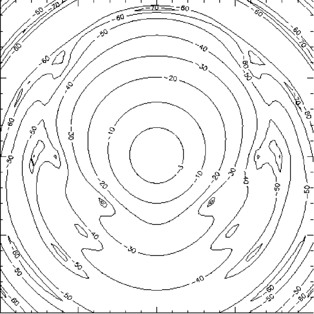
Figure 4: Typical simulated beam pattern at 100 GHz for the Planck-LFI instrument. Courtesy of F. Villa.

Optical aberrations make the main beam (within few FWHM from the beam centre) different from the ideal reference case of a pure centrally symmetric Gaussian shape. Main beam distortions may introduce a degradation of the angular resolution and of the sensitivity per resolution element. These two effects can be seen as orthogonal in the $\theta-\Delta T$ space of angular scales and temperature anisotropy or, equivalently, in the $\ell-C_{\ell}$ space [125]. The net effect is lowering the maximum multipole $\ell$ probed and increasing the error on $C_{\ell}$.

The need for multi-frequency, high sensitivity and high angular resolution in present and future CMB experiments calls for a multi-frequency focal plane arrays placed at the focus of an optical system. As a consequence, the detectors located far from the optical axis will suffer more beam distortion effects. While sophisticated optical shaping can be optimised to use a large focal area [126, 127], this effect can be a limiting factor in the growth of array size.

5.2 Optical effects. Side-lobe radiation

The radiation pattern at large angles from the main beam (sidelobes) is due to diffraction and scattering effects from the edge of the mirrors as well as from the nearby supporting structures (see Fig. 5). In Sect. 4.5 we discussed the issue of sidelobe effects from earth radiation. Of course the problem is much more general. The source of stray-light may be both internal to the instrument, e.g. emission from the telescope; and external, i.e. from the surrounding environment, from small solid angle sources like sun, moon, planets, or from diffuse sources like the Galactic plane. The amplitude of the effect can be reduced by decreasing the edge taper by design of the feed, at the cost of loss in angular resolution. The level of stray-light depends on the orientation of the beam profile with respect to external and internal sources.

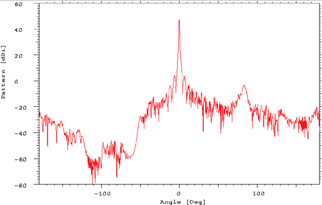
Figure 5: Cut of a simulated Planck-LFI beam profile at 30 GHz. A part from the main beam, several other features are present due to diffraction of the telescope, shield and supporting structures. The integrated power of the beam profile is dominated by the main beam ($\approx$ 98%) and the remaining small fraction is diluted on the full range of angular scales. Courtesy of F. Villa.

While the contamination from planetary bodies can be highly reduced by choice of orbit and scanning strategy (see Sect. 7.2), for extended sky surveys little can be done to avoid straylight from the Galactic plane. In the frame-work of the Planck mission, for example, a detailed simulation has been carried out [128] to address this issue. In Fig. 6 we report a map of the stray-light signal for three distinct regions of the beam pattern: the main beam (up to 1.2^∘), an intermediate region (from 1.2 to 5 degrees) and the far pattern for $\theta>5^{\circ}$. The contribution from the intermediate part is quite similar to the main beam signal and reproduces the galactic structures smoothed and at a lower amplitude. This contamination is maximum around the galactic plane, not useful to extract CMB information. The far pattern shows a maximum value around few $\mu$K with a completely different spatial pattern: this is the galactic signal re-projected into the sky by the far beam pattern coupled with the scanning strategy. Although the signal is quite small and below the noise level, the stray-light from far beam pattern contaminates high galactic latitude regions, most valuable for CMB measurements. Furthermore the spatial pattern introduces a non-Gaussian component which may be an issue for statistical test on the Gaussianity distribution of the CMB. Methods to remove the contaminations have been studied, although more quantitative studies are needed. Note however that this example refers to 30 GHz where galactic foregrounds are relatively large (see Fig. 3): it is expected that the impact of stray-light in cosmological channels (around 100 GHz) will be lower due to the reduced amplitide of foregrounds.

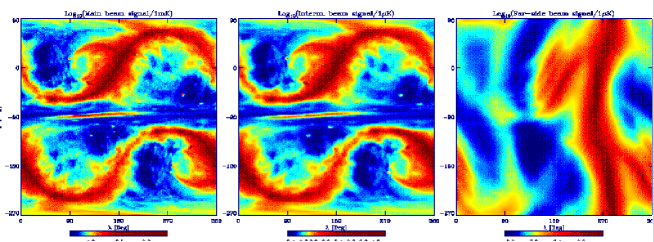
Figure 6: Synthetic view of the data stream from all scans of the Planck-LFI instrument at 30 GHz. The ecliptic coordinates $\lambda$ and $\beta$ are the longitude and latitude of the telescope axis [129].

5.3 Pointing accuracy

The uncertainty in the pointing accuracy may be a serious source of degradation, particularly for high resolution experiments. A typical requirement is a 2$\sigma$ error of 1/10 of the beam FWHM. Experiments from balloon often involve complicated motions both of mirrors (chopping) and of the gondola making pointing repeatibility a non-trivial issue. Satellite instruments experiments are designed to observe the sky with a redundant scanning strategy which involves periodic motion of the satellite as a whole. Therefore the inertia tensor of the satellite has to be known accurately in order to estimate the effects of re-pointing of the satellite on its attitude stability. In order to reduce oscillations induced by pointing maneuvers (both in satellite and balloon-borne experiments) active oscillation damping is sometimes employed.

The uncertainty in pointing direction, as well as the knowledge of such uncertainty, has a direct impact on the effective angular resolution of the experiments, even in the case in which the beam shape is known with high accuracy, and this translates into a restriction of the multipole range effectively probed. The observed signal is a convolution of the sky signal with the beam pattern (see Eq. (34)) together with the statistical distribution of the pointing uncertainty: the net result is a convolution with a beam with a larger FWHM.

Beam shapes from complex optical system are difficult to measure in the laboratory and are usually reconstructed during the observation phase by means of bright point sources such as planets or supernova remnants. The accuracy of beam reconstruction is strongly dependent on the pointing accuracy. Multi-feed experiments require also a “geometrical” calibration of each feed. This means that feed positions with respect to a fiducial reference point have to be determined. We have already seen how off-axis beam patterns differ from a purely circular symmetric Gaussian beam. One could expect to reconstruct the beam shape from point sources and properly account for it. However, pointing accuracy may be a limiting factor for the proper knowledge of beam resolution and beam shape.

In order to solve for the exact pointing solution, one usually has to collect ancillary information. This includes CCD-camera or star-mapper systems to map the sky for bright known stars which requires to know the geometrical configuration of the instrument set-up (focal plane arrangement) and the relative orientation between star-mapper and field of view which can be obtained through observations of bright sources (planets like Jupiter).

5.4 $1/f$-noise instabilities

The presence of $1/f$ noise or of slow drifts in the data stream is a well known problem in CMB experiments. These instabilities typically originate from a combination of thermal fluctuations and amplifier gain variations as well as variatons in the emission of the atmosphere (Sect. 4). For HEMT based microwave radiometers the $1/f$ noise is dominated by gain fluctuations, while for bolometers instabilities may originate in thermal fluctuations of the environment surrounding the detector. The coupling between long-term instabilities and the observing strategy may lead to artifacts in the final map showing up as stripes in the scanning direction. These stripes can increase the overall noise and alter the statistical analysis of the CMB anisotropy.

To first order, $1/f$ noise can be parameterised by a single parameter: the knee-frequency (see Sect. 4.7.1). Of course the knee-frequency depends on different parameters and quantities related to the specific instrument under consideration [130]. A constraint on $f_{\rm k}$ is that it has to be as small as possible compared to the first redundancy frequency $f_{\rm s}$ (linear slew, spin, etc) of the scanning scheme. It is indeed demonstrated [131] that when $f_{\rm k}\,\lower 2.0pt\hbox{${>\atop\hbox{\raise 4.0pt\hbox{$\sim$}}}$}\,f_{\rm s}$ a degradation in the final sensitivity will occur so that the optimal solution would be to design instruments with $f_{\rm k}<f_{\rm s}$. Where this is not possible one is left with the need of removing the artifacts due to $1/f$ noise from the data. If the knee-frequency is well known (and in principle through iterative methods [132] both the noise spectrum and $f_{\rm k}$ can be derived from the data themselves) it is possible to correct the data with a proper noise filter and remove the tail of the $1/f$ noise at low frequencies. In special cases another approach [133, 134] can be applied: it makes no assumption on the noise spectrum and takes advantage of a redundant observing strategy in which repeated observations of the same pixel in the sky can be used. This approach is usually referred to as “destriping”. Even for relatively large values of the knee frequency, the behaviour of $1/f$ noise can be well approximated with a single additive baseline for each redundant data scan. The complete set of intersections between scans is used to solve a linear system where the unknowns are the scan baselines; once the baselines are recovered, they are subtracted from the original scan circle to obtain $1/f$ free data. This approach works remarkably well showing a residual contamination $\,\lower 2.0pt\hbox{${<\atop\hbox{\raise 4.0pt\hbox{$\sim$}}}$}\,4\%$ even for $f_{\rm k}\simeq 7f_{\rm s}$.

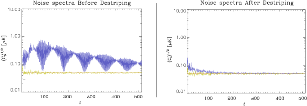
Figure 7: Noise angular power spectra before and after destriping for $f_{\rm k}=0.1$ Hz for a Planck-LFI radiometer at 30 GHz. The noise level after destriping is almost white and comparable with the theoretical white noise level for multipole $\ell\,\lower 2.0pt\hbox{${>\atop\hbox{\raise 4.0pt\hbox{$\sim$}}}$}\,100$ [129].

This is shown in Fig. 7 where the angular power spectrum of a simulated Planck-LFI noise map is plotted before and after applying the destriping technique and compared to the white noise level: a small residual noise is still present at low multipoles, while for $\ell\,\lower 2.0pt\hbox{${>\atop\hbox{\raise 4.0pt\hbox{$\sim$}}}$}\,100$ the noise spectrum is almost indistinguishable from the theoretical white noise spectrum.

5.5 Thermal and periodic fluctuations

Another important class of systematic effects is represented by periodic environment fluctuations (e.g. electrical and/or thermal fluctuations) that may couple with the measured signal and leave spurious signatures in the data. Temperature stability, in particular, is one of the primary concerns that drives many experimental issues, from the instrument thermal design to the observation site and the scanning strategy. Even though a careful choice of the observation site can optimise the ambient thermal stability it is of primary importance that the whole system (active cooling, receivers, and instrument configuration) be properly designed in order to minimise the impact of internally generated thermal fluctuations. The residual effect in the measured data stream can be of the order of few mK peak-to-peak. Therefore it is important to be able to estimate the impact of these spurious signals on the final maps and to further reduce the effect by proper analysis of the time ordered data (TOD).

Under quite general assumptions the peak-to-peak effect of periodic oscillations on the reconstructed sky map can be evaluated analytically [135]. If we consider a periodic fluctuation, $\delta T$, of general shape in the detected signal, we can expand it in Fourier series, i.e.: $\delta T=\sum_{j=-\infty}^{+\infty}A_{j}\exp(i2\pi f_{j}t)$, where $f_{j}$ represents the different frequency components in the fluctuation. For frequencies $f_{j}$ which are not synchronous with the instrument characteristic scanning frequency, $f_{\rm s}$, the measurement redundancy and the projection of the TOD onto a map with a pixel size $\theta_{\rm pix}$ will damp the corresponding harmonic amplitude $A_{j}$ by a factor proportional to $\sin(\pi f_{j}/f_{\rm s})$. For frequencies synchronous with $f_{\rm s}$, instead, there will be no damping and these signals will be practically indistinguishable from the sky measurement. Therefore it is critical that any spurious signal which is synchronous with the characteristic scanning frequency must be carefully controlled and kept at a negligible level in hardware. For a spinning experiment (for example like $MAP$ and Planck ) we can estimate the final peak-to-peak effect of a generic signal fluctuation $\delta T$ on the map as follows:

$$\langle\delta T^{\rm p-p}\rangle_{\rm map} \sim 2\left[\frac{1}{N\times\theta_{\rm pix}/\theta_{\rm rep}}\left(\sum_{f_{j}<k\,f_{\rm s}}\left|\frac{A_{j}}{\sin(\pi f_{j}/f_{\rm s})}\right|+\right.\right.$$

$$+ \left.\left.\sum_{f_{j}<f_{\rm s},f_{j}\neq f_{\rm s}}\left|A_{j}\right|\right)+\sum_{f_{j}=k\,f_{\rm s}}A_{j}\right],$$

where $\theta_{\rm pix}$ is the pixel size, $\theta_{\rm rep}$ is the repointing angle (i.e. the angle between two consecutive scan circles in the sky), $N$ is the number of times each sky pixel is sampled during in each scan circle and $f_{\rm s}$ represents the scan frequency. Note that Eq. (LABEL:eq:p2p_map_general) takes into account the damping provided only by the measurement redundancy and by the scanning strategy, without considering the possibility to detect and partially remove these spurious signals from the TOD. Several numerical strategies can be used to approach this issue and, as a general rule, the removal efficiency is greater with “slow” fluctuations, i.e. with a frequency $f\ll f_{\rm s}$.

An example is shown in Fig. 8 where we plot the damping factor obtained by applying the same destriping algorithm described in section 5.4 to sinusoidal signal fluctuations with various periods; the damping factor is defined as the ratio of the two values of the peak-to-peak effect on the final map obtained before and after application of the destriping algorithm to the data stream. The assumed scanning strategy is representative of a Planck 30 GHz feed-horn. The result clearly shows that the damping factor increases roughly linearly with increasing values of the oscillation period. If we denote with $F_{j}$ the damping factor obtained by applying a certain algorithm to a periodic signal with frequency $\nu_{j}$ then we can write Eq. (LABEL:eq:p2p_map_general) in the more general form:

$$\langle\delta T^{\rm p-p}\rangle_{\rm map} \sim 2\left[\frac{1}{N\times\theta_{\rm pix}/\theta_{\rm rep}}\left(\sum_{f_{j}<k\,f_{\rm s}}\left|\frac{A_{j}/F_{j}}{\sin(\pi f_{j}/f_{\rm s})}\right|+\right.\right.$$

$$+ \left.\left.\sum_{f_{j}<f_{\rm s},f_{j}\neq f_{\rm s}}\left|A_{j}/F_{j}\right|\right)+\sum_{f_{j}=k\,f_{\rm s}}A_{j}\right].$$

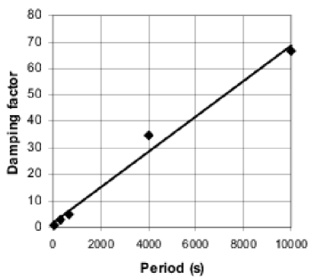
Figure 8: Destriping damping factor for periodic oscillations versus the oscillation period. Dots indicate the values obtained from maps while the solid line represents a linear interpolation.

5.6 Summary

The effects discussed above, as well as the impact of atmospheric and ground radiation (see Sect. 4.4 and 4.5) and calibration (Sect. 4.6), often represent the limiting factors of anisotropy measurements and drive the design of the instrument and data analysis. And the above list is far from complete. Artifacts may be introduced in the data by a number of effects which depend on the intrinsic details of the instrument, such as variable offsets, detectors or amplifiers non-linearities, time-changes of the optics emissivity and of the instrument performance, electrical effects such as ground loops and power instability, magnetic susceptibility, RF interferences. The data processing itself (e.g. data quantisation, data compression, pixelisation, co-adding of multiple scans from different detectors) may be sources of spurious effects. As we shall see in Sect. 7, as the instrument sensitivity improves, the instrument design, scanning strategy and data analysis are more and more focussed on the control and removal of systematics. Sometimes a design choice made to avoid a given effect may itself introduce a secondary source of disturbance. As an example, many sub–degree experiments use a moving (rotating or nutating) subreflector to provide a beam–switching pattern to subtract instrumental and atmospheric drifts (see e.g. [81]). In general, however, strategies that imply moving the subreflector or other reflective parts may raise concern for possible modulation of radiation from the earth (or from the balloon) in the instrument sidelobes.

Each effect is characterised by a set of frequencies and amplitudes, and couples in a peculiar way with the instrument response and the observing strategy. While single effects have been in some cases studied in great detail, of course in the real world they are all hidden simultaneously in the data and may couple with each other in non trivial ways [138]. As we shall see, experiments aiming at few $\mu$K sensitivities, require a proportionally stringent rejection of systematic effects. In addition, precision experiments call for a dedicated effort to understand the impact of the various effects on ancillary measurements such as calibration and beam reconstruction.

6 DATA ANALYSIS

We now present the basic processes involved in the data analysis of CMB anisotropy data which eventually yield the $C_{\ell}$ coefficients and an estimation of the cosmological parameters. The implementation of such processes represents a computation challenge since current experiments produce large amounts of data and much more are expected from the forthcoming satellite missions. The data analysis processes could be regarded as a data (lossless) compression: as an example, for the Boomerang experiments [137] it is possible to pass from the data time stream of few$\times 10^{6}$ elements, to maps with few$\times 10^{4}$ pixels, to power spectrum with coefficients usually binned in few intervals ($\sim 10$) in $\ell$ space.

6.1 Map-making

The first data compression involves passing from the TOD to a map of the surveyed sky area. This map gives a visual impression of what the data look like, and helps in recognising possible systematic effects and astrophysical contamination. In general the problem consists of estimating $N_{p}$ parameters, the signal value in each pixel of the final map, from a large data set of $N_{t}$ observations, producing the best unbiased map. The TOD vector can be written as:

$$\mathbf{d}=A\mathbf{s}+\mathbf{n}\ ,$$ (37)

where $\mathbf{s}$ is the pixelised sky signal, $\mathbf{n}$ is the instrumental noise and $A$ is the pointing matrix with $N_{t}$ rows and $N_{p}$ columns. For a total power scanning experiment, the pointing matrix has the simple form

$$A_{tp}=\bigg{\{}\begin{array}[]{ll}1&{\rm if}(\theta_{t},\phi_{t})\in p\\ 0&{\rm otherwise}\\ \end{array}\,,$$ (38)

where $(\theta_{t},\phi_{t})$ are the coordinates at which the instrument is pointing at the time $t$ falling into the pixel $p$. The best unbiased map is obtained by minimising the quantity:

$$\chi^{2}=(\mathbf{d}^{t}-\mathbf{s}^{t}A^{t})N^{-1}(\mathbf{d}-A\mathbf{s})\ ,$$ (39)

where $N\equiv N_{tt^{\prime}}=\langle n(t)n(t^{\prime})\rangle$ is the noise covariance matrix. Detector noise properties can be derived directly from data either by means of iterative [139] or non-iterative algorithm [140]. The generalised least squares solution gives:

$$\mathbf{\tilde{d}}=(A^{t}N^{-1}A)^{-1}A^{t}N^{-1}\mathbf{d}\ .$$ (40)

Therefore in principle the solution is quite simple: one has to compute the vector $\mathbf{w}=A^{t}N^{-1}\mathbf{d}$ and the matrix $\Sigma^{-1}=(A^{t}N^{-1}A)$ and then invert it to obtain

$$\mathbf{\tilde{d}}=(\Sigma^{-1})^{-1}\mathbf{w}\ .$$ (41)

However, the process involves the inversion of a $N_{p}\times N_{p}$ sparse matrix which requires $\mathcal{O}(N^{3}_{p})$ operations and $\mathcal{O}(N^{2}_{p})$ memory for storage. For $N_{p}$ in the range of $10^{4}\div 10^{5}$ of current experiments, these scalings strongly call for a multi-processor parallel machine. The situation is much more dramatic for future satellite experiments with typical number of pixel around $10^{6}$.

Several algorithms exist for sparse matrix inversion and the case of Conjugate Gradients algorithms is quite interesting [141]. This involves the products of a matrix with a vector, which is an $\mathcal{O}(N_{p}^{2})$ operation. The method is iterative and in general converges in $N_{p}$ iterations unless a good preconditioner $\hat{\Sigma}$ (such that $\hat{\Sigma}\Sigma^{-1}-I\ll 1$) is found. This is usually the diagonal part of the matrix $\Sigma^{-1}$:

$$\hat{\Sigma}={\rm diag}(1/\Sigma_{ii}^{-1})\ .$$ (42)

In this way the algorithm can converge in few tens of operations requiring few minutes for the creation of a $N_{p}=10^{4}$ map on single-CPU workstation. Recently [142] this algorithm has been implemented for the Planck case: processing $N_{t}\sim 3\times 10^{9}$ elements procuding maps with $N_{p}\sim 3\times 10^{6}$ pixels, takes about $10^{3}$ second on 256 processors on an SP3 IBM parallel computer.

6.2 Separating foregrounds from the CMB

As discussed in Sect. 3, a key issue is the separation of foreground emissions from the cosmological signal. This takes advantage of the different frequency and spatial behaviour of the foregrounds with respect to the CMB. Several techniques have been developed for this purpose such as the Wiener filter [143] and Maximum Entropy Method (MEM) [144].

Let us suppose $\mathbf{X}$ is a vector of $M$ observations ($M$ different frequencies) whose probability distribution $P(\mathbf{X}|\mathbf{S})$ depends on the values of $N$ parameters $\mathbf{S}$ (the signal we want to separate). Let $P(\mathbf{S})$ be the prior probability distribution of $\mathbf{S}$ i.e. our a-priori knowledge of the signals $\mathbf{S}$. Given the data $\mathbf{X}$, the Bayes’ theorem states that the posterior probability of $\mathbf{S}$ is given by:

$$P(\mathbf{S}|\mathbf{X})=z\cdot P(\mathbf{X}|\mathbf{S})P(\mathbf{S})\ ,$$ (43)

where $z$ is a normalisation constant. Therefore one has to construct an estimator $\hat{\mathbf{S}}$ of the true signal maximising the posterior probability. The real problem is in the choice of the appropriate prior distribution. Two different approaches have been adopted: the entropic prior and the Gaussian prior.

The entropic prior, which is at the basis of the MEM method, has the form:

$$P(\mathbf{S})\propto{\rm exp}[\alpha H(\mathbf{S,m})]\,$$ (44)

where $\mathbf{m}$ is a model vector to which $\mathbf{S}$ defaults in absence of data, $\alpha$ is a constant depending on the scaling of the problem and $H$ is the cross entropy of $\mathbf{S}$ and $\mathbf{m}$. The MEM method has been applied to CMB map reconstruction [145] assuming the complete knowledge of the frequency scaling of the various components. As for the spatial distribution, two different cases have been considered: the first assumes complete knowledge of the covariance matrix of the signal and in this case the maps are reconstructed with good accuracy; in the second case no assumption is made on the covariance matrix. In this second case reconstruction is obtained only in an iterative way and leads to less accurate results. The CMB power spectrum is in general better recovered than those of the foregrounds.

The Gaussian prior has the form:

$$P(\mathbf{S})\propto{\rm exp}(-\mathbf{S}^{t}\mathbf{C}\mathbf{S})\ ,$$ (45)

where it is assumed that the emission of each component is a Gaussian random field (which is not true in general). Furthermore, a complete knowledge of both the noise ($\mathbf{N}$) and the signal ($\mathbf{C}$) covariance matrices is assumed. This is the Wiener filter which has been applied to data such as DMR [146] and Saskatoon [147].

Recently a new method for foregrounds separation has been proposed [148] based on neural network. This is promising since it does not require any a-priori knowledge of either frequency scaling or spatial distribution of the components to be separated. The only requirement is that at most one of the signal has to be Gaussian (the CMB) and that the signals are statistically independent. Preliminary results without instrumental noise are encouraging, yielding output maps exactly reproducing the input ones, a part from a scaling constant. On the same line, a recent work [149] implements a fast Independent Component Analysis (ICA) technique applied to simulated Planck observations. This approach takes into account the instrumental noise, although it is assumed to be white and uniformly distributed on the sky. Results are extremely good: the CMB angular power spectrum is recovered to high precision (up to $\ell\simeq 2000$) with the correct signal normalisation, as well as the expected CMB frequency scaling. The algorithm is extremely fast (few minutes to separate components for map with $\sim 10^{6}$ pixels). One of the main limitations is that the algorithm it not able, in the present version, to perform simultaneously beam deconvolution. This implies that input maps have to be at the same angular resolution.

In recent years it has become clear that “blind” algorithms, such as those exploiting ICA techniques, represent an optimal tool to derive “priors” on the components to be separated, making such assumptions less sensitive to our incomplete knowledge of astrophysical signals. These “priors” can then be fed into more sophisticated algorithms, like MEM, for a full complete analysis, inlcuding deconvolution.

6.3 Power spectrum estimation

Once we have compressed the TOD into a map and cleaned it from astrophysical foregrounds and possible systematic effects, we have to extract from it the cosmological information mostly embedded in the $C_{\ell}$ coefficients. The problem of deriving the $C_{\ell}$’s scales as $\mathcal{O}(N_{p}^{3})$ and at present no general solution is available.

The problem is quite simple in principle. The set of $C_{\ell}$, convolved with the window function $W_{\ell}$, are obtained maximising the likelihood function:

$$\mathcal{L}(C_{\ell}|\mathbf{\tilde{d}})=\frac{{\rm exp}\left(-\frac{1}{2}\mathbf{\tilde{d}}^{t}\mathbf{C}^{-1}\mathbf{\tilde{d}}\right)}{(2\pi)^{N_{p}/2}({\rm det}\mathbf{C})^{1/2}}\ ,$$ (46)

where $\mathbf{C}$ is the map covariance matrix (signal plus noise). The most likely power spectrum is found expanding the log-likelihood function in Taylor series about the minimum. After some computation the solution, found iteratively, is:

$$C_{\ell}^{n+1}=C_{\ell}^{n}-\frac{1}{2}\sum_{\ell^{\prime}}\mathbf{F}_{\ell\ell^{\prime}}^{-1}\frac{\partial f}{\partial C_{\ell^{\prime}}}\bigg{|}_{C_{\ell^{\prime}}^{n}}\ ,$$ (47)

where $f=-2{\rm ln}\mathcal{L}$ and $\mathbf{F}_{\ell\ell^{\prime}}$ is the Fisher information matrix:

$$\mathbf{F}_{\ell\ell^{\prime}}=-\bigg{\langle}\frac{\partial^{2}}{\partial C_{\ell}\partial C_{\ell^{\prime}}}{\rm ln}\mathcal{L}\bigg{\rangle}\,.$$ (48)

The system can be solved using the Newton-Raphson method which usually converges in 3-4 iterations but the convergence is quadratic only in a neighborhood of the root. Furthermore, as stated above, the matrix inversion takes $\mathcal{O}(N_{p}^{3})$ operations, but in this case it is not easy to find a good preconditioner as for the map-making problem. This is because the $\mathbf{C}$ matrix depends both on noise and signal which essentially belong to different spaces. While the noise covariance matrix is diagonal in pixel space it is dense in $Y_{\ell m}$ space and the reverse is true for the signal covariance matrix. So a general solution is not at hand. Furthermore any basis transformation that would make $\mathbf{S}$ and $\mathbf{N}$ diagonal or block-diagonal cost $\mathcal{O}(N_{p}^{3})$ operations and it is of no use. A good preconditioner has been found by the $MAP$ team [150] since the $MAP$ scanning strategy generates noise patterns which are nearly azimuthally symmetric. However this is not true for balloon experiment and has to be carefully investigated for Planck. It is worth noting that the only case for which the maximum likelihood problem has been solved exactly, is $COBE$-DMR, for which the $\mathcal{O}(N_{p}^{3})$ scaling was still treatable [151, 152, 153].

A code called MADCAP has been developed [154] and has been used to compute the maximum likelihood power spectrum for the Boomerang [137] and Maxima [155] experiments. This works on a Cray-T3E parallel machine and allows the computation of the power spectrum in a reasonable time for a suitable number ($\approx$ 10) of bins in $\ell$ space in the range 30-800. However, current experiments require a solution able to handle much larger data sets. Among the new proposed approaches that dramatically reduce the number of operations, we mention the Ring-Torus method [156] and the MASTER technique [157]. The first is extremely elegant in its algebraic properties and works quite well for a limited set of observing strategies, including those of $MAP$, as well as for Planck, if the spin-axis is kept always on the ecliptic plane (see Sect. 8.3.2). In these cases exact maximum likelihood power spectrum (Eq. (46)) is possible with $\mathcal{O}(N_{p}^{2})$ operation since both signal and noise matrices are block-diagonal in Fourier space.

The MASTER method is based on a direct spherical harmonic transformation of the cleaned CMB map and allows to include specific features of the observation (e.g. survey geometry, scanning strategy, noise properties) together with possible non-Gaussian and non-stationary processes that can occur during the experiment life time. The resulting power spectrum is corrected for characteristics of the instrument and observing strategy as well as any operation performed in the data analysis process, by means of Monte Carlo simulations. The final power spectrum has been demonstrated to be an unbiased estimator of the true CMB power spectrum. This technique was applied to the Boomerang data [158] covering 1.8% of the sky (57,000 pixels with $7^{\prime}$ resolution). It is proved to be extremely fast and easily parallelisable and can be considered as a valuable tool for more extensive applications. Recently applications of the MASTER approach have been implemented using general least squared map-making algorithm [159] yielding similar results of the original MASTER method.

Other approaches to the problem involve computation of the 2-pt correlation function of the sky and then invert it to obtain the angular power spectrum [160]. On the same line similar results have been obtained computing the 2-pt correlation function of the CMB peak distribution [161].

6.4 Extracting cosmological parameters

Once we have the CMB angular power spectrum, it is possible to apply the usual likelihood approach to derive the cosmological parameters $\mathbf{p}=(\Omega_{b},\Omega_{\rm CDM},\Lambda,H_{0},n_{S},n_{t},...)$. Proceeding in a similar way as for the power spectrum estimation, the Fisher information matrix for cosmological parameters is given by:

$$\mathbf{F}_{kk^{\prime}} = -\bigg{\langle}\frac{\partial^{2}}{\partial p_{k}\partial p_{k^{\prime}}}{\rm ln}\mathcal{L}\bigg{\rangle}$$

$$= -\sum_{\ell\ell^{\prime}}\frac{\partial C_{\ell}}{\partial p_{k}}\bigg{\langle}\frac{\partial^{2}}{\partial C_{\ell}\partial C_{\ell^{\prime}}}{\rm ln}\mathcal{L}\bigg{\rangle}\frac{\partial C_{\ell^{\prime}}}{\partial p_{k^{\prime}}}$$

$$= \sum_{\ell\ell^{\prime}}\frac{\partial C_{\ell}}{\partial p_{k}}\mathbf{F}_{\ell\ell^{\prime}}\frac{\partial C_{\ell^{\prime}}}{\partial p_{k^{\prime}}}$$

The partial derivatives with respect to cosmological parameters can be computed numerically using two-side finite differences of order 2-5% of the parameter value using model spectra computed with fast numerical codes [52]. However, in this case it is not so easy to exploit the Newton-Raphson method since the radius of convergence is quite smaller and, in addition, the degeneracy between various parameters creates features in the likelihood which makes the Newton approach not optimal. One can instead proceed with a simple $\chi^{2}$ fit:

$$\chi^{2}(\mathbf{p})=\sum_{\ell\ell^{\prime}}(C_{\ell}(\mathbf{p})-C_{\ell}^{\rm recov})\mathbf{F}_{\ell\ell^{\prime}}(C_{\ell^{\prime}}(\mathbf{p})-C_{\ell^{\prime}}^{\rm recov})\ ,$$ (50)

where $C_{\ell}(\mathbf{p})$ is the theoretically computed power spectrum and $C_{\ell}^{\rm recov}$ is the recovered one. This method has been tested by the $MAP$ team [150] yielding excellent results in the multipole range where the signal-to-noise ratio is high enough ($\ell\,\lower 2.0pt\hbox{${<\atop\hbox{\raise 4.0pt\hbox{$\sim$}}}$}\,600$).

It is clear that the final accuracy depends also on the accuracy by which theoretical models are computed. Present fast algorithms that integrate the Boltzmann equation to find the CMB angular power spectrum, provide accuracy at the percent level, i.e. compatible with the Planck goal accuracy on the parameter estimation. It is clearly of great interest to develop codes that would be equally, or even more, fast but with improved accuracy.

7 ANISOTROPY EXPERIMENTS

In this section we review the CMB anisotropy experiments carried out from $COBE$-DMR up to now. Some of the key features of all experiments leading to anisotropy detection are summarised in Table I-IV. We first outline the DMR experiment, and then we review ground-based and balloon-borne experiments. Finally we provide a synthesis of the current status of power spectrum measurements.

7.1 The $COBE$ Differential Microwave Radiometer

On 18 November 1989, NASA’s $COBE$ satellite (see Fig. 9) was launched from Vandenberg Air Force Base into a near-polar circular orbit. It was the starting point of one of the greatest achievements in the history of CMB experiments, and indeed of cosmology at large: the first unambiguous detection of structure in the CMB angular distribution. The first detection was obtained on angular scales $>7^{\circ}$ by the Differential Microwave Radiometer (DMR) based on its first year of data [15, 162]. These early results were supported by detailed calibration [92] and systematic errors analysis [86]. The first detection was soon confirmed by the positive cross-correlation between $COBE$-DMR and sub-orbital observations [163, 164]. Later, the results from DMR’s first two years observations [87] were shown to be consistent with those from the first year alone. The DMR mission ended in December 1993, after 4 years of uninterrupted survey. The definitive DMR analysis and results are reported in [165, 166, 167, 168, 169, 170, 89, 171, 172, 173].

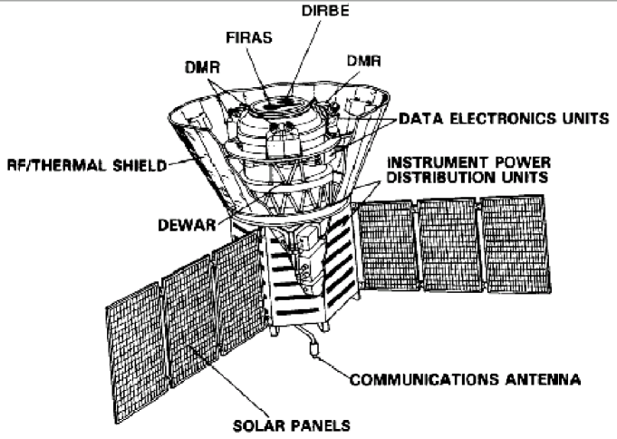
Figure 9: The Cosmic Background Explorer ($COBE$) satellite showing the Differential Microwave Radiometers (DMRs), Data Electronics Units, and Instrument Power Distribution Units as mounted on the $COBE$ spacecraft. The spacecraft spins about its axis of symmetry. (From [94] with permission.)

The instrument [94] consisted of six Dicke-switched differential radiometers, two independent systems at each observing band centred at 31.5, 53 and 90 GHz. Each radiometer measured the difference in power received from two directions in the sky separated by 60^∘, using a pair of corrugated horn antennas at symmetric angles with the spin axis. The antenna beams were highly symmetric with FWHM $\simeq 7^{\circ}$. The receivers were superheterodyne systems switched at 100 Hz, using a single local oscillator per frequency assembly.

The $COBE$ satellite spun at approximately 0.8 rpm and precessed in a 900 km near-polar orbit, following the day-night terminator. This allowed the instrument to always point away from the earth and be perpendicular to the sun, thus minimising straylight effects. The combination of the satellite spin (75 s), orbit (103 min), and orbital precession ($\sim 1$ degree/day) provided a redundant set of temperature differences spaced $60^{\circ}$ apart, and allowed to cover the entire sky in a six-month period. Systematic thermal and electrical modulations occurred near the summer solstice, for about 60 days per year, since the earth was not fully screened by the satellite shields as the spacecraft approached the North Pole, while at the South Pole eclipses occurred every orbit.

In-flight relative calibration was provided by solid state noise sources injecting broad band power in the radiometers front end every 2 hours. The moon signal provided further check to the calibration, with an accuracy limited by the uncertainty in the model of the moon antenna temperature and phases. The most accurate absolute calibration was derived from the 30 km s^-1 earth’s motion around the solar system baricentre, which produces a $\sim 0.3$ mK Doppler shift dipole of accurately known amplitude (see Sect. 4.6).

The careful analysis of potential and detected systematic effects [86, 89] included emission from earth and the moon, the instrument’s response to thermal instabilities, and the effect of earth’s magnetic field. The analysis showed that even the largest detected effects did not contribute significantly to the DMR maps. Data taken in worst-case situations for potential straylight contamination and from thermal fluctuations were rejected ($\lesssim 10\%$ of the data), while the remaining data were corrected using models of each effect. The estimated upper limit to residual systematic artifacts in the maps was $<6~{}\mu$K (95% C.L.), i.e. significantly less than the noise levels of sky signals.

With the full 4-year data, the typical signal-to-noise ratio of the frequency-averaged map smoothed at $10^{\circ}$ was $\sim 2$, which means that the final DMR CMB map does provide a visual impression of the CMB structure in the sky. Monopole ($T_{0}=2.725\pm 0.020$ K) and dipole ($\Delta T_{\rm dip}=3.353\pm 0.024$ mK) measurements from DMR were reported in [89, 8]. The intrinsic quadrupole ($\ell=2$) amplitude was found to be $\Delta T_{2}=10.0^{+3.8}_{-2.8}~{}\mu$K (68% confidence level). The value predicted by a power-law fit to the power spectrum yielded $Q_{rms-PS}=15.3~{}\mu$K [170, 168]. The observed power spectrum at large angular scales, which was limited by cosmic variance for $\ell<20$, was found to be consistent with a $n_{S}\simeq 1$ power law [166, 168, 169]. Assuming $n_{S}=1$, then the best-fit normalisation was found to be $Q_{{\rm rms-PS};n=1}=18\pm 1.6$ $\mu$K. Finally, the combined 31, 53, and 90 GHz map smoothed at $10^{\circ}$ yielded a CMB rms of $29\pm 1$ $\mu$K. The DMR full-sky map allowed also testing for the Gaussianity of the temperature distribution [89], which was found to be consistent with Gaussian statistics.

These results set the stage for new major efforts: anisotropies were now known to exist at amplitudes $\Delta T/T\sim$ $10^{-5}$, and the race to unveil new features in the angular power spectrum (especially with sub-degree scale observations) was started.

7.2 Ground-based

High altitude, dry ground based sites have provided remarkable CMB anisotropy results, in spite of the limitations of atmosphere and ground emissions, although in small sky patches. Even if harsh and isolated, ground based operations offer the enormous advantage of reachable instruments and long integration times. The Python experiment, which operated at the South Pole during the 1996-1997 austral summer, found that the atmosphere could rarely be seen in the data; the experiment was noise limited 75% of the time [175]. DASI data suggest that during the austral winter, the efficiency is closer to 90%. The Polar environment during Antarctic winter is probably the most favorable condition for a CMB ground based experiment. In addition, the South Pole provides access to a region of sky with some of the lowest dust column densities, as inferred from the IRAS 100-$\mu$m map of the southern sky.

7.2.1 UCSB South Pole

Among the first experiments to systematically probe the sub-degree portion of the power spectrum, this was a program by the University of California at Santa Barbara which led to a series of three measurement campaigns from the Amundsen-Scott South Pole Station in the period 1988-1994. All of these experiments were carried out with HEMT-based coherent receivers, cooled at cryogenic ($T_{\rm phys}\simeq$ 4 K) temperatures. The observing frequencies were in the atmospheric window around 30-40 GHz (Ka and Q bands). The results from the 1988-1989 measurements are described in [83] and [84] while the results from the 1990-1991 measurements are detailed in [176] and [177].

The third campaign, during the austral summer 1993-1994, provided the most accurate results of this effort [178]. Each observation employed a 3 degree peak-to-peak sinusoidal, single difference chop scanning strategy. The observed sky was a $20^{\circ}\times 1^{\circ}$ strip. Two sets of observations were performed: the first used a receiver operating in three channels between 38 and 45 GHz (Q-band) with FWHM varying from 1^∘ to 1.15^∘; the second overlapped the first one, and used a receiver operating in four channels between 26 and 36 GHz with FWHM varying from 1.5^∘ to 1.7^∘. Significant correlated structure was observed in all channels for both observations leading to an amplitude $\delta T_{\ell}\sim$ 30-35 $\mu$K at $\ell\simeq 60$. The spectrum of the detected structure was proven to be compatible with CMB, while a spectral analysis showed inconsistency (at $5\sigma$ level) with a diffuse synchrotron or free-free emission. In addition, the amplitude of the observed fluctuations was inconsistent with 20 K interstellar dust; however, the data were not able to discriminate against contamination from flat or inverted spectrum point sources.

7.2.2 WD

The “White Dish” experiment [179, 180] carried out by a U.S. collaboration, was a ground-based bolometer detector centred at 90 GHz, cooled at 100 mK by an adiabatic demagnetisation cooler. The bolometer with 30% bandpass had a sensitivity $\sim 5$ mK$\times$Hz^-1/2. The instrument used an on-axis Cassegrein telescope, with the secondary reflector slightly displaced from the optical axis of the main reflector, yielding a beam size of $12^{\prime}$ [181, 179]. The structure supporting the subreflector was designed to minimise diffraction effects, and two radiation shields surrounded the telescope during the observations. Deep side-lobes measurements were performed showing a rejection $<-85$ dB at angles greater than $50^{\circ}$.

The observations were made from the Amundsen-Scott South Pole site in January 1993. Five interlocking circles in the sky were scanned, with centres separated by $15^{\prime}$ at constant elevation angle, minimising spurious effects from the atmosphere, from the ground as well as gravitational effects on the instrument. Calibration was performed at the beginning and at the end of the each 6-hour measurement run by placing warm absorber on the main reflector and filling the beam with blackbody targets cooled with liquid N₂ and O₂, yielding a calibration uncertainty of $\sim 30\%$. A total of 150 hours data were collected, about 14% of which were used in the final analysis. No conclusive evidence of anisotropy detection was obtained, but an upper limit was found, $\Delta T/T<2.3\times 10^{-5}$ at 95% confidence level, corresponding to $\Delta T_{\ell}<$35 $\mu$K at $\ell\sim 60$.

7.2.3 IAC-Bartol

In the summer of 1994, a collaboration between the groups from IAC and Bartol carried out observations from the Tenerife site at angular scales $\sim 2^{\circ}$ [182]. Together with Python and SuZIE, this was one of the few ground-based experiments at frequencies $>100$ GHz: four bands were used centred at 91, 142, 230, and 273 GHz. The instrument was based on bolometric detectors in a 4-channel photometer cooled at approximately 0.33 K with ³He [183, 184]. An off-axis Gregorian telescope was employed, with a 45-cm primary reflector and a 28-cm secondary, leading to approximately equal beams with FWHM$=2.03^{\circ}\pm 0.09^{\circ}$ at the four observing frequencies. The primary reflector was sinusoidally wobbled, thus moving the beam in the sky by about $\pm 2.6^{\circ}$ at 4 Hz. The signal was then demodulated in software by evaluating the first and second harmonics of the wobble frequency. Calibration was performed with blackbody targets in the laboratory and against the moon signal, leading to uncertainties at 5% – 25% level, depending on frequency. The drift-scan observations were centred at $\delta=40^{\circ}$, a region of the sky intensively observed at 10-33 GHz by the Jodrell Bank - IAC experiment [185, 186], though at larger $\sim 5^{\circ}$ scales (see Sect. 7.2.4).

The main challenge was to disentangle the high atmospheric contribution due to O₂, H₂O and O₃ emission lines at millimetric wavelengths. The strong atmospheric signal showed up as a correlated time-variable signature, which was removed by relying on the 273 GHz channel as a monitor. Foreground Galactic emission was excluded to significantly contribute based on extrapolation of templates of Galactic emission and using external data. The data demodulated at the two harmonics showed some inconsistency which was attributed to residual atmospheric effects. A two-component likelihood analysis gave an estimate of the CMB fluctuation $\Delta T_{\ell}=4.1^{+2.4}_{-2.2}\times 10^{-5}$ $\mu$K in the bandpower $\ell=33^{+24}_{-13}$ and $\Delta T_{\ell}=2.0^{+1.0}_{-0.8}\times 10^{-5}$ $\mu$K in $\ell=53^{+22}_{-15}$.

Recently a third campaign has been carried out with an improved angular resolution of 1.35^∘ at all wavelengths [187]. These measurements provided anisotropy detection in the multipole range $39<\ell<134$. While this experiment showed that it is possible to detect CMB anisotropy with ground-based measurements at high frequency, it also clearly showed the very significant limitation imposed by the atmospheric signal in this regime.

7.2.4 Tenerife

The Tenerife experiment employed three radiometers centred at 10.4, 14.9 and 33 GHz, designed and built at Jodrell Bank ([188], [189], [81], [58]), and operated in collaboration with the Instituto de Astrofisica de Canarias (IAC) group in Tenerife. Each instrument (see Fig. 10) consisted of dual-beam radiometer, with a pair of horns maintained fixed in the horizontal direction, coupled to a tilted wagging secondary flat reflector with a beamthrow of 8.1^∘. This resulted in a synthetic triple beam pattern in the sky, which helped considerably in removing receiver long-term fluctuations as well as the effect of atmospheric emission. At each frequency, two independent Dicke-switched receivers cooled at $\sim$70 K with liquid N₂ were used, thus improving sensitivity by a factor of $\sqrt{2}$. The measurements were sensitive to angular scales of $\sim 5^{\circ}$, or $\ell\sim$ 10-30, which correspond to the Sachs-Wolfe plateau.

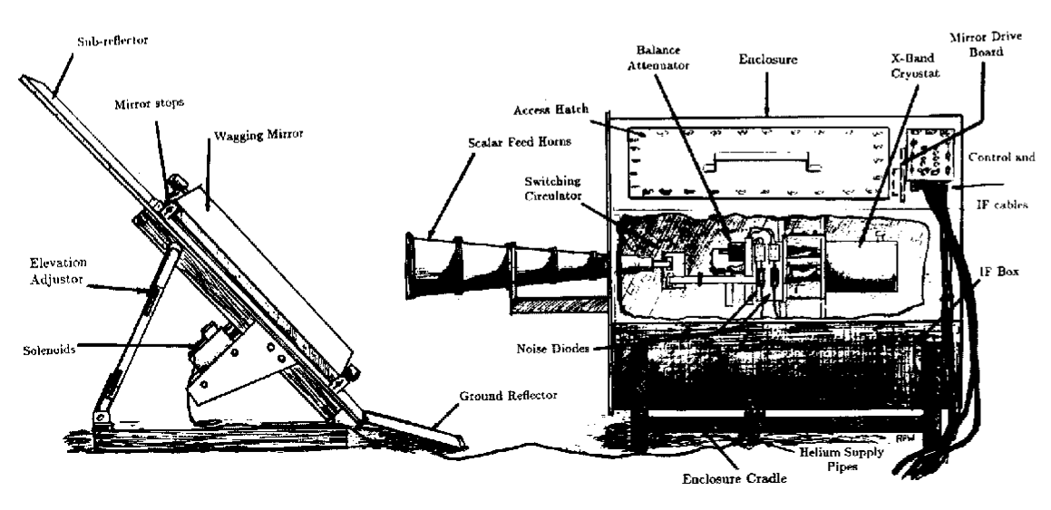
Figure 10: A sketch of the arrangement of the 10.45 GHz beam switching system. A weatherproof enclosure houses the horn support, the switching circulator and the cryogenically cooled receiver system. The IF bands from the two independent receiver systems are fed to a building 30 m distant, where they are detected and recorded. The wagging mirror is operated by two solenoids in a 14-s cycle; a guard mirror surrounds it. Declination can be set by altering the mirror elevation. (From [81] with permission.)

The observations were carried out at the Teide Observatory, Izana, at an altitude of 2400 m. The good observing site (stable atmospheric emission and typical water vapour content 2–3 mm [190]) and the advantageous observing strategy, helped reducing data loss. Nonetheless, at 33 GHz, where the H₂O contribution is highest, only about 20% of the time was usable.

The data were taken by drift scans in right ascension and at a fixed declination. By sampling at $2.5^{\circ}$ intervals in declination with a $5.1^{\circ}$ FWHM, fully sampled two-dimensional maps were constructed at each frequency [191]. A first set of observations scanned a sky strip at declination $+40.0^{\circ}$ (a relatively low foreground region) while subsequent observations covered adjacent sky strips, between declination $+30^{\circ}$ and $+45^{\circ}$.

As discussed in Sect. 3, in the 10-40 GHz range the dominant foreground emission comes from diffuse Galactic synchrotron and free-free emission. Between 10 and 33 GHz the free-free component scales by a factor of $\sim 10$, while synchrotron emission scales by as much as a factor $\sim 25$. Thus the combination of the three instruments provided a good spectral leverage, and in particular the 10.4 GHz channel was used in the analysis to check against contamination from these foregrounds.

The first clear detection of CMB structure by the Tenerife collaboration [185] showed evidence of cosmic anisotropy at a level $\sim 40$ $\mu$K. The Tenerife observations provided the first ground-based detection of CMB anisotropy, following the space-born DMR [15] and the balloon-borne FIRS data [96]. It should also be mentioned that the results from this experiment were the first in which the signal to noise ratio per resolution element was sufficiently high to actually “image” stable hot and cold spots in the CMB pattern. The most recent analysis of the Tenerife effort [192] covered observations over 5000 and 6500 square degrees at 10 and 15 GHz respectively, centred around declination $+35^{\circ}$. The ultimate receiver noise per resolution element was 31 and 12 $\mu$K at 10 and 15 GHz respectively. The data showed clear detection of structure at high Galactic latitude. Including upper limits to possible galactic contamination effects, the measured CMB signal was $\Delta T=30^{+15}_{-11}$ $\mu$K. These values were highly stable against the Galactic cut chosen and were found to be compatible with the $COBE$ DMR data.

7.2.5 Python

Five observing campaigns from the South Pole Station were performed by the Python experiment, lead by the group at Carnegie Mellon University at Pittsburgh, each leading to detection of CMB anisotropy at $\sim 1^{\circ}$ scales. The set up consisted of a 0.75 m diameter off-axis parabolic telescope coupled either to a bolometer system at 90 GHz or to a HEMT amplifier-based radiometer at 40 GHz.

Observations from the first three seasons [193, 194, 195] were made at 90 GHz with an array of 4 corrugated horns feeding germanium bolometers cooled to 50 mK by a ³He adiabatic demagnetisation refrigerator [196]. The four-point chop scan strategy yielded CMB detections at $\ell\simeq 90$ and $\ell\simeq 170$. The beam was well approximated by a Gaussian with FWHM $\sim 0.75^{\circ}$. Radiation from the sky was first reflected by a chopping (100 Hz) flat reflector, and then focussed into the cryostat by the primary mirror. Single-mode waveguide filters were used to define the band. An additional “blind” bolometer was mounted on the cold stage as a monitor against systematic effects. In addition, the overlap in the regions observed in the three campaigns was exploited for diagnostics including effects from atmospheric emission, pointing and beam calibration, cosmic ray hits in the detectors, radio-frequency interference, and sun radiation. The instrument calibration was based on a combination of warm and cold targets and the moon, leading to an accuracy of $\pm\sim$10% limited by systematic effects. The lack of spectral information prevented direct discrimination of galactic foregrounds, although analysis from external surveys [197] indicated that galactic contamination was likely to be small.

In the fourth and fifth Python campaigns [198], [199], the telescope was equipped with a HEMT amplifier radiometer, covering the 37-45 GHz range with a beam of about 1^∘. The receiver consisted of two focal-plane feeds, each with a single HEMT amplifier and a diplexer splitting the signal at 41 GHz before detection, thus giving four data channels [198]. Calibration was performed with liquid nitrogen, liquid oxygen and ambient temperature external targets, leading to $<15\%$ accuracy. In the most recent campaign [199] two regions were observed, sampling 598 square degrees in the sky: the first included the fields of the previous four Python observations, the second encompassed the region observed with the Advanced Cosmic Microwave Explorer (ACME) telescope [200]. To search for potential foreground contamination the data were cross-correlated with several foreground templates [201, 202] (Parkes-MIT-NRAO 4.8 GHz radio survey, PMN), and significant contamination from known foregrounds was excluded.

The power spectrum results from Python were consistent with $COBE$-DMR at low $\ell$, and indicated an increase at multipoles $40<\ell<260$ from larger to smaller angular scales.

7.2.6 Viper

The Viper experiment, also led by the group at Carnegie Mellon University at Pittsburg, was conceived as a follow up of Python at higher angular resolution. The first results were obtained with observations from the South Pole [203] at 40 GHz. At this frequency the Viper 2.15 m telescope yielded a 16 arcmin FWHM main beam, with an angular sensitivity in the range $100<\ell<600$.

The rather sophisticated optics consisted of an aplanatic Gregorian with the addition of a flat, electrically driven chopping mirror (oscillating at 2.35 Hz), and of a fast hyperbolic mirror redirecting the radiation to the radiometer [204]. Extensive shielding around the primary and a 10-m baffle surrounding the whole instrument were employed to minimise ground radiation pickup. The radiometer was a two-channel receiver based on HEMT cryogenic ($\sim$20 K) amplifiers, coupled to the telescope through corrugated feed horns. The instrument measured the total power from 38 to 44 GHz, in two sub-bands, and was calibrated using targets at ambient and liquid-nitrogen temperatures with an estimated accuracy of $8\%$. The main beam pattern ($0.26^{\circ}\pm 0.01^{\circ}$) and chopper throw ($3.60^{\circ}\pm 0.01^{\circ}$) were calibrated using observations of Venus.

Particular care was taken to remove offsets synchronous with the chopping mirror modulation, e.g. due to synchronous changes of illumination of the secondary mirror or to scattering by snow grains on the optics.

The estimate of galactic foregrounds was based on the overlap with the sky region observed by Python. Using IRAS data [205] and the Parkes-MIT-NRAO survey data, an upper limit $<1$ $\mu$K was estimated from dust, synchrotron or free-free emission [199]. Due to the higher angular resolution extra-galactic point sources were a more serious concern compared to Python. Using PMN 4.8 GHz data the effect from the brightest known point source (PMNJ2256-5158) was subtracted at a level of $<2$ $\mu$K. Extrapolation of IRAS 100 $\mu$m sources near the observed region lead to sub-$\mu$K limits. In this and similar measurements, however, there remains the possibility of contamination from a class of undetected objects with spectra that closely mimic the CMB, such as dusty galaxies at high $z$. High angular resolution sky surveys would be needed to rule out this potential source of confusion. Interpreting the power observed as due to CMB anisotropy, the results yielded $\Delta T_{\ell}\approx 60$ $\mu$K, with a hint of the presence of the first peak near $\ell\approx 200$.

After these measurements the Viper telescope was used to carry out a survey of a complete sample of 14 luminous X-ray clusters at $z<0.1$ [206], with the aim of measuring the Sunyaev-Zel’dovich signal in the 45 - 350 GHz range.

7.2.7 Saskatoon

This ground-based program, carried out by the Princeton group, probed angular scales between 0.5^∘ and 3^∘, or multipoles $60<\ell<360$, and produced one of the first convincing evidences for the presence of the first peak in the power spectrum. The observations were made in the winters of 1993, 1994 and 1995 from a site in Saskatoon, Saskatchewan, Canada. The instrument [207, 208] used an off-axis parabolic reflector coupled to cryogenically cooled total power receivers based on low-noise HEMT amplifiers. After the parabola, the beam was directed in a flat reflector chopping in azimuth at 3.9 Hz, while the radiometer channels were synchronously sampled at 250 Hz. Extended aluminum shields were built around the instrument. The observations were made by two independent radiometers, alternating each other at the focus of the same telescope: one operated in the Ka-Band (26-36 GHz) and another in the Q-Band (36-46 GHz). Each of these bands were divided into 3 frequency “sub-bands” and 2 polarisations. The beam FWHM of the Ka-Band and of the Q-Band were 1.42^∘ and 1.04^∘ degrees, respectively. To improve the sensitivity to multiple angular scales, the beam was scanned back and forth about the vertical axis, giving an effective beam pattern that was synthesised in software. This technique also helped to remove atmospheric noise and allowed to suppress the effect of ground and solar radiation. For calibration and beam shape measurements, Cassiopea-A was used as a source.

As mentioned, the Saskatoon data provided evidence for a raising spectrum, going from $T_{\ell}=49^{+8}_{-5}$ $\mu$K at $\ell=87$, to $T_{\ell}=85^{+10}_{-8}$ $\mu$K at $\ell=237$. The 1993-1995 data were also used to construct a Wiener-filtered map [147] in a $15^{\circ}$ cap centred in the NCP, with an angular resolution of $\sim 1^{\circ}$. The signal-to-noise ratio in the map was of order 2. Some individual hot and cold spots were significant at the 5 $\sigma$ level and were found to be consistent for different observations. The spectral coverage of the Saskatoon experiment was too low for a self-consistent removal of foregrounds, so external information was used. No significant correlation was found with point sources, with the Haslam 408 MHz map, or with the Reich and Reich 1420 MHz map. However, some correlation was found with the DIRBE 240, 140 and 100 $\mu$m maps, with an rms amplitude of the correlated component $\sim 20\%$ of the CMB signal [209].

7.2.8 MAT/TOCO

As a continuation of the Saskatoon and QMAP experiments (see Sect. 7.2.7 and 7.3.6), the MAT (Mobile Anisotropy Telescope) collaboration was established between Princeton University and University of Pennsylvania to extend the program of sub-degree measurements. The instrument used the telescope successfully employed in two QMAP balloon flights in 1996. The MAT instrument, sensitive to angular scales from $\ell\simeq 40$ to $\ell\simeq 600$ had angular resolution and frequency coverage chosen to overlap and complement the $MAP$ data (see Sect. 8.3.1). In addition to channels at 31 and 42 GHz, overlapping $MAP$, MAT had a 144 GHz channel with a 0.2^∘ degree beam. At this angular scale $MAP$ observes at 90 GHz. The 144 GHz channels are relatively immune from extra-galactic sources and galactic foreground emission, and will be useful to constrain potential contamination in $MAP$.

The receiver took advantage of both HEMT and SIS technologies, both cooled with a mechanical refrigerator. Two Ka-band HEMT channels (26-36 GHz) observed the same pixel on the sky in two orthogonal polarisations, and four Q-band HEMT channels (36-46 GHz) observed two orthogonal polarisations at each of two independent pixels. The front-end HEMTs were cooled at 36 K while the SIS mixers were operated at 4 K. An off-axis 85 cm paraboloid was illuminated by the focal array of corrugated feeds with an edge taper of about -25 dB, providing beam widths $\sim$0.7^∘ at Ka-Q bands and $\sim$0.2^∘ in D band. A large chopping flat reflector (1.8 m) was used to sweep the beam across the sky, with a scanning strategy similar to that of Saskatoon [208].

The observations were carried out from Cerro Toco in northern Chile from a site at an altitude of 5240 m with excellent atmospheric characteristics. Two analyses have been published covering the 1997 data at 30-40 GHz [210] and the 1998 data at 144 GHz [112]. The observations in the two campaigns concentrated on the same sky region, and the analysis indicated that the detected structure is fully compatible with the CMB spectral distribution. The results suggested that the angular spectrum peaks at approximately 85 $\mu$K at $\ell\sim$200, consistent with a $\Omega_{0}\approx 1$ scenario.

Detailed design features and analysis of systematic effects was described in [211], including microphonics, earth emission, atmospheric noise. Systematic residual offsets at 2-8 mK level were observed. TOCO was calibrated using Jupiter [212, 213] providing a signal level in the range 15–350 mK, with an intrinsic calibration error of 5%.

A quantitative analysis of foregrounds was carried out using the SFD dust map [70], the Haslam map [202], and the radio and IRAS source compilations from WOMBAT. The dominant source in the Ka and Q bands was from the radio point sources as traced by the 4.85 GHz PMN catalog [214, 215, 216]. No significant contamination from either dust or point sources was found at 144 GHz.

Recently [211] a detailed analysis of the combined QMAP and MAT/TOCO experiments was published. The MAT/TOCO experiment provided a self-consistent data set with evidence of both the rise and the fall of the first peak, with an estimated position $\ell_{peak}=216\pm 14$.

7.2.9 CAT

The Cosmic Anisotropy Telescope interferometer was developed by the Cambridge group, and carried out observations from a site near Cambridge. It is a three-element array that can operate at any frequency between 13 and 17 GHz. The system has an observing bandwidth of 500 MHz, a system temperature of $\sim 50$ K and it simultaneously records data from orthogonal linear polarisations. The baselines can be varied from 1 to 5 m, and for CMB observations a synthesised beam of approximately 0.5^∘ is used. The three antennas have a diameter of 70 cm and the primary beam has a FWHM of 2^∘ at 15 GHz, and they are mounted on a single turntable which can track in azimuth. To reduce the effect of spill-over and artificial radio interference, the telescope is surrounded by a 5-m high ground shield which, on the other hand, limits observations to elevations $>30^{\circ}$.

The first set of CAT multifrequency observations made during 1994 and 1995 [217, 218] consisted of a $2^{\circ}\times 2^{\circ}$ area of the sky covered at frequencies of 15.5 and 16.5 GHz. Foreground radio sources brighter than 10 mJy were removed using the Ryle Telescope. A comparison with earlier CAT measurements at 13.5 GHz supported the evidence that the observed structure at 16.5 GHz was to be attributed mainly to CMB anisotropy. The overall broadband power at $330<\ell<680$, was found to be $\Delta T_{\ell}/T=2.0^{+0.4}_{-0.4}\times 10^{-5}$.

Further observations of a second $2^{\circ}\times 2^{\circ}$ field [219] after removal of discrete radio sources showed detection of significant structure. A Bayesian analysis (see, e.g., [220]) suggested that in the small angular scale range ($\ell=615$, $\theta\simeq 35^{\prime}$), significant contamination from Galactic emission was present. For these multipoles, only an upper limit to CMB fluctuations was derived, yielding $\Delta T_{\ell}/T<2.0\times 10^{-5}$. However, in the lower half of the $\ell$ range the signal was found to be dominated by CMB anisotropy. The average broad-band power centred at $\ell=422$ ($\theta\simeq 51^{\prime}$) was estimated to be $\Delta T_{\ell}/T=2.1^{+0.4}_{-0.5}\times 10^{-5}$, a result fully consistent with the detection [217] obtained in a different sky area. The importance of this result was to add further evidence for a downturn in the power spectrum at sub-degree scales.

7.2.10 VLA

The Very Large Array of the National Radio Astronomy Observatory (NRAO) has been used to set limits to CMB anisotropy at sub-arcminute angular resolution since the early 80’s [221, 222, 223, 224]. In 1989 the VLA was equipped with low-noise receivers at 8.4 GHz, leading to much better sensitivity to CMB fluctuations. VLA observations [225] established new upper limits in the angular range $0.17^{\prime}$ to $1.33^{\prime}$.

The most recent VLA observations at 8.4 GHz [226] were carried out with a resolution of $6^{\prime\prime}$ in a $\sim 40$ arcmin² region, selected as free from bright ($\sim 1$ mJy) radio sources, and which included one of the survey areas of the HST Medium Deep Survey [227]. The data were collected from 1993 to 1995 in VLA compact configurations. As a phase calibrator the source 1244$+$408 was regularly observed, and flux (and polarisation) calibration was provided by 3C 286. The residual variations in the gain of individual correlators were $<3\%$ after calibration and typically phase errors $<5^{\circ}$. A “sum-image” and a “difference-image” were constructed: the difference map was used as a measure of the instrument noise in the corresponding sum map. The correction for the effect of discrete radio sources included removal of 46 bright ($>7$ $\mu$Jy) sources (most of which were listed in the catalog of Kellerman et al [228]), and estimating of the effect weak radio sources with Monte Carlo analysis. Upper limits to CMB fluctuations ranged between $\Delta T/T<12.8\times 10^{-5}$ at angular scales $0.17^{\prime}$ and $\Delta T/T<2.1\times 10^{-5}$ at $1.33^{\prime}$ scales (95% confidence level).

7.2.11 ATCA

The Australia Telescope Compact Array (ATCA) is an interferometry program carried out at the Australia Telescope National Facility, CSIRO, to search for anisotropies on arcminutes scales. The observing strategy uses full earth-rotation synthesis observations in an ultra-compact 122 m array configuration, with five 22-m antennas in an E-W line. Several precautions were adopted to minimise systematic effects. For example, the array phase centre was offset from the antenna pointing centre to keep correlator offset errors well outside the primary beam; bandwidth decorrelation was avoided by observing in multi-channel continuum mode. The fields were selected to avoid strong discrete sources and located at $\delta\sim-$50^∘ to avoid shadowing and maximise surface brightness sensitivity. The observations were made at the highest available frequency, 8.7 GHz, to minimise discrete source confusion. The three baselines between antennas spaced 61 m apart were used to construct a model of the foreground confusion with a strategy that minimised errors due to sources variability and calibration. A first field was observed in 1991 with a rms brightness sensitivity is 36 $\mu$K [229]. The image showed no ‘excess’ variance above the telescope thermal noise and was used to place an upper limit to anisotropy on arcminutes scales. New observations were taken in 1994 and 1995 after the replacement of the 3 cm FET amplifiers with HEMTs. After discrete sources subtraction, the residual images were consistent with the expected thermal noise (23 $\mu$Jy/beam), placing a 95% confidence upper limit of $\delta T<23.6$ $\mu$K. Polarisation limits have also been obtained. Including more recent observations [230] and assuming Gaussian distribution of the CMB, upper limits are found of $\delta T_{P}<11$ $\mu$K in polarised intensity and $\delta T<25$ $\mu$K in total intensity for multipoles in the range $\ell=$ 3350-6050. This provides strong evidence for the turn over in the anisotropy spectral power at large $\ell$.

7.2.12 OVRO

A long series of filled-aperture experiments have been carried out at the Owens Valley Radio Observatory (OVRO), leading in the late 90’s to an unambiguous detection of CMB anisotropy at high multipoles. Early measurements [231] were performed at 20 GHz near the NCP using the 40-m telescope. These data established an upper limit $\Delta T/T<1.7\times 10^{-5}$ at $2^{\prime}$ scales, improving previous limits at these scales by a factor of 2. In the early 90’s the “RING40M” experiment [232] surveyed 96 fields at $\delta\sim 88^{\circ}$ arranged in an interlocking scheme to improve detection of systematics. These data were checked partially against contamination from extragalactic sources using the VLA at low frequencies. Detection of structure at arcmin-scales was reported with amplitude $2.3\times 10^{-5}<\Delta T/T<4.5\times 10^{-5}$, which however was attributed mainly to residual foreground emission.

Recently Leitch et al [233] presented results of the “RING5M” observations on angular scales $7^{\prime}$ to $22^{\prime}$ ($361<\ell<756$) at 31.7 and 14.5 GHz, using the OVRO 5.5-meter and 40-meter telescopes from 1993 to 1996. The 31.7 GHz system coupled with the 5.5 m telescope provided an angular resolution of $7.4^{\prime}$. Both receivers used HEMT-based radiometers and Dicke switching at 500 Hz between two feed horns separated by $\sim 22^{\prime}$ on the sky to minimise $1/f$ noise and atmospheric instability. The 14.5 GHz feeds under-illuminated an 11 m patch on the 40 m dish to match the 31.7 GHz beam. The 14.5 GHz receiver was mounted in an off-axis configuration to reduce ground spillover. The 5.5-meter telescope was illuminated from the Cassegrain focus, so that the largest sidelobes of the feed illumination pattern were directed to the sky.

Ancillary VLA observations at 8.5 and 15 GHz allowed removal of discrete sources. After subtraction, the data showed significant structure, attributed to a combination of a steep-spectrum foreground component and to CMB anisotropy. The foreground component was found to correlate with IRAS 100 $\mu$m dust emission. The extracted CMB component was estimated to contribute $\sim 88\%$ of the observed fluctuation at 31.7 GHz, yielding an rms fluctuation amplitude of $82^{+12}_{-9}$ $\mu$K, which correspond to $\Delta T_{\ell}=56^{+8.5}_{-6.6}$ $\mu$K.

The RING OVRO results were in good agreement with CAT [217] at similar scales, and in conjunction with the detections of medium scales and with the upper limits placed by SuZIE [234] and VLA they supported evidence of a decrease in the power spectrum at high multipoles.

7.2.13 SuZIE

The Sunyaev-Zel’dovich Infrared Experiment (SuZIE) instrument and scanning strategy were designed to detect the S-Z effect in galaxy clusters [235] with minimal residual systematics, but it proved effective in placing upper limits to CMB primary anisotropy as well. SuZIE is a 6-element bolometer array [236] operated at the Caltech Submillimeter Observatory on Mauna Kea. The array, cooled at 0.3 K, can be operated at 142, 217 or 268 GHz, depending on the choice of metal-mesh bandpass filters selected in front of the Winston cones array. For CMB [234] it was operated at 142 GHz, with angular resolution $1.7^{\prime}$ and 11% bandwidth. The measured emission from the sky and from the warm Cassegrain optics was 36 K; to reduce systematic effects from spill over, only 8 m of the 10.4 m primary aperture were used. In order to remove common-mode atmospheric and telescope emission, electronic differencing was performed between pixels in the same row of the array.

The observations at Mauna Kea were carried out in 1994. Two sky regions of size $\sim 36^{\prime}\times 4^{\prime}$ were selected as free from known sources using IRAS catalogs and the NRAO 5 GHz Survey [237], and were observed for 6-8 hour runs. Each pixel was observed with both a dual-beam and a triple-beam chop, with a typical sensitivity per pixel of $\sim 100$ $\mu$K in each chop. To minimise systematic errors from position-dependent variations in telescope spillover, the telescope position was kept fixed relative to the earth and the source was observed while drifting across the array as the sky rotated. The data were calibrated using Uranus, through a convolution of the planet’s millimetre spectral model [214] with the instrument response. The two-dimensional beam shape was measured using both Uranus and Jupiter. The overall calibration uncertainty was estimated $\pm 8\%$, $1\sigma$.

Maximum-likelihood analysis was used assuming a Gaussian autocorrelation function for the CMB, leading to an upper limit $\Delta T/T<2.1\times 10^{-5}$ (95% confidence) for a coherence angle of $1.1^{\prime}$. The SuZIE upper limits are consistent with the results obtained at similar angular scales with centimeter-wavelength observations (OVRO, VLA, ATCA), and provide an important crosscheck from an independent wavelength regime affected by different potential systematic effects and foreground contamination. In particular, one can expect the contribution from point sources to be much smaller at SuZIE frequencies.

7.2.14 JB-IAC

The collaboration between the groups at Jodrell Bank and Instituto de Astrofisica de Canarias lead to a measurement with an interferometer centred at 33 GHz at degree angular scales. The instrument [238] used two horn reflector antennas positioned to form a single E-W baseline, and it observed at constant declination using the rotation of the earth so that no moving parts are involved. The receivers used cryogenically cooled, low noise, HEMT amplifiers, with bandwidth $\sim 10\%$. In good weather conditions the system had an rms noise of 220 $\mu$K in a 2-minute integration. The measured main beam of the interferometer (approximately a two-dimensional Gaussian with $\sigma_{\rm RA}\times\sigma_{\rm Dec}\simeq 2.25^{\circ}\times 1.0^{\circ}$) yielded angular sensitivity in the range $\ell\simeq 109\pm 19$.

Dicker et al [239] described the data taken in about 100 days of useful observations from the Teide Observatory, Tenerife, in 1997-98 in a sky strip at $\delta=+41^{\circ}$, taking advantage of the results of the 10 GHz beam-switching Tenerife experiments in a largely overlapping sky region [240, 186, 241, 242]. Galactic emission was shown to be a factor $>10$ lower than the expected CMB fluctuations (see Sect. 7.2.4). The source 3C84 was visible in the data at a level consistent with its intensity as monitored in the Metsahovi 22 and 37 GHz programme [243]. All the other individual sources were weaker than the measured signals in the raw data. Relative calibration and drift removal was achieved by using a known periodical signal from an internal source, stable to better than $\sim 4\%$ level in amplitude and $\sim 2^{\circ}$ in phase. The internal signal was calibrated using the moon (which gave a signal $\sim$2–4 K in the beam), the Crab Nebula as well as hot and cold loads.

The use of the MEM analysis technique (see Sect. 6.2) allowed to reduce the noise to 7 $\mu$K per $5^{\circ}$ RA beam. The detection of CMB anisotropy was unambiguous, with $\Delta T_{\ell}=43\pm 12$ $\mu$K at $\ell=109\pm 19$. The main contribution to the uncertainty was sampling error (21%), which dominated over the noise ($\sim 10\%$) and moon calibration (6.6%).

7.2.15 DASI

The Degree Angular Scale Interferometer, a compact 13-element interferometer sensitive to multipoles $100<\ell<900$, was developed by a collaboration between the University of Chicago and CalTech. The instrument [244] used cryogenically cooled HEMT amplifiers in the spectral window 26-36 GHz, in ten 1 GHz channels. The instrument was installed at the Amundsen-Scott South Pole station during the 1999-2000 austral summer and carried out observations throughout the following austral winter.

The mechanism of the alt-azimuth mount telescope was optimised for tracking and pointing stability. The 13 antenna elements are arranged in a three-fold symmetric pattern on a rigid faceplate, that can be rotated about its axis: this provides important diagnostic capabilities against systematic effects such as cross-talk between antennas. For imaging purposes, the rotation also allows dense sampling of the u-v plane.

Each primary antenna consisted of a 20 cm diameter, wide flare-angle corrugated horn with unobstructed aperture and low sidelobes. To reduce cross-talk from correlated amplifier noise, the receivers were equipped with front-end isolators, and each antenna element was surrounded by a corrugated shroud. Each element used a high density polyethylene lens, which allowed a very compact horn design, while at the same time flattening the aperture distribution. At Antarctic winter temperatures, the lens contribution to the system temperature was $<2.5$ K. The measured field of view of the interferometer was 3.4^∘ with first sidelobes below -20 dB. Exact antenna spacings on the faceplate were optimised to yield uniform u-v coverage over the accessible angular range. Each horn was coupled to a cryogenically cooled 4-stage Indium Phosphide HEMT amplifier operating at 26-36 GHz [245, 109]. Typical system temperatures for DASI are of order 25 K, for an rms sensitivity of $\sim$0.8 mK$\times$Hz^-1/2 in a 1 GHz band on a single baseline. Besides yielding spectral information, the ten 1-GHz channels allowed frequency synthesis mapping. The effective snapshot resolution when all 10 bands were combined was approximately $20^{\prime}$. The effective sensitivity in $\ell$-space was a nearly flat composite window function (including all independent baselines at a single frequency) in the 100-800 multipole range.

Ground radiation, present at a level much greater than the CMB signal, strongly constrained the DASI observing strategy. The observations strategy was a compromise between ground radiation rejection, observing time on each field, and sample variance on the CMB signal (see Sect. 4.1). Dedicated tests showed that the ground signal was stable over several days, and a suitable subtraction scheme was applied.

In its first season, DASI mapped CMB fluctuations in 32 fields, each 3.4^∘ across. The results of this first campaign mapped the power spectrum in the range $100<\ell<900$ with high signal-to-noise. In the analysis [246] constraint matrices are used to discriminate systematic effects such as ground radiation, and for separating astrophysical foreground components. No evidence was found of significant contributions from diffuse foregrounds, except for point sources. From the DASI data alone it was possible to identify and remove point sources to approximately 0.25 Jy. A maximum likelihood temperature spectral index $-0.1\pm 0.2$ (at 1-$\sigma$ level) was found, thus consistent with CMB. The DASI first peak in the power spectrum at $\ell\approx 200$ is evident and in good agreement with results from TOCO, Boomerang and Maxima. In addition, the DASI data suggest the presence of further peaks at $l\approx 550$ and at $\ell\approx 800$. The angular locations of these peaks is consistent with the second and third harmonic peaks predicted by adiabatic inflationary cosmological models.

7.2.16 CBI

The Cosmic Background Imager collaboration involved CalTech, the NRAO, the Canadian Institute for Theoretical Astrophysics, the University of Chile and other international Institutions. The CBI interferometer observations were sensitive to scales from $\sim 5^{\prime}$ to $\sim 1^{\circ}$ (i.e. from $\ell\simeq 300$ to $\ell\simeq 3000$). The 13-elements array operated in ten 1 GHz-wide frequency bands from 26 GHz to 36 GHz using low-noise, broad-band cryogenic HEMT amplifiers. The multi-frequency detection allowed to separate synchrotron and free-free foregrounds, while unresolved extragalactic sources were measured with the 40 meter OVRO telescope and subtracted from the data.

The feed-horns and the receivers were cooled at $\sim 6$ K, reaching receiver noise temperatures of $\sim$15 K. A system of quarter-wave and half-wave plates provided circular polarisation and rejection of inter-antenna coupling effects. The instantaneous field of view was $44^{\prime}$ and its angular resolution ranged from $4.5^{\prime}$ to $10^{\prime}$. A 9-hour observation with the CBI yields an image covering a $2^{\circ}\times 2^{\circ}$ field with rms noise $\Delta T/T\simeq 3\times 10^{-6}$ on $10^{\prime}$ pixels. The CBI was located at an altitude of about 5000 meters near San Pedro de Atacama, in northern Chile, where it was installed in 1999.

A classical Cassegrain optical design was adopted with shielded 0.9-m-diameter antenna elements [247]. The elements can be close-packed for maximum sensitivity, although this increases the scattering effects between adjacent antennas, expected at level of $\sim$15 $\mu$K. However scattered noise is not completely correlated with the receiver noise and it reaches the correlator with some delay. In addition the mounting structure allowed to rotate the planar array about its axis, so that signals from the sky and instrumental systematics can in principle be separated out. The elevation range of the mount was restricted to $>40^{\circ}$ to reduce ground pickup, evaluated below $<3$ $\mu$K. To minimise scattering from the secondary support structure, some of its critical parts were made with expanded polystyrene foam, essentially transparent at $\sim 1$ cm wavelength.

Preliminary results [248, 249] showed a sharp decrease in $C_{\ell}$ in the range $\ell=400-1500$. An estimate of flat band-powers yielded $\delta T_{\ell}=58.7^{+7.7}_{-6.3}$ $\mu$K in $\ell=603_{-166}^{+180}$ and $\delta T_{\ell}=29.7^{+4.8}_{-4.2}$ $\mu$K in $\ell=1190_{-224}^{+261}$. Images from the visibility data by the usual synthesis-imaging procedures were also obtained [249].

Recently, a spectacular set of observations have been released by the CBI team [250, 251, 252, 253]. Images and power spectra were presented for three pairs of sky fields, each of size $145^{\prime}\times 165^{\prime}$ (total sky area $\sim 40$ deg²), using overlapping pointings (mosaicing). The power spectrum results at $\ell<2000$ were in agreement with other experiments (in particular Boomerang, Maxima and DASI), but the CBI multipole range extended up to $\ell\approx 3000$, covering for the first time structures with mass-scales corresponding to clusters of galaxies ($10^{14}$ to $10^{17}$ M_⊙). The spectrum, reconstructed from the interferometer data [252] suggests detection of the first 4 peaks (and possibly of the fifth), and showed damping of power at $\ell\sim$ 2000, consistent with simple inflation models. An excess power was observed at high $\ell$, suggestive of a Sunyaev-Zeldovich effect from clusters of galaxies [253]. These CBI data improved constraints on the main cosmological parameters [251] and provided further strong support for cosmological models dominated by cold dark matter and dark energy, and with a scale-invariant spectrum of primordial density fluctuations. Further observations made in 2001 are being analysed by the CBI team, and are expected to further improve the sensitivity and the resolution of power spectrum estimates.

7.3 Balloon experiments

Observations of the CMB from high altitude balloons have a long history [254, 101], although only recently have they become sophisticated enough to produce interlocking scan strategies and accurate pointing reconstruction (see, e.g., [255, 137, 256, 211]. While the advantage over ground-based experiments of the reduction of atmospheric emission (typically by a factor of $10^{3}$) is great, in conventional flights the available observing time is only about 10-12 hours. In recent years, long-duration balloon flights (10-15 days) have been successfully flown, and in the future ultra-long duration flights (over 100 days) may become possible, thus competing with space experiments.

7.3.1 FIRS

The Far Infrared Survey balloon-borne program was started at MIT in 1982 and produced high sensitivity maps of the sky [95, 96] published soon after the DMR first detection. The payload was hanging 600 m below the balloon at an altitude of 35 km and the observations covered about 25% of the sky in a single flight. The instrument observed at 170, 290, 500 and 680 GHz with the two lower channels dedicated to CMB fluctuations and the other two used as monitors for interstellar dust and atmospheric fluctuations. The detectors were monolithic silicon bolometers cooled at 0.24 K.

The instrument angular resolution was about 3.8^∘ through a single horn. The sky signal was measured by comparing it to that of a stable, thermally controlled reference load at a frequency of 4.5 Hz with a cryogenic chopper. A secondary modulation was provided by the rotation (8^∘ per sec) of the gondola, which observed at zenith angle of 45^∘. The sensitivity at 170 GHz was $\sim 0.5$ mK$\times$Hz^-1/2, leading to detection of CMB fluctuations in about 6 hours. The CMB dipole was used to calibrate the 170 and 290 GHz channels, while at higher frequencies an ambient temperature mylar target was used. Thermal drifts in the main instrument optics [257], and cosmic rays hitting the detectors were among the main spurious effects of concern, and both needed to be subtracted in the data analysis.

The IRAS 100 $\mu$m map was convoluted to the FIRS beam to evaluate the galactic component. Little correlated emission was found at $|b|>15^{\circ}$. Combining different analysis approaches on the FIRS data yielded an estimated CMB fluctuation at a level $\Delta T=19\pm 5$ $\mu$K [258]. FIRS was the first sub-orbital experiment to detect evidence of CMB anisotropy. Limits on the power spectrum spectral index $n_{S}$ were also placed using the FIRS data [259]. A cross correlation analysis between the FIRS 170 GHz partial sky and the full-sky $COBE$ DMR data [163] showed strong correlation between the data sets, confirming that the source of the observed structure is consistent with CMB anisotropy. The power of this cross correlation analysis was enhanced by the largely different observation technique, frequency ranges, data reduction methods, and type of potential systematic effects involved in the FIRS and DMR measurement.

7.3.2 ARGO

This degree-scale balloon experiment was carried out by the group at Universitad̀i Roma, la Sapienza. The instrument [260] consisted of a 1.2 meter Cassegrain on-axis telescope with a wobbling secondary, coupled to bolometric detectors cooled at 0.3 K. Four frequency bands were used at 150, 250, 375, and 600 GHz with $\sim 20\%$ bandwidths. The measured beam size was $52^{\prime}$ (FWHM) modulated by a sinusoidal $1.8^{\circ}$ beamthrow.

The experiment was flown in 1993 from the balloon facility of the Italian Space Agency in Trapani-Milo. The ³He evaporator temperature during flight stabilised at 0.28 K with a stability $<1$ mK/hr [261]. A-posteriori pointing reconstruction was based on a CCD camera with accuracy of few arcmin. In-flight calibration was obtained by scanning a blackbody strip-target partially filling the antenna beams. The in-flight sensitivity was measured to be consistent with ground testing with a $NEP$ of 2 to 16 $\times 10^{-15}$ W$\times$Hz^-1/2 from 150 to 600 GHz. A scan nearby the moon was used to test sidelobe response at $-50$ dB level at angles $\sim 10^{\circ}$ off axis, although ground spillover was of particular concern due to the optical setup [260].

A first set of observations were directed towards a low foregrounds region in Hercules [260] yielding a set of 63 independent sky differences. Correlation between the 600 GHz channel and the 100 $\mu$m IRAS map yielded an estimate of the residual contribution of dust emission at 150 and 250 GHz of $<20\%$ and $<3\%$ respectively. These data led to a detection of CMB anisotropy $\Delta T_{\ell}\simeq 39$ $\mu$K. A second subset of data was obtained with observations at lower Galactic latitudes in Aries and Taurus, which exhibit significant cirrus component particularly in the high frequency channels. Masi et al [262] presented an analysis of separation of the galactic component yielding a statistically significant detection of CMB anisotropy $\Delta T_{\ell}\simeq 47\pm 7$ $\mu$K rms (95% confidence level).

7.3.3 BAM

The Balloon-borne Anisotropy Measurement was a medium angular scales experiment flown in 1995 [263, 264, 265]. The instrument used a cryogenic differential Fourier transform spectrometer coupled to a 1.65 meter, prime-focus, off-axis telescope and it was sensitive to angular scales from $0.7^{\circ}$ to a few degrees. Data were obtained in 5 spectral channels centred at frequencies in the range 110 GHz to 250 GHz.

The BAM spectrometer was previously used for absolute measurements of the CMB spectrum from a sounding rocket [266, 267]. The optical elements were operated at $\sim 2$ K, while the bolometric detectors were cooled at 0.26 K. Collimators defining the two inputs viewed the same portion of the primary to avoid systematic effects due to thermal gradients across mirror. In addition, to minimise the risk of synchronous spurious signals, no warm moving reflectors were used. The only moving optical element was the mirror assembly in the cryostat whose rapid scanning was used to vary the optical length difference in the interferometer. This produced interferograms at the bolometers whose amplitudes were proportional to the brightness difference between the two spectrometer inputs. Spectra were obtained a posteriori by Fourier-transforming the interferograms with respect to optical delay.

BAM was launched from the U.S. National Scientific Balloon Facility in Palestine, Texas on 7 July 1995. Shortly before the gondola reached the floating altitude of 41.4 km, scans of Jupiter were performed for photometric calibration, which yielded an accuracy of 20%, and beam reconstruction. Unfortunately, due to the failure of a memory chip in the pointing system, reliable commanding of the gondola was restored only for the last 30 minutes of observation. In spite of these difficulties and the short integration time, single difference measurements were obtained on 10 fields which produced a statistically significant detection of anisotropy $\Delta T_{\ell}=55.6^{+29.6}_{-15.2}$ $\mu$K at $\ell\sim$ 75 (90% confidence level).

7.3.4 MAX

The Millimeter-wave Anisotropy experiment was carried out by a collaboration between groups at U.C. Berkeley and U.C. Santa Barbara. The instrument was flown five times between 1989 and 1994 to measure half-degree scale anisotropy. The first flight [268] provided instrument performance tests, and in the four successive flights observations of nine different sky regions were performed with seven positive anisotropy detections [269, 270, 271, 272, 273, 274].

The instrument was a multi-band bolometric receiver mounted on an attitude-controlled 1-meter Gregorian off-axis telescope [268, 269, 275]. A single-pixel bolometer in the focal plane received radiation from a system of dichroic mesh filters, which split the beam in the different frequency bands. Several aspects of the instrument were modified during the development of the program, including frequency bands and bolometer operating temperature. In the first 3 flights the MAX composite bolometers at 180, 270 and 360 GHz (with $\sim$ 30%-40% bandwidths) were cooled at 280 mK by a ³He refrigerator; in the fourth and fifth flights, the instrument included an additional single-mode channel centred at 105 GHz, and was operated at 85 mK by an adiabatic demagnetisation refrigerator. The sensitivity improved significantly during the duration of the program, up to a factor of 10. The instrument was calibrated by observing planets (Venus and Jupiter) during flight and, in addition, by using a partially reflecting ($\sim 0.1\%$) membrane as a periodic calibration standard. To fight systematic errors, different scanning strategies were adopted, including a double frequency scheme based on secondary reflector modulation (5.4 Hz, as an optimal trade off between bolometer constant and 1/$f$ noise), and the gondola azimuthal scan (0.0075 Hz, to reject atmospheric noise and bolometer temperature fluctuations). Residual systematic effects due to earth or moon sidelobe contamination, balloon straylight, atmospheric fluctuations were analysed and a “blind” bolometer was included in the focal instrument as a check against radio frequency interferences.

The spectral coverage at high frequency was sufficient to discriminate the measured fluctuations against dust contribution. During the third and fifth flights [84, 276] a sky region near $\mu$-Pegasi was observed, which was found to be dominated by a dust component as indicated by the observed correlation with IRAS 100 $\mu$m map: only upper limits to CMB anisotropy could be placed for these observations. Extrapolation of the 408 MHz map [202] showed that synchrotron or free-free emission could contribute only marginally (typically less than $\sim 10\%$) to the observed fluctuations. No radio sources available in catalogs were bright enough to contribute significantly.

The MAX results were among the first ones suggesting a band power at degree-scales higher than that of $COBE$-DMR. A complete analysis of the fourth and fifth MAX flights detections [274] yields five data points at multipoles $78<\ell<263$ with $\Delta T_{\ell}$ in the range 33 $\mu$K – 54 $\mu$K, with typical uncertainties $\sim 30\%$, including $\sim$ 10% calibration error.

7.3.5 MSAM

The Medium Scale Anisotropy Measurement was a balloon-borne bolometric instrument which observed a region of about 10 deg² with half-degree resolution. The MSAM gondola was launched three times in the period 1992-95 from Palestine, Texas, and each flight detected a clear CMB anisotropy signature. A second version of the MSAM instrument (MSAM II) with complementary frequency coverage has been launched in 1997. The first two flights [277, 278] observed overlapping fields on the sky and demonstrated the repeatability of the measurement [279, 280] while the third flight [281] extended the sky coverage thus improving the coverage of the angular power spectrum.

The instrument [174] was a multi-channel bolometric detector cooled to 0.24 K at the focus of a 1.4 m off-axis Cassegrain telescope. The beam had a FWHM of $28^{\prime}$, and was moved by a three-position chopping secondary by $\pm 40^{\prime}$ in the sky. The instrument design and support electronics was essentially the same as the one used for FIRS [257] with four channels in the range 170 – 678 GHz. Improvements in the gondola between the first and second flight allowed reduction of straylight contamination [174]. MSAM used an actively pointed gondola yielding a final pointing accuracy of $2.5^{\prime}$, small compared to the beam size ($28^{\prime}$) and samples ($14^{\prime}$). The observing scheme was a slow azimuth scan of a region crossing the meridian above the NCP covering an area sufficiently large to probe multipoles down to $\ell\sim 40$. Jupiter was used to calibrate the signal and to map the beam response in flight. Relative calibration accuracy between different flights was estimated $\sim 4\%$, while the absolute uncertainty was $\sim 11\%$ [279]. The beam pattern uncertainties were dominated by pointing errors during raster scans of Jupiter.

The data analysis [277, 278, 282] included removal of spikes caused by cosmic rays, spurious electrical pickup or telemetry dropouts (total loss 10% to 30% of the raw data). An overall analysis of the three flights yielded anisotropy detection in three band power estimates centred at $\ell=34$, $\ell=101$ and $\ell=407$.

7.3.6 QMAP

The HEMT-based QMAP instrument, developed by the Princeton group, was flown twice in 1996 to perform degree-scale observations at 31 and 42 GHz. The instrument and telescope essentially used the same configurations as in the MAT/TOCO experiment (already described in Sect. 7.2.8), but without the D-band SIS channel. Also, QMAP used liquid cryogens while TOCO used a mechanical refrigerator to cool both the HEMTs and the SIS mixers. Four of the six QMAP HEMT amplifiers were the same used for the Saskatoon measurement, and were later used in the two TOCO observing campaigns. Some evidence of degradation in the HEMT performance in time [211] above that expected from the different operating temperatures [283] was observed.

Although QMAP and TOCO used very similar instruments, their observational approaches were highly different: TOCO was designed to measure the angular power spectrum, while QMAP was designed to make a true map of the sky. The QMAP chopper swept horizontally at 4.7 Hz and the gondola wobbled in azimuth with a period of 100 s about a meridian containing the NCP. This gondola motion, combined with the earth rotation, produced a highly interlocking scan pattern that helped separation of instrumental effects from the celestial signal. The QMAP data were pixelised on the sky and the analysis was performed at the map level. Because of the short duration of the flights, the offsets were found to be stable. In the mapmaking analysis, the offsets were projected out of the CMB data using a technique described in [284].

The instrument beams, with FWHM $\sim 0.8^{\circ}$, were mapped using Cas-A and Saturn. Consistency checks were possible also using the 31 and 43 GHz TOCO beams mapped with Jupiter. Small variations in the beams from year to year were noted and attributed to slight changes in the optical alignments. Photometric calibration of QMAP was performed against Cas-A, (unresolved at the $\sim 0.8^{\circ}$ beam size) using flux data from [285, 286, 287].

Definite detection of anisotropy power were reported both for the first flight ($>15\sigma$ in the range $40<\ell<140$ [288]), and for the second flight ($>20\sigma$ in the range $40<\ell<200$ [289]). Crosschecks searching for systematic effects ensured that the signal was dominated by a component fixed on the sky (thus not of instrumental origin), and foreground analysis showed that the fluctuation was consistent with a CMB spectrum. The second flight produced maps covering 83 deg² with resolution $42^{\prime}$–$54^{\prime}$ in Ka and Q band. After the first release of the QMAP data, Mason et al. [290] reported new measurements Cas A in Ka band leading to an increase in the temperature scale of the QMAP data [211] by 6.6%, and reduced calibration uncertainty.

Based on a combination of the QMAP and Saskatoon data (known as “QMASK”) Xu et al. [291] have studied the power spectrum on angular scales 1-6 degrees. The relatively large sky area of the QMASK map (648 deg²) allows to reduce the limitations of sample-variance and to place significant constraints in the $30<\ell<200$ range, bridging between Boomerang and $COBE$-DMR. Park et al [292] carried out an analysis of the Gaussianity of CMB anisotropy. The QMAP and Saskatoon maps were found to be consistent with Gaussianity, while the QMASK map showed a mildly non-Gaussian genus curve which did not appear to be explained by known foreground contamination. However, one has to be extremely cautious about the propagation of subtle systematic effects in CMB Gaussianity analysis or other statistical analysis pushing at the limit of instrumental sensitivity.

7.3.7 Boomerang

Boomerang (Balloon Observations of Millimetric Extragalactic Radiation and Geophysics) was designed for a series of “Long Duration Balloon” (LDB) flights around Antarctica. The program, still on-going, was carried out by Italian and US teams at Universitá di Roma La Sapienza and Caltech. After a test flight in 1997 [293, 294], the payload was launched for its first LDB flight in December 1998 and landed roughly 10.5 days later, with 257 hours of data acquired at an altitude of 39 km. The instrument used a 1.2 m off-axis, aluminum parabolic mirror, coupled to an array of bolometric detectors at 90, 150, 240 and 410 GHz, with sets of 2, 6, 3 and 4 channels respectively. A large dewar (65 l of liquid He and 75 l of liquid N) was able to continuously pre-cool the detectors to $\sim$4 K for $\sim$12 days [295]. A ³He refrigerator [296] was mounted inside the dewar cooling the detectors to 0.28 K. The bolometers reached typical sensitivities of 0.15 – 0.2 mK$\times$Hz^-1/2. The observation strategy consisted of scanning back and forth the telescope in azimuth at an angular velocity which could be set to 1 or 2 deg/sec. Both angular velocities were used at different phases of the measurements in order to decouple potential systematic effects synchronous with the scan period. In addition, the elevation of the field of view was changed every observing day, covering azimuth ranges of $40^{\circ}$, $45^{\circ}$ and $50^{\circ}$.

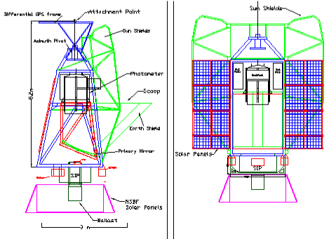
Figure 11: The Boomerang Payload in the LDB configuration. (From [136] with permission.)

The first results [137] were based on the data of a single detector at 150 GHz, while a more detailed analysis covering four 150 GHz detectors and a larger data set was later presented [297] including a refined estimate of beam shape reconstruction and calibration. The most significant residual systematic uncertainty at large multipoles came from the poor knowledge of the effective beam sizes, which in turn was affected by pointing uncertainties (of order of 2.5^′). Extragalactic sources as well as some bright galactic HII regions were used to map the beams ($\sim 18^{\prime}$ at 90 GHz, $\sim 9.5^{\prime}$ at 150 GHz, $\sim 14^{\prime}$ at 240 GHz, and $\sim 12^{\prime}$ at 410 GHz). To map the near sidelobes, azimuthal near-field cuts were measured down to $-20$ dB, but discrepancies of order 10% between the modelled and measured beams were found for the multi-mode Winston concentrators. The window function was generated based on physical optics models of the far field patterns. The observed sky patch was chosen to avoid the Galactic plane and to include some selected point sources. Calibration at 150 GHz was obtained using the CMB dipole. The second analysis [158] lead to a 10% correction in the power spectrum calibration with respect to the first one [137].

A powerful test against systematic effects was to difference the map made from data acquired in the first half of the flight with a scan velocity of 2^∘/sec from that of the second half of the flight at 1^∘/second. Such difference map is sensitive to solar and ground contamination. One of the 150 GHz channels was found to be contaminated and was not used in the analysis. The same test was applied to the combination of the 150 GHz channels, leading to a residual at $\ell<400$ of $\sim 7$ $\mu$K, possibly due to atmospheric contamination.

The Boomerang results lead to the first robust and self-consistent measurement of the first acoustic peak and probed the power spectrum in the range $75<\ell<1025$: it thus represented a major breakthrough in the field. Fits to Boomerang data to estimate cosmological parameters [298, 297] indicate that with the prior assumption $0.45<h<0.90$ the values of both $\Omega_{0}$ and $n_{S}$ were strongly constrained to be close to unity, and supported values of $\Omega_{b}$ consistent with those suggested by cosmological nucleosynthesis [48]. Taking into account large scale structure observations and supernovae Type 1a light curves, the constraints were even more powerful. The best estimate for the Hubble parameter was $h=0.68\pm 0.09$, in excellent agreement with the results of the Hubble Space Telescope key project [299] of $h=0.72\pm 0.08$, and strong evidence for the existence of dark matter and dark energy was found with $\Omega_{\Lambda}\approx 0.7$ and $\Omega_{m}\approx 0.3$.

7.3.8 Maxima

A follow-up of the MAX project, the Maxima collaboration involves U.C. Berkeley, the University of Minnesota/Twin Cities, CalTech, University of Rome, and the IROE-CNR in Florence. The experiment [300] was a balloon-borne bolometric receiver sensitive to multipoles $80<\ell<800$. The receiver housed 16 bolometric channels (compared to the single photometer of MAX) with frequency bands centred at 150, 240, and 410 GHz. The bolometers were cooled to 100 mK, by an adiabatic demagnetisation refrigerator, and a pumped ³He stage provided an intermediate temperature of 300 mK. The focal assembly was coupled to a 1.3 m diameter off-axis Gregorian telescope, yielding a typical angular resolution of $\sim 10^{\prime}$. The warm secondary mirror used in the MAX experiment was replaced with cold secondary and tertiary mirrors, which allowed to insert a cold baffle in the optical path. To reduce the effects of temperature gradients on the optics, the large primary mirror, rather than the secondary, was modulated such that the optical beam on the primary remained stationary.

The first flight in its full configuration [21] was launched in August 1998, and produced one of the most important data sets together with the Boomerang results. A 124 deg² sky region (0.3% of the sky, 3200 independent pixels) was imaged during the 7-hour flight in a direction near Draco with low galactic dust contamination. The data were calibrated using in-flight measurements of the CMB dipole. A map of the CMB anisotropy obtained by combining 150 and 240 GHz data, without foreground subtraction, yielded angular information in the range $36<\ell<785$. The spectrum showed clear evidence of a peak with an amplitude of $78\pm 6$ $\mu$K at $\ell\sim 220$ and an amplitude varying between $\sim 40$ and $\sim 50$ $\mu$K for $400<\ell<785$.

Recently [256] the analysis of the first flight was extended to smaller angular scales, up to $\ell=1235$, using data from three 150 GHz channels in the central 60 deg² of the map. The results of the new analysis, which used improved resolution in the map making, were consistent with the findings of [155] for $\ell<785$. For higher multipoles, evidence was found of excess power at $\ell\sim 860$ over the average level at $411<\ell<785$, suggesting the presence of a third acoustic peak [301]. At the same time the observed power spectrum was found not consistent [301] with a number of the non-standard (but still inflation-based) models that have been proposed to improve the quality of fits to the overall CMB data set. Combined with the $COBE$-DMR data, the Maxima map gave best fit values for a number of cosmological parameters; in particular, for the baryon density, $\Omega_{b}h^{2}\simeq 0.0325{\pm 0.0125}$, and the total density, $\Omega_{0}=0.9{+0.18\atop-0.16}$ (95% confidence level). Gaussianity tests were also performed [302] leading to upper limits to possible deviations at scales between 10^∘ and 5^∘.

7.4 Summary and discussion of up-to-date CMB measurements

Tables 7.4 though 7.4 contain information about various experimental features and results of those measurements leading to anisotropy detection.

Summary of CMB experiments and detection reported in Fig. 12 Name Type ^a /Tech.^b $\theta$,$f_{\rm sky}$ $\nu$ ^c $T_{\rm det}$ Calibr. $\ell\pm\Delta\ell$ $\delta T_{\ell}$ Altitude [GHz] [K] [$\mu$K] $DMR$ S/R $7^{\circ}$ 31.5 290^d 0.7% 2.1${}^{+0.4}_{-0.1}$ 8.5${}^{+16.0}_{-8.5}$ 900 km 100% 53 140^e S/C motion 3.1${}^{+0.6}_{-0.6}$ 28.0${}_{-10.3}^{+7.5}$ 90 Moon 4.1${}^{+0.7}_{-0.7}$ 34.0${}^{+6.0}_{-7.2}$ Internal 5.6${}^{+1.0}_{-0.9}$ 25.1${}^{+5.3}_{-6.6}$ 8.0${}^{+1.3}_{-1.2}$ 29.4${}^{+3.6}_{-4.1}$ 10.9${}^{+1.3}_{-1.2}$ 27.7${}_{-4.5}^{+3.9}$ 14.3${}^{+1.3}_{-1.6}$ 26.1${}_{-5.2}^{+4.4}$ 19.4${}^{+2.7}_{-2.8}$ 33.0${}_{-5.4}^{+4.6}$ Tenerife G/R $5.1^{\circ}$ 10.4 70 … 20.0${}^{+10.0}_{-8.0}$ 32.5${}^{+10.1}_{-8.5}$ 2400 m 15% 14.9 Moon 33 Sun Gal. plane FIRS B/B 3.8^∘ 170 0.24 … 11.0${}^{+17.0}_{-9.0}$ 29.4${}^{+7.8}_{-7.7}$ 35 km 25% 290 Dipole 3.1${}^{+0.6}_{-0.6}$ 28.0${}_{-10.3}^{+7.5}$ 500 Internal 4.1${}^{+0.7}_{-0.7}$ 34.0${}^{+6.0}_{-7.2}$ 680 IACB G/B 2^∘ 91 0.33 5-25%^f 33.0${}^{+26.0}_{-16.0}$ 111.9${}^{+65.4}_{-60.1}$ 2400 m 0.5% 142 Moon 53.0${}^{+26.0}_{-19.0}$ 54.6${}^{+27.2}_{-21.9}$ 230 273 IAC G/B 1.35^∘ 96-270 0.33 10% 39.0${}^{+38.0}_{-24.0}$ 34.0${}^{+8.0}_{-6.0}$ 2400 m 2.4% Moon 61.0${}^{+28.0}_{-22.0}$ 40.0${}^{+7.0}_{-6.0}$ 81.0${}^{+27.0}_{-20.0}$ 41.0${}^{+8.0}_{-8.0}$ 99.0${}^{+24.0}_{-18.0}$ 50.0${}^{+10.0}_{-9.0}$ 116.0${}^{+23.0}_{-14.0}$ 46.0${}^{+10.0}_{-9.0}$ 134.0${}^{+20.0}_{-22.0}$ 56.0${}^{+11.0}_{-10.0}$ SP G/R 1.5^∘ 38-45 4 10% 61.0${}^{+41.0}_{-31.0}$ 30.2${}^{+8.9}_{-5.5}$ 2800 m Moon 61.0${}^{+41.0}_{-31.0}$ 36.3${}^{+13.6}_{-6.1}$ Internal Saskatoon G/R 1.04^∘ 26-46 20 13% 87.0${}^{+44.0}_{-35.0}$ 49.0${}^{+8.0}_{-5.0}$ 480 m 1.42^∘ Cas-A 166.0${}^{+39.0}_{-48.0}$ 69.0${}^{+7.0}_{-6.0}$ 0.5% 237.0${}^{+36.0}_{-48.0}$ 85.0${}^{+10.0}_{-8.0}$ 286.0${}^{+33.0}_{-44.0}$ 86.0${}^{+12.0}_{-10.0}$ 349.0${}^{+51.0}_{-46.0}$ 69.0${}^{+19.0}_{-28.0}$ JB-IAC G/R-I 1^∘ 33 20 6.6% 109${}^{+19.0}_{-19.0}$ 43.0${}^{+12.0}_{-12.0}$ 2800 m 0.8% Moon Tau-A

• S = Space, G = Ground, B = Balloon

• R = Radiometer, B = Bolometer, I = Interferometer

• Where a frequency range is indicated (e.g. 26-46) then the receiver operated in a wide frequency band. See text for further detail.

• 31.5 GHz radiometers.

• 53 and 90 GHz radiometers

• Depending on frequency

Summary of CMB experiments and detection reported in Fig. 12. Continued Name Type/Tech. $\theta$,$f_{\rm sky}$^a $\nu$ $T_{\rm det}$ Calibr. $\ell\pm\Delta\ell$ $\delta T_{\ell}$ [GHz] [K] [$\mu$K] QMAP B/R 54^′ 31 2.3 10-13% 80.0${}^{+41.0}_{-41.0}$ 47.0${}^{+6.0}_{-7.0}$ 30 km 42^′ 42 Cas-A 110.0${}^{+65.0}_{-63.0}$ 52.0${}^{+5.0}_{-5.0}$ 0.2% 126.0${}^{+54.0}_{-54.0}$ 59.0${}^{+6.0}_{-7.0}$ ARGO B/B 52^′ 150 0.28 10% 95.0${}^{78.0}_{-44.0}$ 39.1${}^{+8.7}_{-8.7}$ 35 km (65) 250 Internal 95.0${}^{78.0}_{-44.0}$ 46.8${}^{+9.5}_{-12.1}$ 375 95.0${}^{78.0}_{-44.0}$ 46.8${}^{+9.5}_{-12.1}$ 600 95.0${}^{78.0}_{-44.0}$ 46.8${}^{+9.5}_{-12.1}$ Python G/R-B 45^′-1^∘ 40 11^b 15-20% 88.0${}^{+17.0}_{-39.0}$ 60.0${}^{+15.0}_{-13.0}$ 2800 m 0.3% 90 0.5^c Internal 170.0${}^{+69.0}_{-50.0}$ 66.0${}^{+17.0}_{-16.0}$ Python V G/R $\sim 1^{\circ}$ 37-45 12-15% 44.0${}^{+25.0}_{-15.0}$ 22.0${}^{+4.0}_{-5.0}$ 2800 m 1.44% Internal 75.0${}^{+15.0}_{-15.0}$ 24.0${}^{+6.0}_{-7.0}$ 106.0${}^{+15.0}_{-15.0}$ 34.0${}^{+7.0}_{-9.0}$ 137.0${}^{+15.0}_{-15.0}$ 50.0${}^{+9.0}_{-23.0}$ 168.0${}^{+15.0}_{-15.0}$ 61.0${}^{+13.0}_{-17.0}$ 199.0${}^{+15.0}_{-15.0}$ 77.0${}^{+20.0}_{-28.0}$ BAM B/B 42^′ 110-250 0.26 20% 74.0${}^{+82.0}_{-47.0}$ 55.6${}^{+29.6}_{-15.2}$ 41.4 km (10) Jupiter TOCO97 G/R 42^′c 31 36 ^d 5% 63.0${}^{+18.0}_{-18.0}$ 40.0${}^{+10.0}_{-9.0}$ 5240 m 42 Jupiter 86.0${}^{+16.0}_{-22.0}$ 45.0${}^{+7.0}_{-6.0}$ 15^′ 144 4 114.0${}^{+20.0}_{-24.0}$ 70.0${}^{+6.0}_{-6.0}$ 1.45% 158.0${}^{+22.0}_{-23.0}$ 89.0${}^{+7.0}_{-7.0}$ 199.0${}^{+38.0}_{-29.0}$ 85.0${}^{+8.0}_{-8.0}$ TOCO98 128.0${}^{+26.0}_{-33.0}$ 55.0${}^{+18.0}_{-17.0}$ 152.0${}^{+26.0}_{-38.0}$ 82.0${}^{+11.0}_{-11.0}$ 226.0${}^{+37.0}_{-56.0}$ 83.0${}^{+7.0}_{-8.0}$ 306${}^{+44.0}_{-59.0}$ 70.0${}^{+10.0}_{-11.0}$ MAX B/B 30^′ 105 0.28 ^e 10% 139.0${}^{+108.0}_{-67.0}$ 49.4${}^{+7.8}_{-7.8}$ 36 km (5) 180 0.085 Venus 270 Jupiter 360 Internal

• Number in parenthesis indicates number of pixels.

• 11 K for 40 GHz radiometer, 0.5 K for 90 GHz bolometer

• 42^′ at Ka and Q bands, 15^′ at D band.

• Front-end HEMTS at 36 K, SIS mixers at 4 K.

• 0.28 K first and second flight, 0.085 K third and fourth flight.

Summary of CMB experiments and detection reported in Fig. 12. Continued Name Type/Tech. $\theta$,$f_{\rm sky}$ $\nu$ $T_{\rm det}$ Calibr. $\ell\pm\Delta\ell$ $\delta T_{\ell}$ [GHz] [K] [$\mu$K] CAT G/R-I 30^′ 13-17 17 10% 397.0${}^{+84.0}_{-65.0}$ 50.8${}^{+15.4}_{-15.4}$ Sea-level 0.02% Cas-A 615.0${}^{+102.0}_{-72.0}$ 49.0${}^{+19.1}_{-13.6}$ 391.0${}^{+84.0}_{-65.0}$ 54.0${}^{+9.5}_{-6.4}$ 615.0${}^{+102.0}_{-72.0}$ 43.6${}^{+13.6}_{-13.1}$ MSAM B/B 28^′ 170 0.24 11% 84.0${}^{+46.0}_{-45.0}$ 35.0${}^{+15.0}_{-11.0}$ 39.5 km 0.02% 180 Jupiter 201.0${}^{+82.0}_{-70.0}$ 49.0${}^{+10.0}_{-8.0}$ 415 407.0${}^{+46.0}_{-123.0}$ 47.0${}^{+7.0}_{-6.0}$ 678 DASI G/R-I 20^′ 26-36 20 7% 118.0${}^{+49.0}_{-14.0}$ 61.4${}^{+6.3}_{-7.1}$ 2800 m 0.9% Internal 203.0${}^{+52.0}_{-30.0}$ 72.7${}^{+4.4}_{-3.9}$ 289.0${}^{+53.0}_{-28.0}$ 60.5${}^{+2.7}_{-2.9}$ 377.0${}^{+41.0}_{-35.0}$ 40.6${}^{+2.4}_{-2.5}$ 465.0${}^{+35.0}_{-47.0}$ 43.4${}^{+2.5}_{-2.6}$ 553.0${}^{+41.0}_{-47.0}$ 53.3${}^{+2.6}_{-2.8}$ 641.0${}^{+35.0}_{-41.0}$ 40.8${}^{+3.2}_{-3.6}$ 725.0${}^{+32.0}_{-49.0}$ 44.8${}^{+3.8}_{-4.1}$ 837.0${}^{+27.0}_{-74.0}$ 48.2${}^{+4.4}_{-4.9}$ Viper G/R 16^′ 38 20 8% 108.0${}^{+121.0}_{-78.0}$ 61.6${}^{+31.1}_{-21.3}$ 2800 m … 45 Internal 173.0${}^{+114.0}_{-101.0}$ 77.6${}^{+26.8}_{-19.1}$ 237.0${}^{+99.0}_{-111.0}$ 66.0${}^{+24.4}_{-17.2}$ 263.0${}^{+185.0}_{-113.0}$ 80.4${}^{+18.0}_{-14.2}$ 422.0${}^{+182.0}_{-131.0}$ 30.6${}^{+13.6}_{-13.2}$ 589.0${}^{+207.0}_{-141.0}$ 65.8${}^{+25.7}_{-24.9}$ Maxima B/B 10^′ 150 0.1 4% 77.0${}^{+33.0}_{-41.0}$ 45.0${}_{-6.0}^{+7.0}$ 38.4 km 0.3% 240 Dipole 147.0${}^{+38.0}_{-36.0}$ 54.0${}_{-5.0}^{+6.0}$ 410 222.0${}^{+38.0}_{-74.0}$ 78.0${}_{-6.0}^{+6.0}$ 294.0${}^{+41.0}_{-33.0}$ 62.0${}_{-5.0}^{+5.0}$ 381.0${}^{+29.0}_{-45.0}$ 48.0${}_{-5.0}^{+6.0}$ 449.0${}^{+36.0}_{-38.0}$ 38.0${}_{-4.0}^{+5.0}$ 523.0${}^{+37.0}_{-37.0}$ 44.0${}_{-5.0}^{+5.0}$ 597.0${}^{+38.0}_{-36.0}$ 43.0${}_{-6.0}^{+6.0}$ 671.0${}^{+39.0}_{-35.0}$ 46.0${}_{-6.0}^{+6.0}$ 746.0${}^{+39.0}_{-35.0}$ 47.0${}_{-8.0}^{+8.0}$ 856.0${}^{+79.0}_{-70.0}$ 56.0${}^{+7.0}_{-7.0}$ 1004.0${}^{+81.0}_{-68.0}$ 33.0${}_{-22.0}^{+13.0}$ 1147.0${}^{+88.0}_{-61.0}$ 15.0${}_{-15.0}^{+29.0}$

Summary of CMB experiments and detection reported in Fig. 12. Continued Name Type/Tech. $\theta$,$f_{\rm sky}$ $\nu$ $T_{\rm det}$ Calibr. $\ell\pm\Delta\ell$ $\delta T_{\ell}$ [GHz] [K] [$\mu$K] Boomerang B/B 10^′ 90 0.28 10% 101.0${}^{+24.0}_{-25.0}$ 59.3${}^{+4.5}_{-4.9}$ 29 km 1.8% 150 Dipole 151.0${}^{+24.0}_{-25.0}$ 68.5${}^{+3.9}_{-4.2}$ 240 201.0${}^{+24.0}_{-25.0}$ 74.7${}^{+3.6}_{-3.7}$ 410 251.0${}^{+24.0}_{-25.0}$ 75.5${}^{+3.1}_{-3.3}$ 301.0${}^{+24.0}_{-25.0}$ 62.3${}^{+2.5}_{-2.5}$ 351.0${}^{+24.0}_{-25.0}$ 50.9${}^{+2.0}_{-2.1}$ 401.0${}^{+24.0}_{-25.0}$ 42.9${}^{+1.7}_{-1.8}$ 451.0${}^{+24.0}_{-25.0}$ 45.5${}^{+1.7}_{-1.8}$ 501.0${}^{+24.0}_{-25.0}$ 47.6${}^{+1.8}_{-1.9}$ 551.0${}^{+24.0}_{-25.0}$ 47.8${}^{+2.1}_{-1.9}$ 601.0${}^{+24.0}_{-25.0}$ 45.3${}^{+2.0}_{-2.0}$ 651.0${}^{+24.0}_{-25.0}$ 44.0${}^{+2.1}_{-2.3}$ 701.0${}^{+24.0}_{-25.0}$ 42.7${}^{+2.4}_{-2.5}$ 751.0${}^{+24.0}_{-25.0}$ 37.9${}^{+2.9}_{-3.1}$ 801.0${}^{+24.0}_{-25.0}$ 43.8${}^{+3.1}_{-3.4}$ 851.0${}^{+24.0}_{-25.0}$ 47.3${}^{+3.7}_{-3.9}$ 901.0${}^{+24.0}_{-25.0}$ 41.8${}^{+4.9}_{-5.4}$ 951.0${}^{+24.0}_{-25.0}$ 31.3${}^{+7.3}_{-9.4}$ 1001.0${}^{+24.0}_{-25.0}$ 22.4${}^{11.4}_{-22.4}$ CBI G/R-I 5^′ 26-36 6 5% 603${}^{+180.0}_{-166}$ 58.7${}_{-6.3}^{+7.7}$ 5080 m 0.1% Jupiter 1190${}^{+261.0}_{-224}$ 29.7${}_{-4.2}^{+4.8}$ Tau-A CBI-2 G/R-I 5^′ 26-36 6 5% 200${}^{+100.0}_{-200.0}$ 72.4${}^{+13.7}_{-16.9}$ 5080 m 0.1% Jupiter 407${}^{+93.0}_{-107.0}$ 44.7${}^{+5.0}_{-5.7}$ Tau-A 605${}^{+95.0}_{-105.0}$ 45.5${}^{+3.9}_{-4.4}$ 801${}^{+99.0}_{-101.0}$ 50.3${}^{+3.8}_{-4.1}$ 1002${}^{+98.0}_{-102.0}$ 29.3${}^{+3.9}_{-4.4}$ 1197${}^{+103.0}_{-97.0}$ 35.4${}^{+3.8}_{-4.2}$ 1395${}^{+105.0}_{-95.0}$ 21.6${}^{+5.4}_{-7.4}$ 1597${}^{+103.0}_{-97.0}$ 26.7${}^{+5.5}_{-6.9}$ OVRO G/R 22^′-7.4^′a 14.5 … 4.3% 537.0${}^{+267.0}_{-205.0}$ 56.0${}^{+8.5}_{-6.6}$ 1200 m 31.7 Jupiter Cas-A

• Depending on frequency.

All the power spectrum measurements are plotted in Fig. 12. To obtain a clearer view of the observational status and to check for self-consistency of the detections, we have combined different results in a limited number of $\Delta\ell$ intervals. We considered separately ground-based and balloon-borne results, which are characterised by widely different potential systematic errors. In fact, in addition to the different observing environments, these two categories typically represent independent instrumental approaches and contaminated by different astrophysical foregrounds. As it emerges from the discussion of the various experiments in the previous sections, almost all balloon experiments (with the exception of QMAP) exploited, in the relatively short flight-time available, the excellent sensitivity of bolometric detectors at sub-mm wavelengths; while most ground-based instruments (besides IAC, IAC-B and the 90 GHz channel of Python) employed HEMT-based receivers, which are best suited for ground observations in the low-frequency ($<100$ GHz) atmospheric windows (see Sections 4.4 and 4.7). As a consequence of the frequency split, different foreground components (see Section 3) dominate the two subsets of measurements.

To combine the subsets of data, we followed the technique described in [303]. Let $\mathbf{y}$ be a vector of CMB detections (expressed in terms of $\delta T^{2}$). The assumed data model is

$$\mathbf{y}=\mathbf{Wx}+\mathbf{n}\,,$$ (51)

where $\mathbf{x}$ is the “true” power spectrum up to a fiducial high multipole $\ell_{\rm max}$ (we assume here $\ell_{\rm max}=2000$), $\mathbf{W}$ is the window function for each detection. The instrument error is assumed to be a random variable with zero mean ($\langle\mathbf{n}\rangle=0$) with a variance given by $\mathbf{N}\equiv\langle\mathbf{nn}^{t}\rangle$, that is the sum of four different sources of error:

$$\mathbf{N}=\mathbf{N}^{\rm meas}+\mathbf{N}^{\rm scal}+\mathbf{N}^{\rm ical}+\mathbf{N}^{\rm beam}\,,$$ (52)

where the first term is the quoted error in the measured $\delta T^{2}$, the other terms account for the uncertainty in the calibration source ($\mathbf{N}^{\rm scal}$), for the calibration uncertainty specific of each single experiment ($\mathbf{N}^{\rm ical}$) and for the beam uncertainty. In general all these errors will depend upon the actual power spectrum $\mathbf{x}$. We however make the approximation that relative errors are small and therefore in this limit the matrix $\mathbf{N}$ is independent of $\mathbf{x}$. If $\mathbf{W}$, $\mathbf{N}$ and $\mathbf{y}$ are known, it is straightforward to invert the problem and obtain the true power spectrum. Note that, from a mathematical point of view, this is identical to the map-making problem (see Sect. 6.1). In this case, however, the dimensions of the problem are such that it can be easily treated numerically. Therefore the best, minimum-variance estimator $\mathbf{\hat{x}}$ of the underlying power spectrum $\mathbf{x}$ is given by:

$$\mathbf{\hat{x}}\equiv[\mathbf{W}^{t}\mathbf{N}^{-1}\mathbf{W}]^{-1}\mathbf{W}^{t}\mathbf{N}^{-1}\mathbf{y}\,.$$ (53)

For the map-making problem, this solution is known to be minimum variance and un-biased. Instead of considering the true power spectrum $\mathbf{x}$ as an independent parameter in each multipole, we treated the power as a piecewise constant simply parameterised by its height $x_{i}$ in a suitable number of bands in $\ell$-space. Furthermore, since our band-power estimator $\mathbf{\hat{x}}$ is a linear combination of the input data, it is possible to obtain the window function relative to each band-power taking the same linear combination of the input matrix $\mathbf{W}$. From these band-power window functions we derived the horizontal bars and the mean point taken to be respectively the 20, 80 and 50% quantile, respectively, of the absolute value of the band-power window function.

Fig. 13 shows the results for the CMB detections divided in ground-based, balloon-borne and space ($COBE$-DMR) experiments. Both ground and balloon results show, independently, clear evidence of the acoustic pattern of the power spectrum and in particular of the first two peaks, located approximately at $\ell\sim 200$ and $\ell\sim 500$, respectively. A third peak near $\ell\sim 800$ is also suggested by both data sets. This general agreement is a noteworthy result, and provides strong indication that the systematic effects and residual foreground errors that affect the current set of observations, while representing one of the main sources of uncertainty, do not dominate the basic features observed in the power spectrum. On the other hand, it is also clear that much room exists to improve the current precision in measurements of the angular power spectrum.

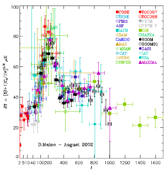
Figure 12: The full set of CMB anisotropy measurements, as described in Sect. 7.

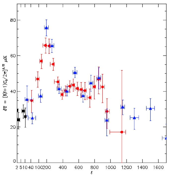
Figure 13: Anisotropy detections combined in a limited number of intervals. Black data points: $COBE$-DMR results; Red data points: balloon-borne (mostly bolometers, $\nu>100$ GHz) experiments; Blue data points: ground-based (mostly radiometers, $\nu<100$ GHz) experiments. Ground-based data extends up to higher $\ell$’s thanks to the recent results from the CBI experiment.

8 ONGOING AND PLANNED EXPERIMENTS

Further observing campaigns are now on-going for several of the programs described in Sect. 7, such as Boomerang, Maxima, CBI, DASI. In addition a number of new ambitious sub-orbital projects are currently being planned for the near future, either as continuation of existing collaborations or as new enterprises. The forthcoming results of the $MAP$ mission, to be released within one year, are expected to over-ride many of the current anisotropy results, and will certainly make it much harder for traditional ground-based and balloon-borne experiments to be competitive. The Planck maps, expected in the second half of this decade, will definitively cover the whole sky with exquisite precision and spectral coverage, pushing out of date most of the current experimental approaches. On the other hand, we do not believe that Planck will represent an end for CMB observations, but rather the starting point of a new phase (see Sect. 9.1). In fact, some of the experiments currently being designed include features that may anticipate future developments; in particular increasing emphasis is given to very high resolution and to polarisation capabilities.

8.1 Temperature anisotropy projects

Two projects in the high ($>100$ GHz) and low ($<100$ GHz) frequency regimes, Archeops and BEAST, are being carried out as precursors of the Planck LFI and HFI instruments, respectively. Archeops is a balloon-borne bolometric instrument with angular resolution $\sim 8^{\prime}$, eventually intended to cover $\sim 25\%$ of the sky at 143, 217, 353 and 545 GHz. The bolometers cooled to 0.1 K can provide sensitivity to CMB fluctuations of 100 $\mu$K in as many as $9\times 10^{4}$ pixels with FWHM$\sim 20^{\prime}$. Results from a test flight from Trapani (Sicily) to Spain in July 1999 are described by [304], while data from a second flight are now being analysed. The BEAST instrument is operated in its present configuration in Ka and Q band, using LFI-like focal plane and components [106]. The program, carried out by a collaboration involving UCSB, JPL, Italian groups in Milano, Bologna and Roma and INPE-Brazil, has been flown twice and, in addition, now large amounts of data covering $\sim 3000$ deg² with $20^{\prime}$ have been collected from the White Mountain High Altitude Station, California (3800 m) and the analysis is being completed as we write. Future plans include the addition of a W band polarisation channel and to fly the experiment as a LDB balloon. Eventually it may be possible to fly the payload as a ultra long duration ($>100$ days) flight, a possibility technically feasible.

When approaching excellent instrument sensitivities, the main source of concern tends to become the control of systematic errors rather than sheer sensitivity. This is a crucial issue in view of the future development of precision CMB imaging. For example, to create an observing environment maximally free from local stray radiation a novel instrument concept was proposed for the TopHat experiment [305], a bolometer-based long duration balloon project in which the instrument is located on top of the balloon rather than hanging below it. With this arrangement, the entire sky above the instrument is free from supporting structures which could scatter radiation into the sidelobes of the optics.

Most ground based projects currently active or planned are based on interferometer instruments. Among them is the Very Small Array (VSA), now taking data from Tenerife. The project is a collaboration between MRAO, NRAL and IAC. The VSA design includes an array of 14 horn-reflector antennas in a T-shaped configuration, and it represents a second-generation after the CAT interferometer. The VSA aims at obtaining detailed maps with angular sensitivity between $10^{\prime}$ and $2^{\circ}$ with $\sim 5$ $\mu$K noise in 4 frequency bands in the 28–37 GHz range. Another interferometer experiment called AMiBA (Array for Microwave Background Anisotropy), is expected to be operative by 2003 [307, 308]. This will be a 19 elements, W-band array by the Academia Sinica, Institute of Astronomy and Astrophysics, and National University of Taiwan, devoted to CMB polarisation and S-Z effect observation.

Antarctic winter observations may also have a long future. The Arcminute Cosmology Bolometer Array Receiver (ACBAR) is a 16 element array of bolometers cooled at 0.23 K designed for observation of small scale anisotropy and Sunyaev-Zeldovich effect. The experiment, run by the Center for Astrophysical Research in Antarctica (CARA), was deployed at the South Pole in December 2000. Preliminary results in the range $200<\ell<2200$ based on data taken in the austral winter of 2001 were presented [309] including serendipitous discoveries of high redshift clusters via their S-Z effect.

To gain the angular resolution needed to probe fine structures, existing radio-telescopes may be employed if properly adapted. It has been proposed [310] to use the Ratan-600, the large Russian radio telescope, coupled with high sensitivity receivers for CMB anisotropy and polarisation measurements. The so-called “Cosmological Gene” main frequency would be 32 GHz, with a set of frequencies in the 1-22 GHz range for foreground subtraction. Very high angular resolution ($\sim 1^{\prime}$) is in principle obtainable provided that the optics quality and atmospheric conditions are adequate.

8.2 Polarisation anisotropy projects

An increasing number of projects are designed to attempt polarisation detection. Early work [311, 312, 313, 224] has confirmed the low level of polarisation expected in the CMB signal. Despite the increasing experimental effort [314, 315, 316, 317, 318], up to now only upper limits have been obtained, constraining CMB polarisation at the 10 $\mu$K level. A complete discussion of CMB polarisation experiments is out of the scope of this work. However, it is clear that the trend for most CMB anisotropy projects is to include polarisation capability.

At large angular scales ($\ell\leq 200$) theory predicts a CMB polarised component as weak as sub-$\mu$K level (see Fig. 1), far lower than the sensitivities currently achieved even by the most advanced instruments. An attempt to reach a statistical detection at large scales was carried out with the POLAR correlation radiometer [318] using HEMTs in Ka band cooled to 15 K. Sensitivities of few $\mu$K in $\sim 30$ pixels could be obtained in several months of observing time. Analysis of the $\sim 750$ hours of data lead to upper limits $\sim 10$ $\mu$K. A space experiment to search for polarisation at $>7^{\circ}$ scales is the SPORT project [320, 321, 322] proposed for implementation on the International Space Station. The instrument is based on HEMT radiometers cooled to $\sim 90$ K and operating at 4 frequencies in the 20-90 GHz range. A nearly full sky map can be obtained with a sensitivity of $\sim 5$ $\mu$K per $7^{\circ}$ resolution element, which is adequate for a valuable measurement of the Galactic polarised emission. The balloon-borne counterpart of SPORT, called BarSport, has a multi-feed focal plane of polarimeters in W band at the focus of an on-axis telescope reaching sub-degree angular resolution in small sky patches [323].

A number of ground-based and balloon borne experiments exploiting the novel technique of polarisation sensitive bolometers (PSBs; see Sect 4.7) are being planned. A new circum-Antarctic LDF flight (B2K) is being prepared for Boomerang, with the aim of detecting CMB polarisation [324] using PSBs at frequencies 150, 245 and 345 GHz. In addition to polarisation capability, the instrument has improved attitude reconstruction (a main limiting factor in the first Boomerang flight) and calibration (goal precision better than 1%). QUEST (Q and U Extragalactic Sub-mm Telescope) is another CMB polarimetric instrument being designed and built at Cardiff and Caltech [325]. The QUEST on-axis Cassegrain optics will produce $1.5^{\circ}$ images with $\sim 5^{\prime}$ resolution with multi-element arrays of polarisation sensitive bolometers at 100, 150, and 220 GHz. A ground-based bolometric receiver with polarisation capability, Polatron, is being developed for use at the Owens Valley 5.5 meter radio telescope. The scanning strategy and experimental design will be similar to the SuZIE experiment, while the single-mode feed structure and spider-web bolometers will be similar to those of Boomerang. The experiment is designed to run autonomously to cover long integration times. For this reason, the cryogenic chain (with a 4 K stage provided by a mechanical cryocooler, and a 0.25 K stage by a multi-stage sorption cooler) will consume no liquid cryogens.

8.3 Towards precision CMB imaging

Soon after the $COBE$-DMR detection [15] it become clear that a reasonable extrapolation into the future of millimetre-wave technology could support high-sensitivity, sub-degree surveys of large portions of the sky. At the same time, the unique scientific potential of extended high resolution observations became widely recognised. While several ground and balloon experiments were being prepared, a few groups proposed space projects to fully accomplish the pioneering work of $COBE$ (e.g. [326, 327, 328, 329, 330, 331, 332]). After detailed assessment studies and competitive peer reviews, in 1996 two CMB missions were selected for implementation: NASA’s Microwave Anisotropy Probe ($MAP$) and ESA’s Planck Surveyor (formerly known as COBRAS/SAMBA). The $MAP$ mission was launched in June 2001, it is currently observing and the first data are expected in early 2003. $MAP$ will provide a major step forward in the power spectrum determination with respect to all the present sub-orbital experiments. The Planck mission is designed to fully extract the cosmological information contained in CMB anisotropy by setting angular resolution, spectral coverage and sensitivity such that the power spectrum reconstruction will be limited by unavoidable cosmic variance and astrophysical foregrounds. Both missions are also sensitive to linear polarisation at proportional levels. Table 8.3 summarises the main performances of $MAP$ and Planck.

Main instrumental performances of the MAP and Planck missions. $MAP$ Planck LFI HFI Angular resolution 14^′–56^′ 33^′–10^′ 9.2^′–5^′ Avg. $\Delta T/T$ per pixel^a Intensity 4.0 $\times 10^{-5}$ 6.6$\times 10^{-6}$ 2.0$\times 10^{-6}$ (1 year mission)^b Polaris.^c 5.6$\times 10^{-5}$ 9.3$\times 10^{-6}$ 4.2$\times 10^{-6}$ Baseline mission lifetime 2 years^d 14 months 14 months Spectral coverage 22–90 GHz 30–100 GHz 100–857 GHz Detector technology HEMT HEMT Bolometers Detector temperature $\sim 90$ K 20 K 0.1 K Cooling Passive Active Active

• The sensitivity in thermodynamic temperature and refers to the W-band detectors (94 GHz for MAP and 100 GHz for Planck) on a 10^′ pixel. A pixel is a square whose side is the FWHM extent of the beam.

• These figures are calculated for the average integration time per pixel. In general the integration time will be inhomogeneously distributed on the sky and will be much higher in certain regions of it.

• Refers to E-mode polarisation (Stokes parameters U and Q).

• Recently the MAP team has requested an extention to 4 years of the mission lifetime.

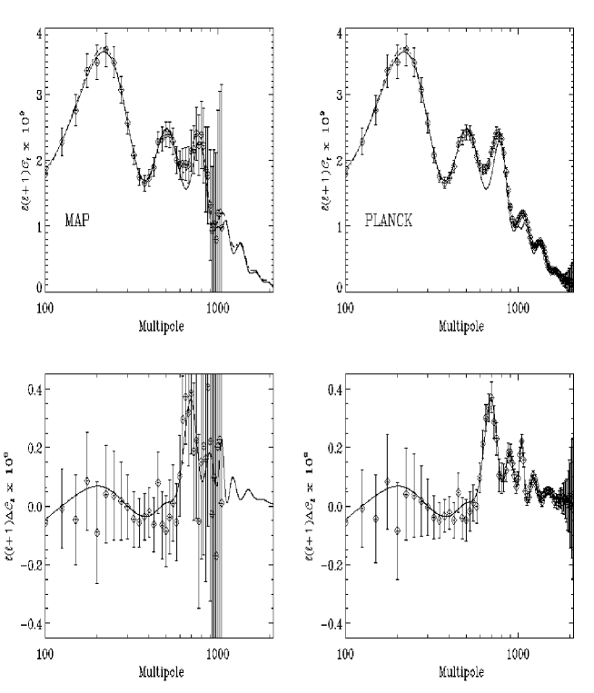
Figure 14: Simulated power spectrum measurements by $MAP$ (left) and Planck (right). The upper panels show two nearly degenerate CDM models (solid and dotted curves) with significantly different parameters. Although barionic density, $\Omega_{b}$, and dark matter density, $\Omega_{\rm CDM}$, differ by as much as 24% and 5% respectively, the two curves are very similar. The residuals are ploted in the lower panels. The error bars are simulated power spectra reconstructions according to the $MAP$ and Planck instrument specifications. Current anisotropy data (see Fig. 13) are completely unable to discriminate the two models. $MAP$ may tentatively distinguish them, while Planck can precisely discriminate between the two scenarios.

The technical challenge posed by these missions is twofold. First, it is necessary to reach very high sensitivity in order to obtain the wanted signal to noise ratio per pixel over the full sky. Given the key requirement of high angular resolution (up to $14^{\prime}$ for $MAP$ and $5^{\prime}$ for Planck), the requirement on instrument sensitivity is great for a reasonable mission lifetime, $\tau_{\rm mission}\approx 1$–4 yrs. From Eq. (29) the noise per 1 second integration time ($\mu$K$\times$Hz^-1/2), is $\Delta T_{1\,{\rm sec}}=k_{r}{T_{\rm sys}+T_{\rm sky}\over\sqrt{\Delta\nu}}$. Therefore to get an ultimate noise per pixel $\delta T_{\rm pix}$, $\Delta T_{1\,{\rm sec}}$ must satisfy $\Delta T_{1\,{\rm sec}}<\delta T_{\rm pix}\sqrt{n_{\rm R}{\tau_{\rm mission}\over N_{\rm pix}}}$. This calls for arrays of detectors ($n_{\rm R}\sim 10$) with state-of-the-art technology and instruments operating at cryogenic temperatures. The $MAP$ radiometers are operated on a passively cooled payload at $\sim$90 K, while Planck will make full use of cryogenic technology, with radiometers cooled at 20 K and bolometric detectors cooled at 0.1 K.

The second challenge is to make sure that the data accuracy is indeed limited by instrument sensitivity. The more ambitious the sensitivity goal, the more stringent the required rejection of systematic effects, which for $MAP$ and Planck must be controlled at $\mu$K level. The space environment, coupled with an appropriate choice of orbit and scanning scheme, provides a unique chance to avoid most of the environmental limitation of sub-orbital experiments such as atmospheric emission, thermal instability, stray light from the earth, sun and moon, and allows full sky coverage. Both $MAP$ and Planck selected Lissajous orbits around the Lagrangian point L2 of the sun-earth system at 1.5 million km from earth. This vantage point offers an exceptionally stable environment for CMB observations (as well as for other missions, such as Herschel or NGST), since the instrument can always maintain an unobstructed view of deep space. The satellites passive thermal design combined with a constant sun angle results in low thermal drift rates ($\sim$mK/hr) unattainable from any platform near earth.

Both $MAP$ and Planck will exploit the CMB dipole as main calibration source, now known to an accuracy of 20 $\mu$K [165]. In addition, the seasonal variation of the dipole amplitude due to satellite motion will further improve absolute calibration. At frequencies $<300$ GHz photometric calibration better than 0.5% can be obtained [328]. The highest frequencies of Planck will rely on measurements of the emission of the Milky Way, calibrated to 1% by $COBE$/FIRAS (of course Planck will be able to use the $MAP$ data for its own calibration). Also, both missions will measure the main beams in-flight using multiple observations of Jupiter, Saturn and Mars.

As shown in Sect. 7, remarkable progress has been achieved by sub-orbital experiments since the first proposal of $MAP$ and Planck, as it was anticipated at that time. However, it is clear that only unobstructed, deep, full-sky surveys can fully exploit the opportunity for precision cosmology offered by CMB observations. In fact, the present positive detections of acoustic peaks in the power spectrum strongly supports optimism in our ability to reach exquisite accuracy in parameter estimation from deep CMB anisotropy observations. Fig. 14 illustrates the capability of the $MAP$ and Planck missions to accurately reconstruct the power spectrum. In particular, the plots show how the high percision measurements by Planck will allow to discriminate between nearly degenerate sets of $C_{\ell}$s.

8.3.1 $MAP$

The Microwave Anisotropy Probe satellite is expected to reconstruct the angular power spectrum up to $\ell\sim 1000$, limited by cosmic variance for $\ell<500$. The project was proposed to NASA as a MidEx mission in June 1995, and one year later hardware manufacturing started based on off-the-shelf components and space qualified technology. In analogy with $COBE$-DMR, $MAP$ uses differential radiometers in the 23–94 GHz range that measure instantaneous temperature differences between two points in the sky. A pair of back-to-back Gregorian telescopes (1.4 m $\times$ 1.6 m primary, and 0.9 m $\times$ 1.0 m sub-reflector) direct two symmetric beams in the sky separated by $\sim 141^{\circ}$. The telescopes are coupled to two symmetric, 10-element arrays of corrugated feed horns connected to differential receivers. Each focal plane array includes 1 feed at 22 and 30 GHz, 2 feeds at 40 and 60 GHz and 4 feeds at 90 GHz. The feed centres occupy a region $\sim 20$ cm in diameter, which corresponds to $\sim 4.5^{\circ}$ projected in the sky. The angular resolution ranges between $\sim 50^{\prime}$ and $\sim 14^{\prime}$, depending on frequency, with typical ellipticity of the beam shapes $\sim 10\%$. The expected sensitivity is $\sim 35$ $\mu$K per $0.3^{\circ}$ pixel at each frequency in a nominal lifetime of two years.

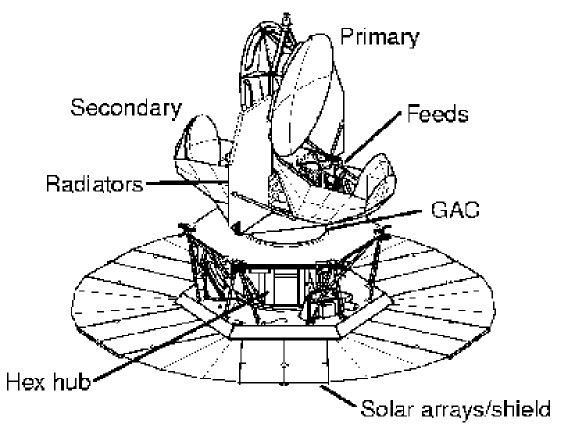
Figure 15: An overview of the $MAP$ satellite, showing the double-telescope system, the large radiators, and the satellite service module with deployable solar panels on the bottom. One of the two focal arrays of feed horns is also partially visible on the right. The overall height is 3.6 m, the mass is 830 Kg and the diameter of the deployed solar panels reaches 5.1 m. The solar arrays supply a 400 Watts power to the spacecraft and instruments. The hexagonal structure (“Hex hub”) above the solar panel array supports the power supply, instrument electronics, and other satellite subsystems. The thermally insulating “gamma alumina cylinder” (GAC) supports a 190 K gradient between the warm and cold portion of the satellite. (With permission, courtesy of the $MAP$ Science Team).

Passive cooling to $\sim 90$ K of the optics and front-end portion of the receivers is ensured by the continuous view of cold space by two large (5.6 m²) radiators, and by separating the front-end and back-end sections of the radiometers. No active cooling is used. Ground tests of the front-end InP HEMT amplifiers [333, 109] achieve noise temperatures of 25-100 K at 80 K [334], and are phase matched over the 17% nominal bandwidth.

After each feed horn, an orthomode transducer separates the two linear polarisations which are processed independently by two differential radiometer chains, thus allowing the system to be sensitive to the linearly polarised component. The sensitivity to the $Q$ and $U$ Stokes parameters is degraded by $\sim\sqrt{2}$ with respect to temperature anisotropy. The receiver scheme is a so-called “pseudo-correlation” receiver [335], in which two hybrid tees and two square-law detectors replace the more traditional multiplier of a typical correlation receiver. A similar design solution was adopted for the Planck-LFI radiometers, where one of the inputs is constituted by an internal cryogenic load. The advantage of these solutions is that they minimise systematic effects due to fluctuations and instabilities of the gain and noise temperature of HEMT amplifiers, typically exhibiting 1/$f$ noise spectrum [130]. In addition, phase switching (at kHz rates) is used to reject low frequency noise from the detector diodes and residual 1/$f$ noise from the back-end.

Large efforts have been made to minimise pixel-to-pixel correlations and many systematic uncertainties that are avoided by design. Possible artifacts in the map-making process are controlled at sub-$\mu$K level. Because of the long time spent in a very stable orbit, and using the observation redundancy of the scan strategy, numerous consistency and systematic checks are possible.

The spacecraft reached L2 using a trajectory with 4 lunar phasing loops followed by a transfer cruise. To satisfy communications requirements and to avoid eclipses, during the Lissajous orbit, the spacecraft-earth vector remains between $1^{\circ}$ and $10^{\circ}$ off the sun-earth vector. The instrument is continuously maintained in the shadow for passive cooling and avoidance of straylight signals. The scan strategy also allows to maintain a constant angle between the sun and the plane of the solar panels for thermal and power stability. The satellite spins at 0.464 rpm ($\sim$2.2 min/spin), and precesses every hour around a $22.5^{\circ}$ cone around the sun-satellite line, which is always within $0.1^{\circ}$ of the sun-earth line. The scan strategy was designed to rapidly scan a large fraction of the sky (30% every day) and to observe each sky pixel through many azimuth angles and at different time scales. The spin and precession periods are out of phase, so that their combined motion causes the observing beams to fill an annulus centred on the local solar vector. As $MAP$ orbits the sun, the annular scan pattern covers the full sky every 6 months, which can be used for long-term stability checks. Algorithms for data analysis and processing of $MAP$-like data have been presented by Wright et al [336], Hinshaw [337], Hivon et al [157].

The multifrequency instrument is designed to disentangle synchrotron and free-free Galactic emission and radio sources. A recent analysis of simulated $MAP$ data at 90 GHz with $0.3^{\circ}$ FWHM [292] showed that foreground contamination on the correlation function is small compared to cosmic variance. However, Galactic emission at $|b|>20^{\circ}$, significantly affects the topology of CMB anisotropy and non-Gaussianity analysis. It was also showed that IRAS and DIRBE far-infrared extragalactic sources have little effect on the CMB anisotropy while radio sources raise the amplitude of the correlation function considerably on scales $<30^{\prime}$. $MAP$ will highly improve over the current measurements of diffuse synchrotron and free-free emissions and polarisation, and the K and Ka bands will be able to verify the possible contribution from spinning dust [338].

In addition to power spectrum measurements, the $MAP$ data can be used for testing Gaussianity and polarisation, in particular for polarisation-temperature cross-correlation. The S-Z effect should be observable in 5 to 10 clusters and possibly also in a few bright extragalactic radio sources.

8.3.2 Planck Surveyor

Following $COBE$-DMR and $MAP$, Planck represents the third generation space mission dedicated to CMB anisotropies. The mission [93, 339] is designed to reach the fundamental limits imposed by cosmic variance and astrophysical foregrounds across the entire power spectrum. The observations will produce 10 full sky maps at frequencies spanning over the CMB blackbody spectrum in the range 30-850 GHz, with angular resolution from $33^{\prime}$ to $5^{\prime}$, and with a typical sensitivity per resolution element $\Delta T/T\simeq 2\times 10^{-6}$. This unique combination of mapping capabilities will constitute an unprecedented advancement in the field. Multipoles up to $\ell\simeq 2500\div 3000$ can be measured with an accuracy $\sim 1\%$, surpassing any existing or planned experiment. The Planck instruments are designed to be sensitive to polarisation as well, thus allowing to break parameters degeneracy at a level much more powerful than in any previous data sets [340, 341]. The data will be used to test models for the origin of primordial perturbations, to constrain the global properties (topology, rotation, shear, etc.), and to test the gaussianity of the CMB distribution [342]. Planck will detect the S-Z effect towards thousands of clusters of galaxies [343, 344, 345], allowing an independent determination of the Hubble parameter and providing information on the intercluster medium complementary to those from X-rays.

Though Planck is a CMB mission, its multifrequency, full-sky survey will also represent a major breakthrough for a number of astrophysical studies. The data will provide complete samples of thousands of extragalactic sources, selected in a frequency range essentially unexplored at these sensitivities, and new classes of sources may be revealed. Moreover, the Planck maps will deliver a rich database for studies of Galactic evolution, the interstellar medium, and discrete Galactic sources. The enormous amount of data envisaged for Planck and complex data processing required [346] represent a challenging task.

To meet its ambitious objectives, Planck employs frontier technology in millimetre-wave detectors and cryogenic equipment. A unique feature of Planck is its capability of combining in a single experiment both leading (and complementary) technologies in CMB observations: coherent receivers and bolometric detectors. An off-axis shaped aplanatic telescope [126, 127] with a primary of physical size $1.9\times 1.5$ m is coupled to two focal plane instruments, combined in a sophisticated thermo-mechanical cryogenic design. The frequency range $30-100$ GHz is covered by the Low Frequency Instrument (LFI), an array of coherent, differential radiometers based on cryogenic InP HEMT amplifiers and operated at $\sim 20$ K [127, 347, 348]. To minimise power dissipation in the focal plane the radiometers are split into two subassemblies connected by a set of waveguides. The radiometer design uses a pseudo-correlation scheme to suppress 1/$f$ noise induced by amplifier gain and noise temperature fluctuations. While the $MAP$ radiometers measure temperature differences between two widely separated regions of the sky, the LFI radiometers measure differences between the sky and a stable internal cryogenic reference load cooled at $\sim$ 4 K, taking advantage of the pre-cooling stage of the bolometric instrument. In addition, in LFI the effects of the residual input offset ($<$2 K in nominal conditions) is compensated by introducing a gain modulation factor which balances the output in the on-board signal processing [135, 327]. As demonstrated by advanced LFI prototype units, this receiver scheme greatly improves the stability of the measured signal [349, 350]. A detailed analytical study of the impact of non-idealities in the radiometer on its performances, in particular 1/$f$ noise effects, has been carried out [130].

Current LFI prototypes establish world-record performances in the 30-100 GHz range for noise, bandwidth and low power consumption. The amplifiers at 30 and 44 GHz are incorporated into a microwave integrated circuit (MIC). At these frequencies the parasitics and uncertainties introduced by the bond wires in a MIC amplifier are controllable, particularly given the relatively low number of channels (total of 10), and the additional tuning flexibility facilitates optimisation for low noise. The LFI amplifiers have demonstrated noise temperatures $\sim 7.5$ K at 30 GHz with 20% bandwidth. At 70 and 100 GHz there will be 12 and 24 channels, respectively. Amplifiers at these frequencies will use MMICs (monolothic microwave integrated circuits), which incorporate all circuit elements and the HEMT transistors on a single InP chip. The amplifiers can thus be mass-produced in a controlled process, a real advantage given the large number of amplifers. Cryogenic MMIC amplifiers have been demonstrated at 75–115 GHz which exhibit $<35$ K over the required bandwidth. The LFI will thus fully exploit both MIC and MMIC technologies at their best. The LFI is “naturally” polarisation-sensitive in all of its channels, with a sensitivity to the Q and U Stokes parameters $\sim\sqrt{2}$ lower than for temperature anisotropy. In particular, in the LFI 100 GHz channel the polarised foreground component is expected to be well below the cosmological polarised signal, thus providing an ideal window for CMB polarisation measurements.

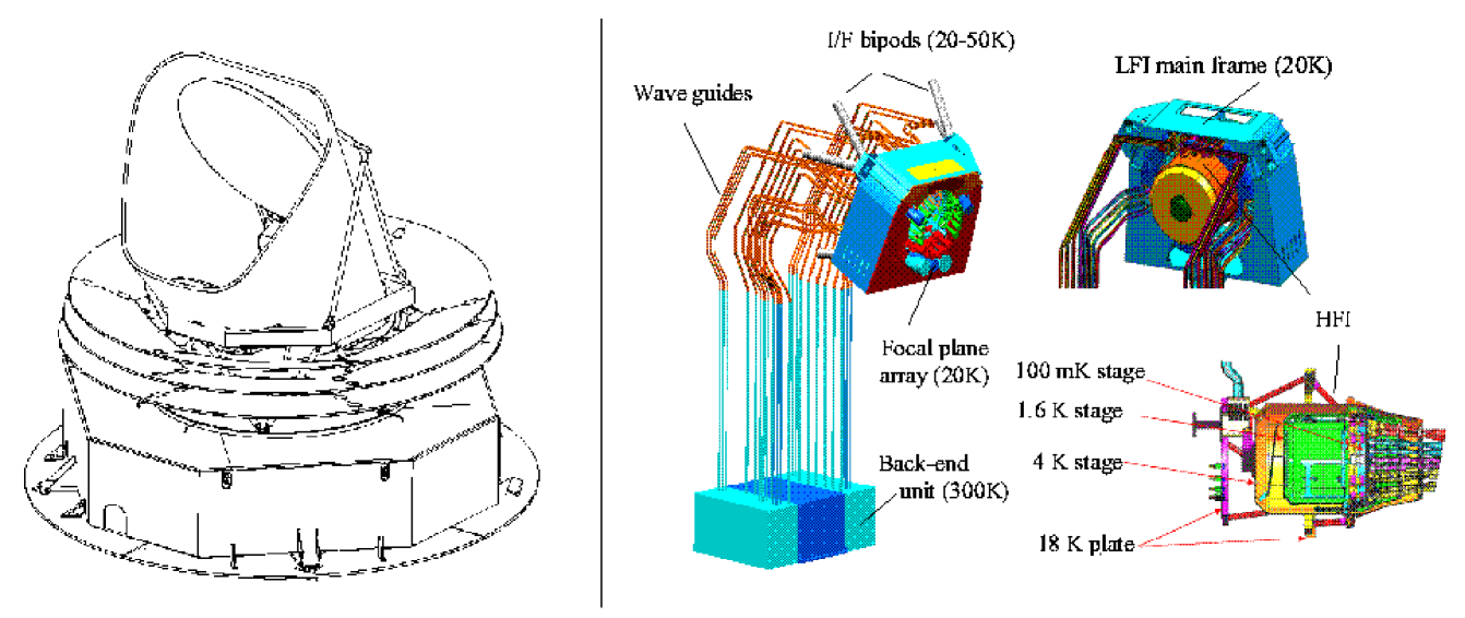
Figure 16: Left: overview of the Planck satellite, showing the primary reflector, the baffle and the three thermal shields (“V-grooves”) used to thermally decouple the cold ($\sim$50 K) telescope enclosure from the warm ($\sim$300 K) service module. The payload design is driven by thermal and radiation (stray-light) requirements. Right: The LFI radiometer array assembly (left) with details of the front-end main frame (upper right) and the HFI instrument (lower right). The two instruments are integrated so that the LFI and HFI horns are located at the focus of the Planck telescope. See text for further details on the two instruments.

The spectral region above 100 GHz is covered by the High Frequency Instrument (HFI), consisting of an array of 48 spider-web bolometers operated at 0.1 K, and distributed in 6 frequency bands from 100 to 850 GHz [120, 351]. Cooling the bolometers to 0.1 K in space is a key driver in the design of the instrument and spacecraft. After the 50-60 K passive cooling and 18 K stage, the HFI cryo-chain uses a mechanical cooler to provide a 4 K stage to HFI, which is also used by LFI to cool the reference loads. The 4 K cooler is designed to minimise microphonic effects, and it operates at a frequency near 40 Hz adjustable in-flight to minimise resonances. Finally, a ³He - ⁴He closed-cycle dilution cooler provides 0.1 K temperature to the bolometers. The focal plane is constituted by an array of back-to-back horns at 4 K with spectral filters placed at $\sim$1.6 K, and a third horn re-images radiation onto the bolometric detector [353]. For the HFI 100, 143 and 217 GHz channels, single-mode propagation is used. For these channels, as well as for LFI, the feed horns use double-profiled corrugated design to optimise telescope illumination and edge taper. At higher frequencies the angular resolution is achieved without diffraction-limited conditions, and multi-moded horns are being employed.

Extraordinary sensitivities ($NEP\sim 1\times 10^{-17}$ W$\times$Hz^-1/2) are achievable with HFI, and have been demonstrated by prototype measurements. Thermal stability requirements are proportionally stringent, at sub-$\mu$K in the 0.1 K stage environment. The use of “spider-web” bolometer technology [123, 124], with silicon nitride micromesh, can provide near-background limited performance (see Sect.4.7). Originally designed as a temperature sensitive instrument only, HFI has been modified to include polarisation sensitivity in a subset of the channels (140–350 GHz) [352]. Eight of the 12 HFI detectors at 143, 217 and 353 GHz use PSBs allowing sensitive polarisation measurements at these frequencies, a factor of 2 less sensitive than for temperature anisotropy. The HFI PSBs are built so that two absorbers made with parallel wires coupled to orthogonal polarisation modes are located in the same cavity and share the same feed horn, filter and optical path.

The Planck payload thermal design is largely driven the extreme thermal requirements (both absolute levels and stability) of the instruments. The spacecraft design allows efficient passive cooling of the payload module (see Fig. 16), as necessary to reach passively $\sim$50 K in the telescope enclosure. To thermally decouple the 300 K service module from the cold focal environment, three intermediate conical V-groove radiators are implemented at temperatures of approximately 140 K, 80 K, and 50 K.

Cooling of both instruments to 20 K is achieved with a closed-cycle hydrogen sorption cryocooler [354, 355, 356]. The cooler operates by thermally cycling a set of compressors filled with metal hydride to absorb and desorb hydrogen gas, which is used as the working fluid in a Joule-Thomson refrigerator. The compressor assembly is attached to a radiator at 280 K in the warm spacecraft, and the hydrogen flow-lines are passively pre-cooled at 50-60 K by the V-groove radiators. The required pressure variations can be obtained by varying by a factor $\sim 2$ the temperature of the compressors. In the complete system six identical compressors are used, each provided with a gas-gap heat switch to optimise their thermal performance. An additional sorbent bed is used to damp pressure fluctuations of the low pressure gas. This principle of operation ensures complete freedom from vibration effects, a unique property of this kind of coolers which is very beneficial to Planck.

Planck requires control of systematic errors at $\mu$K level. The thermal stability at L2 and the thermal design of the payload are such that in general the time scale of thermal drifts will be long compared to the 60 s spin period. Detailed analytical and numerical studies of the main possible sources of systematic effects and their impact on the observations were carried out, including sidelobe pickup of the Galaxy and solar system bodies [128], distorted beam shapes [125, 357, 358], effects induced by temperature instability [135], residual non-white noise components [134, 359], non-idealities in the instruments [130, 360, 361], spacecraft pointing errors and nutation [362] and calibration accuracy [327, 363, 364]. Similarly, the issue of foreground contamination has to be treated at an unprecedented level of detail, and several studies on temperature and polarisation foreground components [145, 365, 366, 367, 368, 369, 370, 371, 372, 373] have been motivated by the perspective of Planck’s survey.

Although Planck’s primary goal is temperature anisotropy, polarisation has taken on increasing importance, even if it does not drive the mission requirements. It is expected that Planck will be able to measure with good accuracy the angular power spectrum of the E-component of CMB polarisation [40], with the consequent improved estimation of cosmological parameters [370, 374]. Based on recent estimates of polarised foreground fluctuations as a function of frequency [63, 367, 375], the minimum fluctuation level should be reached at $\sim 100$ GHz, where the LFI channel has polarisation capability. Foreground polarised fluctuations at 143 GHz are expected to be 1.5 to 2.5 higher, depending on angular scale and location in the sky. The combination of Planck’s polarised channels will help the separation of polarised foregrounds.

Planck is scheduled for an Ariane 5 launch in 2007 together with Herschel (previously called FIRST) from the European spaceport in Kourou (French Guiana). The two satellites will separate soon after launch, and will proceed independently to different orbits around L2. Planck will carry out (at least) two complete surveys, each requiring about 7 months of observing time. While the details of the scanning strategy are still to be finalised, the nominal scanning law consists of hourly manoeuvre of amplitude $2.5^{\prime}$ along the ecliptic plane so as to maintain the spin axis aligned with the sun-satellite direction. The scanning law will be optimised taking advantage of the degree of freedom of moving the spin axis within a $10^{\circ}$ cone centred on the spacecraft-sun line.

While both LFI and HFI, have unprecedented capabilities, it is their combination that gives to Planck the imaging power, the redundancy and the control of systematic effects and foreground emissions needed to achieve the extraordinary scientific goals of the mission. In particular, because systematic effects would in general produce different responses in the two instruments, their frequency overlap at 100 GHz, near the minimum of foreground contamination and with similar angular resolution $\sim 10^{\prime}$, provides Planck with a unique tool to ensure that the final maps are limited only by the instrument sensitivity and unavoidable astrophysical foregrounds.

9 PERSPECTIVES AND CONCLUSIONS

9.1 The Future

The Planck mission is expected to bring the long-lasting effort of measurements of the temperaure power spectrum to its completion. Planck’s precision in the determination of the $C_{\ell}$ may be analogous to that achieved by FIRAS in the measurement of the frequency spectrum [173, 376]. After Planck, it is reasonable to expect a decrease of activity in traditional anisotropy experments, similar to the one we have witnessed in spectrum projects after FIRAS. However, we argue that a lot of exciting CMB observations should happen after Planck, and indeed in some areas Planck will act as a pioneering mission rather than as a conclusive one. Two main research directions can be anticipated: precision measurements of CMB polarisation; and deep imaging at sub-arcminute-scales.

Polarised anisotropy – Though extraordinary, the cosmological information obtainable with temperature anisotropy alone is far less than what could be achieved with a future high-precision full-sky observation of the CMB polarisation. Linear polarisation in the microwave background arises from Thomson scattering of anisotropic radiation at last scattering [379], with an expected amplitude 1% to 10% of the temperature anisotropy. The polarisation depends sensitively on the fluctuations on the LSS, and thus encodes a wealth of cosmological information, some of which is complementary to the temperature anisotropies. Current upper limits (see [316] and references therein) are at a level 10-15 $\mu$K, but the expected signal ($\sim 5$ $\mu$K r.m.s., peaking at multipoles $\ell\sim 1000$) is now in reach of experiments underway: it is likely that statistical detection at sub-degree scales will be achieved before $MAP$ and Planck data become available (see Section 8) . Even the remarkable sensitivity of Planck to $Q$ and $U$ (10–20 $\mu$K per $10^{\prime}$ pixel) will be far from fully extracting the information encoded in the cosmic polarised signal. Planck polarisation data can provide fundamental tests on structure formation from initial adiabatic perturbations and break parameter degeneracy, e.g. between tensor mode amplitude and reionisation optical depth [341]. However, much will be left for further experiments to measure with increasing precision the signature of a background of gravitational waves (tensor modes) as anticipated by inflationary models [52, 380]. A high resolution, high sensitivity polarisation map can be used to discriminate between different inflation models [381] and, in particular, to determine the inflationary energy scale. A broad range of inflation models fit the present data, with a flat geometry ($\Omega_{0}\approx 1$) and nearly scale invariant primordial spectrum ($n_{S}\approx 1$). Polarisation maps will be needed to determine the inflation energy scale, thus probing ultra-high energy physics to levels beyond what can be obtained with any conceivable terrestrial particle accelerator. Even more subtle, but not less interesting, will be to observe the effects of weak gravitational lensing through the distortion of the CMB polarisation on small scales [382].

Significant progress can be anticipated in CMB polarisation experiments from ground and balloon, but a space mission will be needed in the end to avoid atmospheric effects and to map the entire sky – which is needed to extend the measurements to low $\ell$’s and to optimise polarised foreground separation [63, 383]. In fact fluctuations in the synchrotron diffuse component and from extragalactic sources have poorly known and possibly significant impact on the polarised signal. The sensitivity requirements for a full-sky, high-precision polarisation survey are extremely demanding. The expected polarisation amplitude induced by gravitational waves is $\sim 0.1\%$ to 1% of temperature $\Delta T/T$: a high signal-to-noise imaging requires a noise per pixel $\sim$0.05 $\mu$K, i.e. about 300 times better than Planck. This is beyond the foreseeable future, but an intermediate step with sensitivity 0.5 $\mu$K per $10^{\prime}$ resolution element can be approached extrapolating existing technology. Multi-frequency observations, possibly with matching FWHM, would be needed for foreground separation. It is difficult to anticipate which systematic effects could represent limiting factors at sub-$\mu$K levels; it is likely that thermal stability at the cryogenic temperatures needed by the ultra-high sensitivity detectors (either radiometers or bolometers) will be a major challenge; also, a multi-channel off-axis instrument, pushed at extreme sensitivities, would place critical requirements for ultra-low cross-polarisation.

Fine scale CMB – On angular scales $\sim 1^{\prime}$ and below the CMB is influenced by interaction with intervening ionised material (see Sect. 2.4). The CMB passed through the cosmic “dark ages”, before star and quasar formation, from which direct observation is extremely difficult to obtain. The study of arcmin scale features in the CMB may well turn out to be the only, or one of the most powerful, technique to gather observational evidence from the very early processes of structure formation. Using the CMB as a high redshift backlight, deep arcminute CMB imaging can probe the early history of galaxy clusters and their gradual acceleration as they fell in their potential wells. In addition, CMB fine scale observations can provide images of the largest structures in the universe as they started to dissipate the heat of their gravitational collapse. Planck will open up this field, but its $>5^{\prime}$ angular resolution is not sufficient to fully cover this promising area of CMB studies. Furthermore, accurate S-Z measurements can be made to very high redshifts [384], all the way back to the cluster formation era [343]. A future sky survey of clusters velocities based on their S-Z features throughout the entire Hubble volume could, in principle, map the evolution of velocity fields over much of the history of the universe.

The S-Z effect from clusters is by far the dominant secondary source (see Sect. 2.4). Once this will be well identified and mapped, sky regions free from S-Z and other local foregrounds could be searched at $\sim 1^{\prime}$ scales for fainter secondary signatures, such as those from gravitational collapse of large scale ($\sim 100$ Mpc) structures, bulk motion of plasma (the “Ostriker-Vishniac effect”), effects of the evolution of gravitational potentials on CMB photons (the “integrated Sachs-Wolfe effect” and the “Rees-Sciama effect”), lensing-induced signatures from clusters [385], signature of local ionisation events [386], and details of the ionisation history of the universe.

It is easy to expect that the $MAP$ and (especially) Planck surveys will trigger new observations in selected sky areas searching for detailed, physically interesting features. New instruments and observing strategies will be developed for the purpose. At wavelengths $\lambda\approx 1~{}$mm, a $\lesssim 1^{\prime}$ resolution translates in a telescope aperture typically $D\sim 10$ m. The brightest clusters give a S-Z thermal component $\sim 1$ mK, while the kinetic effects is expected to be $\sim 10$ times lower. Signatures such as filaments from in-falling clusters are expected at $\sim$10 $\mu$K level. Current bolometric or HEMT-based instruments (either filled aperture arrays or interferometers) are able to approach sub-$\mu$K sensitivity in very localised areas. High precision fine-scale CMB imaging would call for very wide frequency coverage, with ancillary monitoring at low frequency ($<5$ GHz) and high frequency ($>5$ THz) to safely remove unrelated foregrounds as well as backgrounds (such as primary CMB anisotropy, a source of confusion in this context!). These observations can be expected to progress for several years with ground-based instrumentation. Eventually, an arcminute-scale, full-sky survey to map the evolution of the large scale velocity field will only be possible with a space programme, currently out of reach.

9.2 Conclusions

Observations of the CMB anisotropy can be considered at present as the most powerful method to obtain high quality data on the early universe. We have reviewed the great effort that is being carried out by sub-orbital projects after the $COBE$-DMR discovery. In spite of the major experimental challanges, a coherent picture is emerging. Both balloon-borne and ground-based experiments independently demonstrate the acoustic pattern of the angular power spectrum showing the first three peaks, and both provide a determination $\sim 10\%$ accuracy of the angular scale of first peak consistent with a flat geometry, $\Omega_{0}\approx 1$. This is a truly remarkable achievement. However, it is only a foretaste of the precise (percent-level) determination of several cosmological parameters attainable by the forthcoming generations of experiments, culminating with the Planck space mission. Beyond Planck, it is likely that CMB observations will concentrate on precise polarisation measurements and deep sub-arcmin imaging searching for secondary anisotropies.

Precision measurements of the CMB temperature and polarisation fluctuations are able to shed light on very high energy phenomena occurring in the primordial cosmic environment. Cosmologists need to look more and more towards particle physics to interpret the physical processes probed by CMB data. On the other hand, exploiting the natural laboratory of the early universe to study ultra-high energy scales is of great interest for particle physics. The enormous data sets expected from the planned and future CMB missions are likely to attract the interest of a wider scientific community.

- [1] \BYPenzias A. & Wilson R. \INApJ1421965419
- [2] \BYGamow G. \INPhys. Rev.741948506
- [3] \BYAlpher R.A. & Herman R.C. \INNature1621948774
- [4] \BYWalker P.N. \INApJ376199151
- [5] \BYHubble E.P. \INProc. Natl. Acad. Sci. U.S.151929169
- [6] \BYDanese L. & De Zotti G. \INIl Nuovo Cimento71977277
- [7] \BYBurigana C. et al. \INA& A246199149
- [8] \BYFixsen D.J. et al. \INApJ4731996576
- [9] \BYBersanelli M. et al. \INApJ4241994517
- [10] \BYDe Amici G. et al. \INApJ3811991341
- [11] \BYBensadoun M. et al. \INApJ40919931
- [12] \BYSmoot G.F. et al. \INApJL3171987L45
- [13] \BYSironi G. et al. \INApJ3781991550
- [14] \BYSalvaterra R. & Burigana C \INMNRAS2002in press – astro-ph/0203294
- [15] \BYSmoot G.F. et al. \INApJL3961982L1
- [16] \BYHu W. & Dodelson S. \INARA&A402002171
- [17] \BYWhite M., Scott D. & Silk J. \INARA&A321994319
- [18] \BYSmoot G.F., Gorestein M.V., & Muller R.A. \INPhys. Rev. Lett391977898
- [19] \BYWald R.M. \INGeneral Relativity1994The University of Chicago Press, Chicago
- [20] \BYDe Bernardis P. et al. \INApJ2001submitted
- [21] \BYHanany S. et al. \INApJL5452000L5
- [22] \BYSilk J. \INNature21519671155
- [23] \BYSilk J. \INApJ1511968459
- [24] \BYPeebles P.J.E. & Yu J.T. \INApJ1621970815
- [25] \BYLinde A. \INParticle Physics and Cosmology1990Harwood Academic, Chur, Switzerland
- [26] \BYBond J.R. \INLes Houches Lect., R. Schaefer Ed., Elsevier Science Publishers, The Nederlands1996
- [27] \BYColes P. & Lucchin F. \INCosmology - Origin and Evolution of Cosmic Structure1995Wiley
- [28] \BYHu W. & Sugiyama N. \INApJ4441995489
- [29] \BYSeljak U. \INApJL4351994L87
- [30] \BYVittorio N., & Silk J. \INApJ285198439
- [31] \BYBond J.R. & Efstathuou G. \INApJL2851984L45
- [32] \BYAllen B. et al. \INPhy. Rev. D7919972624
- [33] \BYFerreira P. \INPhy. Rev. Lett7419953522
- [34] \BYTurok N. \INApJL47319965
- [35] \BYGangui A. & Jerôme M. \INMNRAS3132000323
- [36] \BYSachs R.K. & Wolfe A.M. \INApJ147196773
- [37] \BYRees M.J. & Sciama D.W. \INNature5171968611
- [38] \BYBond J.R. & Efstathuou G. \INMNRAS2661987655
- [39] \BYSmoot G.F. \INProceedings of the 26th Moriond Astrophy. Meeting19973
- [40] \BYHu W. & White M. \INApJ4791997568
- [41] \BYZaldarriaga M. & Seljak U. \INPhys. Rev. D591999123507
- [42] \BYSunyaev R.A. & Zeldovich Y. \INAstroph. Sp. Sci.719703
- [43] \BYRephaeli Y. \INARA&A331995541
- [44] \BYSunyaev R.A. & Zeldovich Y. \INMNRAS1901980413
- [45] \BYRephaeli Y. et al. \INApJ3801991344
- [46] \BYJungman G. et al. \INPhys. Rev. Lett.7619961007
- [47] \BYHu W. et al. \INPhys. Rev. D5219955498
- [48] \BYBurles S & Tytler D. \INApJ4991998699
- [49] \BYTegmark M., Zaldarriaga M. & Hamilton A.J.S. \INPhysRevD2002in press
- [50] \BYKaiser N. \INMNRAS20219831169
- [51] \BYKamionkowski M. et al. \INPhys. Rev. D5519977368
- [52] \BYSeljak U. & Zaldarriaga M. \INPhys. Rev. Lett.7819972054
- [53] \BYZaldarriaga M., Seljak U. & Spergel D. \INApJ48819971
- [54] \BYSmoot G.F. \INMicrowave Foregrounds, ASP Conference Series181199961
- [55] \BYHaslam C.G.T. et al. \INA& A SS4719821
- [56] \BYReich P. & Reich \INA&ASS631986106
- [57] \BYJonas J.L., Baart E.E. & Nicolson G.D. \INMNRAS2971998977
- [58] \BYDavies R.D. et al. \INMNRAS2781996925
- [59] \BYPlatania P. et al. \INApJ5051998473
- [60] \BYSmoot G.F. et al. \INApJL2911985L23
- [61] \BYTegmark M. & Efstathiou G. \INMNRAS28119961297
- [62] \BYLanseby A. \INProceedings of the 26th Moriond Astrophy. Meeting1997453
- [63] \BYBaccigalupi C. et al. \INA& A37220018
- [64] \BYPaladini R. \INA & A(2002)in press
- [65] \BYKogut A. et al. \INApJ46019961
- [66] \BYLeitch E.M. et al. \INApJL4861997L23
- [67] \BYDe Oliveira-Costa, A. et al. \INApJL4821997L17
- [68] \BYGaustad J.E., Mc Cullough P.R. & Van Buren D. \INPASP1081996351
- [69] \BYDraine B.T. & Lazarian A. \INApJL4941998L19
- [70] \BYSchlegel D.J., Finkbeiner D.P. & Davis M. \INApJ5001998525
- [71] \BYGautier T.N.I. et al. \INAJ10319921313
- [72] \BYFranceschini A. et al. \INApJ344198935
- [73] \BYToffolatti L. et al. \INMNRAS2971998117
- [74] \BYDanese L. et al. \INApJL3181987L15
- [75] \BYFranceschini A. et al. \INThe Far Infrared and Submillimitre UniverseESA SP-4011997159
- [76] \BYDe Zotti G. et al. \INProc. “3K Cosmology from Space”, Rome, I1998astro-ph/9902103
- [77] \BYBond J.R. et al. \INPhys. Rev. Lett6619912179
- [78] \BYReadhead A.C.S., & Lawrence C.R. \INAnnual review of astronomy and astrophysics301992653
- [79] \BYKnox L. \INPhys. Rev. D4819953502
- [80] \BYDanese L. & Partridge B. \INApJ3421989604
- [81] \BYDavies R.D. et al. \INMNRAS2581992605-615
- [82] \BYLasenby A.N. et al. \INLecture Notes in Physics429199491
- [83] \BYMeinhold P. and Lubin P. \INApJL3701991L1
- [84] \BYMeinhold P. et al. \INApJ406199312
- [85] \BYBersanelli M. et al. \INApJ4241994517
- [86] \BYKogut A. et al. \INApJ40119921
- [87] \BYBennett C.L. et al. \INApJ4361994423
- [88] \BYDe Pater I. \INARA&A281990347
- [89] \BYKogut A. et al. \INApJ4701996653
- [90] \BYMasi S. et al. \INApJ2002submitted
- [91] \BYCappellini B. et al. \INA& A2002submitted
- [92] \BYBennett C.L. et al. \INApJ3911992466
- [93] \BYBersanelli M., Muciaccia P.F., Natoli P., Vittorio P., & Mandolesi N. \INA& A Suppl12219961
- [94] \BYSmoot G. et al. \INApJ3601990685
- [95] \BYPage L.A., Cheng E.S., and Meyer S.S. \INApJL355(1)1990L1-L4
- [96] \BYMeyer S.S., Cheng E.S., and Page L.A. \INApJL371(1)1991L7-L9
- [97] \BYKraus J.D. \INRadio Astronomy1966McGraw-Hill, New York
- [98] \BYJarosik N. \INIEEE Trans. Microwave Theory Tech.MIT-441996193
- [99] \BYDicke R.H. \INRev. Sci. Instruments171946269
- [100] \BYFaris J.J. \INJ. Res. Nat. Bur. Stand.Sect 71C1967153
- [101] \BYPartridge R.B. \IN3K: The Cosmic Microwave Background Radiation1995Cambridge Astrophysics Seiries
- [102] \BYHaslam C.G.T. et al. \INA& A Suppl.131974359
- [103] \BYHaslam C.G.T. et al. \INA&A1001981209
- [104] \BYStaggs S.T., Jarosik N.C., Meyer S.S., & Wilkinson D.T. \INApJ47319961
- [105] \BYRead-Predmore C. et al. \INIEEE Trans. Microwave Theory & Technique33198544
- [106] \BYNatoli P. et al. \IN“Cosmology and Particle Physics”, Proc. of the CAPP, 2000 Conference, Verbier, Switzerland, eds. J. Garcia-Bellido, R. Durrer and M. Shaposhnikov (AIP, 2001)5552001324-327
- [107] \BYMakunda B.D. \INIEEE Trans. On Electr. Devices, ED-34719871429
- [108] \BYWeinreb S. \INIEEE Trans. Microwave Theory & TechniquesMIT-2819801041
- [109] \BYPospieszalski M.W. et al. \INProc. 1994 IEEE MTT-S Int. Microwave Symp.19941345-1346
- [110] \BYPospieszalski M.W. et al. \INIEEE MTT-SW DigestTH2B-219951121
- [111] \BYPospieszalski M.W. \INProceedings of the workshop Microwave Background Anisotropies; Edition Frontieres, F. Bouchet et al. Eds.199723
- [112] \BYMiller A.D. et al. \INApJL5241999L1
- [113] \BYTucker J.R. \INIEEE Journal of Quantum ElectronicsQE-1519791234
- [114] \BYKerr A.R., & Pan S.K. \INInt. J. Infrared & Millimeter Waves11(10)19901169
- [115] \BYXiaolei Z. \INIEEE Trans. Microwave Theory & Techniques4119931263
- [116] \BYToral M.A. et al. \INIEE Trans. Ant. & Propagation371989171
- [117] \BYGentili G.G., Nesti R., Pelosi G. & Natale V. \INElectronics Letters362000486
- [118] \BYVilla F. et al. \INExperimental Astronomy2002in preparation
- [119] \BYBersanelli M. et al. \INExperimental Astronomy8(3)1998231
- [120] \BYLamarre J.-M. \INProceedings of the workshop Microwave Background Anisotropies, Les Arches, March 1996 – Edition Frontieres, F. Bouchet et al. Eds.199731
- [121] \BYMather J.C. \INAppl. Optics21(6)19821125
- [122] \BYLamarre J-M. \INAppl. Optics251986870
- [123] \BYBock J.J., et al. \INProceedings of “Submillimeter and Far-Infrared Space Instrumentation”; 30-th ESALAB Symposium 24-46 Spetember 1996, ESTEC, Noordwijk, The Netherlands1996
- [124] \BYLange A.E. et al. \INProceedings of “Submillimeter and Far-Infrared Space Instrumentation”; 30-th ESALAB Symposium 24-46 Spetember 1996, ESTEC, Noordwijk, The Netherlands1996
- [125] \BYBurigana C. et al. \INA& A Suppl1301998551-560
- [126] \BYVilla F., Valenziano L., Burigana C., Mandolesi N., Bersanelli M. \INProceedings of the XXIIIrd Moriond Symposium on “Fundamental Parameters in Cosmology” Les Arcs, Savoie, France, January 1998. Edited by J.Tran Than Van, Y.Giraud-Heraud, F.Bouchet, T.Damour, Y.Mellier – Edition Frontieres.1998
- [127] \BYMandolesi N. et al. \INA&A Suppl1452000323
- [128] \BYBurigana C. et al. \INA& A3732001345
- [129] \BYMaino D. \INSISSA Ph.D. Thesis1999
- [130] \BYSeiffert M. et al. \INA& A accepted2002astro-ph/0206093
- [131] \BYJanssen M., et al. \INTech. rep. PSI-96-01, FIRE-96-011996astro-ph/9602009
- [132] \BYPrunet S. et al. \IN2000astro-ph/0006052
- [133] \BYBurigana C. et al. \INITeSRE Internal Report1997198/97
- [134] \BYMaino D. et al. \INA& A Suppl1401999383
- [135] \BYMennella A. et al. \INA&A3842002736-742
- [136] \BYDe Bernardis P. et al. \INNew Astronomy Reviews431999289-296
- [137] \BYDe Bernardis P. et al. \INNature4042000955
- [138] \BYBurigana C. et al. \INAstroph. Lett. Comm.372000253
- [139] \BYDoré O. et al. \INsubmitted to A&A2002astro-ph/0101112
- [140] \BYNatoli P. et al. \INA&A38320021100
- [141] \BYPress et al. \INNumerical Recipies in Fortran 90, Cambridge University Press, Cambridge1996
- [142] \BYNatoli P. et al. \INA&A3722001346
- [143] \BYWiener N. \INExtrapolation and Smoothing of Stationary Time Series1949New York, Wiley
- [144] \BYSkilling J. \INMaximum Entropy and Bayesian Methods1989Kluwer, 45
- [145] \BYHobson M.P. et al. \INMNRAS30019981
- [146] \BYBunn E.F. et al. \INApJL4321994L75
- [147] \BYTegmark M. et al. \INApJL4741997L77-80
- [148] \BYBaccigalupi C. et al. \INMNRAS318(3)2000769
- [149] \BYMaino D. et al. \INMNRAS334(1)200253
- [150] \BYOh S.P., Spergel D.N. & Hinshaw G. \INApJ5101999551
- [151] \BYGórski K.M. et al. \INApJL4301994L85
- [152] \BYGórski K.M. et al. \INApJL4301994L89
- [153] \BYGórski K.M. \INProceedings of the XVIth Moriond Astrophysics Meeting “Microwave Background Anisotropies”, Les Arcs, Savoie, France, March 16th-23rd 1996. Edited by F.R. Bouchet, R.Gispert, B. Guiderdoni & J. Tran Thanh Van199677
- [154] \BYBorrill J. \INProceedings of the 5th European SGI/Cray MPP Workshop1999astro-ph/9911389
- [155] \BYBalbi A. et al. \INApJ545L20005
- [156] \BYWandelt B.D. & Hansen F.K. \INPhys. Rev. D2002in press
- [157] \BYHivon E. et al. \INApJ56720022
- [158] \BYNetterfield C.B. et al. \INApJ5712002604
- [159] \BYBalbi A. et al. \INsubmitted to A&A2002astro-ph/0203159
- [160] \BYSzapudi I., Prunet S. & Colombi S. \INApJL5612001L11
- [161] \BYKashlinsky A., Hernandez-Montegudo C. & Atrio-Barandela F. \INApJL5572001L1
- [162] \BYBennett C.L. et al. \INApJL3961992L7
- [163] \BYGanga K. et al. \INApJL391(2)1993L49-L52
- [164] \BYLineweaver C.H. et al. \INApJ4481995482
- [165] \BYBennett C.L. et al. \INApJL4641996L1
- [166] \BYGorski K.M. \INApJL4641996L11
- [167] \BYHinshaw G. et al. \INApJL4641996L17
- [168] \BYHinshaw G.et al. \INApJL4641996L25
- [169] \BYWright E.L., et al. \INApJL4641996L21
- [170] \BYKogut A. et al. \INApJL4641996L29
- [171] \BYBanday A.J.et al. \INApJL4681996L85
- [172] \BYBanday A.J.et al. \INApJ4751997393
- [173] \BYFixsen D.J. et al. \INApJ4861997623
- [174] \BYFixsen D.J. et al. \INApJ470199663
- [175] \BYLay O.P., & Halverston N.W. \INApJ5432000787
- [176] \BYGaier T. et al. \INApJL3981992L1
- [177] \BYSchuster J. et al. \INApJL4121993L47
- [178] \BYGunderson J.O. et al. \INApJL4431995L57-L60
- [179] \BYTucker G.S., Griffin G.S., Nguyen H.T., & Peterson, J.B. \INApJL4191993L45
- [180] \BYPeterson J.B. et al. \INAstroph. Lett. Comm.321995269
- [181] \BYTucker G.S.et al. \INRev. Sci. Instr.651994301
- [182] \BYFemenia B. et al. \INApJ4981998117
- [183] \BYPiccirillo L. \INRev. Sci. Instr.6219911293
- [184] \BYPiccirillo L., & Calisse P. \INApJL4751993L77
- [185] \BYHancock S. et al. \INAstroph. Lett and Comm.321995201
- [186] \BYGutierrez C. M. et al. \INApJ529(1)200047-55
- [187] \BYRomeo G. et al. \INApJL5482001L1
- [188] \BYLasenby A., and Davies R. \INMNRAS20319831137
- [189] \BYWatson R.A. et al. \INNature3571992660-664
- [190] \BYDavies R.D. et al. \INAstroph. Lett. & Comm.321995183
- [191] \BYRebolo R. et al. \INAstroph. Lett and Comm.321995211
- [192] \BYGutierrez C.M. et al. \INApJ529200047
- [193] \BYDragovan M. et al. \INApJL4271994L67
- [194] \BYRuhl J.E. et al. \INApJL4531995L1
- [195] \BYPlatt S. R. et al. \INApJL4751997L1
- [196] \BYRuhl J.E., & Dragovan M. \INLow temperature detectors for Neutrinos and dark matter, ed. N.e. Booth and G.L. Salmon, Editioned Frontieres11992161
- [197] \BYDragovan M. et al. \INAAS Bull.251993927
- [198] \BYKovac J. et al. \INProc. American Astronomical Society Meeting1911997112.04
- [199] \BYCoble K. et al. \INApJL5191999L5
- [200] \BYGundersen J. O. et al. \INApJL4431995L57
- [201] \BYSchlegel D.J., Finkbeiner D.P., and Davis M. \INApJ5001998525
- [202] \BYHaslam C.G. et al. \INA& A Suppl4719821
- [203] \BYPeterson J.B. et al. \INApJL532, 22000L83-L86
- [204] \BYGriffin G. et al. \INProc. American Astronomical Society Meeting192199858.03
- [205] \BYBeichman C.A. et al. \INIRAS Explanatory Supplement, Scientific and Technical Information Division National Aeronautics and Space Administration 1988 Washington, DC1988
- [206] \BYRomer A.K. et al. \INProc. American Astronomical Society Meeting194199958.03
- [207] \BYWollack E. J., Jarosik N.C., Netterfield C.B., Page L.A., & Wilkinson D. \INApJ4191993(L49)
- [208] \BYWollack E.J.n et al. \INApJ4761997(440)
- [209] \BYde Oliveira-Costa et al. \INApJL4821997L17
- [210] \BYTorbet E. et al. \INApJL5211999L79
- [211] \BYMiller A.D. et al. \INApJ SS1402002115
- [212] \BYUlich, B.L. \INAstron. J.8619811619
- [213] \BYGriffin M.J. et al. \INIcarus65244
- [214] \BYGriffin M.J., & Orton G.S. \INIcarus1051993537
- [215] \BYGregory P.C., Vavasour J.D., Scott W.K., & Condon J.J. \INThe PNM Catalog of Radio Sources. NRAO, Charlottesville1993
- [216] \BYGriffith M.R., & Wright A.E. \INParkes-MIT-NRAO (PMN) Surveys, VizieR On-line Data Catalog: VIII/271994
- [217] \BYScott P.F. et al. \INApJL4611996L1
- [218] \BYO’Sullivan C. \INIrish Astronomical Journal23(2)1996161
- [219] \BYBaker J.C. \INMonthly Notices of the Royal Astronomical Society308(4)19991173-1178
- [220] \BYGull S.F. \INMaximum Entropy and Bayesian Methods, J.Skilling (ed), Kluwer Academic Publishers, Dordtrecht198953
- [221] \BYFomalont E.B., Kellerman K.I., Wall J.V., & Weistrop D. \INScience225198423
- [222] \BYKnoke J.E., Partridge R.B., Ratner M.I., & Shapiro I.I. \INApJ2841984479
- [223] \BYMartin H.M., & Partridge B. \INApJ3241988794
- [224] \BYPartridge B. et al. \INNature3311988146
- [225] \BYFomalont E.B., Partridge R.B., Lowenthal J.D., & Windhorst R.A. \INApJ40419938
- [226] \BYPartridge R.B., Richards E.A., Fomalont E.B., Kellerman K.I., & Windhorst R.A. \INApJ483199738
- [227] \BYWindhorst R.A., et al. \INNature3751995471
- [228] \BYKellerman K.I. et al. \INHighligts of Astron.71986367
- [229] \BYSubrahmanyan R. et al. \INMNRAS2631993416
- [230] \BYSubrahmanyan R. et al. \INMNRASaccepted2000
- [231] \BYReadhead A.C.S. et al. \INApJ3461989566
- [232] \BYMyers S.T., Readhead A.C.S., & Lawrence C.R. \INApJ40519938
- [233] \BYLeitch E.M. et al. \INApJ532200037
- [234] \BYChurch S.E. et al. \INApJ1997484523
- [235] \BYWilbanks T.M., Ade P.A.R., Fisher M.L., Holzapfel W.L., & Lange A.E. \INApJL1994427L75
- [236] \BYHolzapfel W. L. et al. \INApJ199747917
- [237] \BYBecker R.H., White R.L., & Edwards A.L. \INApJS1991751
- [238] \BYMelhuish S.J. et al. \INMNRAS305(2)1999399-408
- [239] \BYDicker S.R. et al. \INMNRAS309(3)1999750-760
- [240] \BYHancock S. et al. \INMNRAS2981997505
- [241] \BYLasenby A.N. \INMicrowave Background Anisotropies1996Bouchet F., Tran Thanh Van J., eds, 31st Recontre de Moriond, Editions Frontiers, Gif-sur-Yvette - astro-ph/9611214
- [242] \BYDavies R. D., & Wilkinson A. \INFundamental Parameters in Cosmology1998Bouchet F., Tran Thanh Van J., eds, 33rd Recontre de Moriond, Editions Frontiers, Gif-sur-Yvette
- [243] \BYTerasranta H. et al. \INA& A Suppl941992121
- [244] \BYHalverson N.W. et al. \INApJ2001submitted
- [245] \BYPospieszalski M.W. \INProc. of 23rd European Microwave Conf.6199373-79
- [246] \BYLeitch E.M. et al. \INApJ568200228
- [247] \BYPadin S. et al. \INIEEE Trans. Antennas Propagat482000836-838
- [248] \BYCartwright J. K. et al. \INProc. American Astronomical Society meetingJan. 9, 2001
- [249] \BYPadin S. et al. \INApJL)5492001L1-L5
- [250] \BYPearson J.T. et al. \INSubmitted to ApJ2002astro-ph/0205388
- [251] \BYSievers J.L. et al. \INSubmitted to ApJ2002astro-ph/0205387
- [252] \BYMyers S.T. et al. \INSubmitted to ApJ2002astro-ph/0205385
- [253] \BYBond J.R. et al. \INSubmitted to ApJ2002astro-ph/0205386
- [254] \BYWeiss R. \INAnnual Rev. Astr. Astrophis.181980489
- [255] \BYStaren J. et al. \INApJ539200052
- [256] \BYLee A.T. et al. \INApJL5612001L1-L6
- [257] \BYPage L.A., et al. \INApplied Optics33(1)199411-23
- [258] \BYPage L. et al. \INAstroph. Lett. and Comm.321995239
- [259] \BYGanga K., Page L., Cheng E., & Meyer S. \INApJL4321994L15
- [260] \BYDe Bernardis P et al. \INApJL4331994L1
- [261] \BYPalumbo P. et al. \INCryogenics3419941001
- [262] \BYMasi S. et al. \INApJL4631996L47
- [263] \BYHalpern M, Gush M.P., Shinkoda I., Tucker G.S., & Towlson W. \INAstroph. Lett & Comm.321995283
- [264] \BYTucker G.S., Gush H.P., Halpern M., & Towlson W. \INProceedings of the workshop Microwave Background Anisotropies, Les Arches, March 1996, Edition Frontieres, F. Bouchet et al. Eds1997167
- [265] \BYTucker G.S. et al. \INApJL475199773
- [266] \BYGush H.P., Halpern M., & Wishnow E. \INPhys. Rev. Lett.651990537
- [267] \BYGush H.P., & Halpern M. \INRev. Sci. Inst.6319923249
- [268] \BYFisher M.L. et al. \INApJ3881992242
- [269] \BYAslop D.C. et al. \INApJ3951992317
- [270] \BYGundersen J.O. et al. \INApJL4131993L1
- [271] \BYMeinhold P.et al. \INApJL4091993L1
- [272] \BYClapp A.C. et al. \INApJL4331994L57
- [273] \BYDevlin M.J. et al. \INApJL4301994L1
- [274] \BYTanaka S. et al. \INApJL4681996L81
- [275] \BYMeinhold P. et al. \INApJ406199312
- [276] \BYLim M.A. et al. \INApJL4691996L69
- [277] \BYCheng E.S. et al. \INApJL4221994L37
- [278] \BYCheng E.S. et al. \INApJL4561996L71
- [279] \BYInman C.A. et al. \INApJL4781997L1
- [280] \BYKnox L., Bond J., Jaffe A., Segal M., & Carbonneau D. \INPhys Rev. D581998id 083004
- [281] \BYCheng E.S. et al. \INApJL4881997L59
- [282] \BYKowitt M.S. et al. \INApJ482199717
- [283] \BYPospieszalski M.W. \INProc. IEEE Microwave Theory Tech.3719891340
- [284] \BYDe Oliveira-Costa A. et al. \INApJL5091998L9
- [285] \BYBaars J.W.M., Genzel R., Pauliny-Toth, I.I.K., & Witzel A. \INA& A61197799
- [286] \BYChini R., Kreysa E., Mezger P. G., & Gem. und H.P. \INA& A1371984117
- [287] \BYMezger P. G., Tu-s R.J., Chini R., Kreysa E., & Gem. und H.P. \INA& A1671986145
- [288] \BYDevlin M.J. et al. \INApJL5091998L69
- [289] \BYHerbig T. et al. \INApJL5091998L73
- [290] \BYMason B.S., Leitch E.M., Myers S.T., Cartwright J.K., & Readhead A.C.S. \INAJ118(6)19992908
- [291] \BYXu Y. et al. \INPhys.Rev. D652002083002
- [292] \BYPark C.G. et al. \INApJ556(2)2001582
- [293] \BYMauskopf P. et al. \INApJL5362000L59
- [294] \BYMelchiorri A. et al. \INApJL5362000L63
- [295] \BYMasi S. et al. \INCryogenics381998319
- [296] \BYMasi S. et al. \INCryogenics391999217
- [297] \BYNetterfield C.B. et al. \INApJ5712002604
- [298] \BYLange A.E. et al. \INPhys. Rev. D632001042001
- [299] \BYFreedman W.L. et al. \INApJ553200147
- [300] \BYLee A.T. et al. \INProc. “3K Cosmology from Space”, Rome, I1998astro-ph/9903249
- [301] \BYStompor R. et al. \INApJL5612001L7
- [302] \BYWu J.H.P. et al. \INPhys.Rev.Lett.872001251303
- [303] \BYWang X., Tegmark M. & Zaldarriaga M. \INPhys.Rev.D652002123001
- [304] \BYBenoit A. et al. \INAstroparticle Physics17(2)2002101-124
- [305] \BYKowitt M.S. et al. \INAstroph. Lett & Comm.321995273
- [306] \BYScott F.S. et al. \IN2002astro-ph/0205380
- [307] \BYKesteven M. et al. \INAstropysical Polarised Backgrounds – AIP Conference Proceedings6092002156
- [308] \BYLo K.Y. et al. \INIAU Symposium 201 – New Cosmological Data and the Values of the Fundamental Parameters, eds. Lasemby, A. and Wilkinson, A.2000
- [309] \BYKuo C.L. et al. \INProc. AAS 200th meeting, Albuquerque, NM, June 200220026
- [310] \BYParijskij Y., Chepurnov A., & Bursov N. \INMicrowave Background Anisotropies1997117
- [311] \BYCaderni N. \INPhys. Rev. D.1719781901
- [312] \BYNanos G.P. \INApJ2321979241
- [313] \BYLubin P., & Smoot G. \INApJ24519811
- [314] \BYWollack E. et al. \INApJ4761997440
- [315] \BYNetterfield C.B. et al. \INApJ474199747
- [316] \BYHedman M. et al. \INApJ Lett.5482001111
- [317] \BYSubrahmanyan R. et al. \INMNRAS3152001808
- [318] \BYKeating B.G. et al. \INApJL5602001L1
- [319] \BYKovac J et al. \INApJ - submitted2002astro-ph/0209478
- [320] \BYCortiglioni E. et al. \INAIP Conference Proceedings504200091
- [321] \BYCarretti E. et al. \INNew Astronomy62001173
- [322] \BYCarretti E. et al. \INAIP Conference Proceedings6092002109
- [323] \BYZannoni M. et al. \INAIP Conference Proceedings6092002115
- [324] \BYMasi S. et al. \INAIP Conference Proceedings6092002122
- [325] \BYPiccirillo L. et al. \INAIP Conference Proceedings6092002159
- [326] \BYMandolesi N., Smoot G.F., & Bersanelli M. \INProceedings of Workshop on Present and Future of the Cosmic Microwave Background, J.L.Sanz, E.Martinez-Gonzales, L.Cayon Eds., Springer–Verlag1994228
- [327] \BYBersanelli M., Mandolesi N., & Smoot G.F. \INMem. S.A.It.66-1199539
- [328] \BYBersanelli M. et al. \INAstroph. Lett & Comm.3319
- [329] \BYJanssen M. A., & Lawrence C.R. \INAstroph Lett and Comm321995289
- [330] \BYDanese L., Toffolatti L., Franceschini A., Bersanelli M., & Mandolesi N. \INAstrophysical Lett & Comm.331996257
- [331] \BYLange A. \INProceedings of the workshop Microwave Background Anisotropies, Les Arches, March 1996, Edition Frontieres, F. Bouchet et al. Eds1997173
- [332] \BYTauber J. \INProceedings of the workshop Microwave Background Anisotropies, Les Arches, March 1996, Edition Frontieres, F. Bouchet et al. Eds199757
- [333] \BYPospieszalski M.W. \INProc. IEEE Microwave Theory Tech.MTT-319921369
- [334] \BYPospieszalski M.W.& Wollak E. \INProceedings of the European GaAs Application Symposium - Paris (GAAS2000)2000
- [335] \BYJarosik N. \INProc. European GaAs Appl. Symp., Paris (F)2000
- [336] \BYWright E., Hinshaw G. & Bennett C. \INTech. Report UCLA-ASTRO-ELW-95-041995astro-ph/9510102
- [337] \BYHinshaw G. \INProceedings of the MPA/ESO/MPE Workshop held at Garching, Germany, 31 July-4 August, 2000. Edited by A. J. Banday, S. Zaroubi, and M. Bartelmann. Heidelberg: Springer-Verlag2001447 - astro-ph/0011555
- [338] \BYDraine B.T., &Lazarian A. \INReview for the Sloan Summit on Microwave Foregrounds, ed. A. de Oliveira-Costa and M. Tegmark1999astro-ph/9902356
- [339] \BYTauber J. \INProceedings of the XXIIIrd Moriond Symposium on “Fundamental Parameters in Cosmology” Les Arcs, Savoie, France, January 1998. Edited by J.Tran Than Van, Y.Giraud-Heraud, F.Bouchet, T.Damour, Y.Mellier – Edition Frontieres.1998
- [340] \BYBond J.R., Efstathiou G., & Tegmark M. \INMNRAS2911997L33
- [341] \BYEfstathiou G. \INMNRAS3322002193
- [342] \BYMartinez-Gonzalez E. \INAstr. Letter and Communications372000335
- [343] \BYAghanim N., de Luca A., Bouchet F.R., Gispert R., & Puget J.L. \INA& A32519979
- [344] \BYHaehnelt M.G. & Tegmark M. \INMNRAS2791996545
- [345] \BYDa Silva A.C., et al. \INMNRAS317(1)200037-44
- [346] \BYPasian F., Mandolesi N. & Bersanelli M. \INS.A.It. AstroTech Journal & Mem. S.A.It.219992
- [347] \BYMandolesi N. et al. \IN“PLANCK Low Frequency Instrument”, Proposal submitted to the European Space Agency for the FIRST/PlanckProgramme – Part I – Scientific and Technical Plan.1998
- [348] \BYBersanelli M., & Mandolesi N. \INAstroph. Lett. & Comm.372000171-180
- [349] \BYMeinhold P. et al. \INProceedings of II ESA Workshop on Millimeter Wave Technology and Applications, Millilab, Espoo, Finland1998412
- [350] \BYTuovinen J.,Bersanelli M., & Mandolesi N. \INAstronomical and Astroph. Transactions192000551-558
- [351] \BYPuget J.L. et al. \INHFI – High Frequency Instrument for the PlanckMission. Submitted in response to the ESA Announcement of Opportunity1998
- [352] \BYDelabrouille J., & Kaplan J. \INAstrophysical Foregrounds, CP609, AIP2002135
- [353] \BYChurch S.E. et al. \INProceedings of “Submillimeter and Far-Infrared Space Instrumentation”; 30-th ESALAB Symposium 24-46 Spetember 1996, ESTEC, Noordwijk, The Netherlands1996
- [354] \BYWade L.A. et al. \INAdvances in Cryogenic Eng.452000499-506
- [355] \BYBhandari P. et al. \INAstr. Letter and Communications372000227-237
- [356] \BYBhandari P., Prina M., Ahart M., Bowman R.C., & Wade L.A. \INCryocooler112001541-549
- [357] \BYBurigana C., Natoli P., Vittorio N., Mandolesi N., & Bersanelli M \INExperimental Astronomy12(2)200287
- [358] \BYArnau J.V., Allaga A.M., & Saez D. \INA& A38220021138-1150
- [359] \BYMaino D., Burigana C., Górski K, Mandolesi N, & Bersanelli M. \INA& A3872002356
- [360] \BYHanany S. et al. \INMNRAS2991998653
- [361] \BYDelabrouille J. et al. \INMNRAS3302002807
- [362] \BYVan Leeuwen F. et al. \INMNRAS3312002975
- [363] \BYPiat M. et al. \INsubmitted to A& A2001astro-ph/0110650
- [364] \BYCappellini B. et al. \INA& A – in preparation2002
- [365] \BYCayon L. et al. \INMNRAS3152000757
- [366] \BYde Zotti G. et al. \INProceedings of the EC-TMR Conference held in Rome, Italy, October, 1998. Edited by Luciano Maiani, Francesco Melchiorri, Nicola Vittorio. Woodbury, N.Y. American Institute of Physics4761999204
- [367] \BYde Zotti G., Gruppioni C., Ciliegi P., Burigana C., & Danese L. \INNew Astronomy4(6)1999481-488
- [368] \BYVielva P. et al. \INMNRAS3262001181
- [369] \BYHobson M.P. et al. \INMNRAS3061999232
- [370] \BYPrunet S., Sethi S.K., & Bouchet F.R. \INMNRAS3142000348
- [371] \BYTegmark M. et al. \INApJ5302000133
- [372] \BYKnox L. \INMNRAS3071999977
- [373] \BYBouchet F., & Gispert R. \INNew Astronomy41999443
- [374] \BYBouchet F.R., Prunet S., & Sethi S.K. \INMNRAS3021999663
- [375] \BYPrunet S., Teyssier R., Scully S.T., Bouchet F.R., & Gispert R. \INA& A Lett.3732001L13
- [376] \BYMather J.C. et al. \INApJ4201994439
- [377] \BYStaggs S.T., Jarosik N.C., Wilkinson D.T., & Wollack E.J. \INApJ4581996407
- [378] \BYKogut A. et al. \INAmerican Astronomical Society Meeting200200206.04
- [379] \BYRees M.J. \INApJ Lett.15319681
- [380] \BYKamionkowsky M. et al. \INPhys. Rev. Lett.7819972058
- [381] \BYCaldwell R.R. et al. \INPhys Rev D,591996astro-ph/9807319
- [382] \BYZaldarriaga M. \INPhys Rev. D5519971822
- [383] \BYKogut A., & Hinshaw G. \INApJ5432000530
- [384] \BYStebbins A. \IN1997astro-ph/9709065
- [385] \BYSeljak U., & Zaldarriaga M. \INApJ538200057
- [386] \BYPlatania P., Burigana C., De Zotti G., Lazzaro E., Bersanelli M. \INMNRAS2002in press – astro-ph/0206079