Seismic Inference using Genetic Algorithms

Abstract

A flood of reliable seismic data will soon arrive. The migration to larger telescopes on the ground may free up 4-m class instruments for multi-site campaigns, and several forthcoming satellite missions promise to yield nearly uninterrupted long-term coverage of many pulsating stars. We will then face the challenge of determining the fundamental properties of these stars from the data, by trying to match them with the output of our computer models. The traditional approach to this task is to make informed guesses for each of the model parameters, and then adjust them iteratively until an adequate match is found. The trouble is: how do we know that our solution is unique, or that some other combination of parameters will not do even better? Computers are now sufficiently powerful and inexpensive that we can produce large grids of models and simply compare all of them to the observations. The question then becomes: what range of parameters do we want to consider, and how many models do we want to calculate? This can minimize the subjective nature of the process, but it may not be the most efficient approach and it may give us a false sense of security that the final result is correct, when it is really just optimal. I discuss these issues in the context of recent advances in the asteroseismological analysis of white dwarf stars.

1 Wampler’s Screwdriver

Most scientists are familiar with the concept of Occam’s razor—the idea that if you have to choose between competing explanations for some physical phenomenon, the simplest explanation is most likely to be correct. My thesis supervisor, Ed Nather, told me a story about another less widely known scientific tool that may be just as important as Occam’s razor. He calls it “Wampler’s screwdriver” [Nather (1995)].

In the early 1970’s, Ed was attending a conference of the Astronomical Society of the Pacific in California, and Joe Wampler was giving a presentation about the first discovery of a double quasar [Wampler et al. (1973)]. The standard procedure at the time was to identify blue objects inside the relatively large positional error box of a newly discovered radio point source, and then take spectra of them, one by one, until you found one with a big redshift. What Joe decided to do was go back to the fields where quasars had been discovered in this way, and take spectra of all of the blue objects, even after he found one of them to be a quasar. Joe’s double quasar turned out to be an accidental alignment of two quasars at different distances, but later on others repeated what he had done and found a double quasar that was the result of gravitational lensing—so his method was an important contribution to the field. At the end of Joe’s presentation, he posed a simple question to the audience: “Why do you always find a lost screwdriver in the last place you look?” The answer, of course, is because you stop looking.

In this paper, I will review a method of fitting models to seismological data that keeps looking, even after it has found a pretty good fit to the observations. This is drawn from work I have been doing over the past few years to develop a model-fitting method based on a genetic algorithm, helping us to learn more about pulsating white dwarf stars (mnw00; 2001). In section 4, I will discuss what this method has allowed us to learn about white dwarfs, but for the bulk of this review I will focus on the method and related issues.

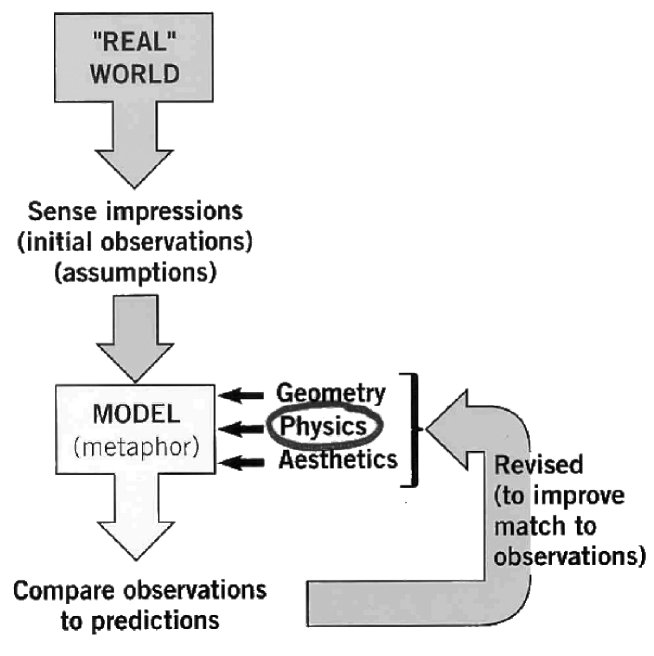
Figure 1: A representation of the logical distinction between reality, observations, and models of reality. Note that the ultimate goal of this process is an improved understanding of the constitutive physics.

1.1 Reality, Models, & Physics

Before I get to that, I would like to step back and take a philosophical look at the general process that we use to learn anything about the objects we study (see Figure 1). Out there somewhere there is a “real world” that we pass through various filters and selection effects to get “observations”. As observers, we try our best to compensate for every effect between the real world and the data point, but it’s important to realize that we use models in this process too.

With the observations in hand, we devise computer models to try to explain them, doing our best to include all of the relevant physical processes that are in principle detectable. Generally these models have a number of tunable parameters, and we do our best to adjust them until the predictions of the model agree as closely as possible with the observations—in our case, generally the pulsation periods of a star. When we have found a model that adequately reproduces the observations, we assume that the values of the parameters tell us something about the properties of the actual star. But we should never forget that what we are actually dealing with are models of reality, and not reality itself. When we derive values of $\log g$ and $T_{\rm eff}$ from spectral lines, for example, we are not measuring the mass and temperature of the star—we are (at best) deriving the optimal match between our models of stellar atmospheres and the extracted spectrum over a finite wavelength interval. We call this approach the “forward method”, and it can only tell us what is best within the context of the models we use. It cannot tell us that we are using the wrong models, unless or until we actually try different models.

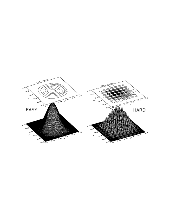
Figure 2: Example model-spaces that would be easy (left) and hard (right) for traditional optimization methods. Note how the likely outcome in the two cases would differ if the search were confined to the region specified by the grey rectangle in the contour plots (Adapted from cha95).

2 Optimization & Objectivity

With this caveat in mind, the process of trying to adjust our model parameters to fit the observations is really just an optimization problem. Mathematicians have devised various methods, each with their strengths and weaknesses, to approach such problems. Imagine that the two axes of the plots shown in Figure 2 represent the two parameters of a model, and that the height of the surface for each combination of parameters is some measure of how well the model matches the observations. If the surface looks like the plot on the left, then just about any optimization method will work. But if the surface looks more like the plot on the right, then most traditional optimization methods will fail miserably, most likely ending up on top of one of the smaller peaks—effectively finding a locally optimal fit, rather than the globally optimal solution. Of course, the trouble is that in general we do not know what the shape of this surface will be for a given model unless we actually evaluate it at each of these points. And that’s exactly what we want to avoid by using an optimization method in the first place: we want the solution as quickly as possible, but we also want it to be the global solution. In section 3.1, I will demonstrate how a genetic algorithm offers a nice tradeoff between these two competing demands.

Before even choosing an optimization method, there is a more fundamental way that we can bias our final result: by defining the range of our search too narrowly. Once again, if the model space is simple, as in the left side of Figure 2, we will probably get a final result at the edge of our search range if we have defined it too narrowly. But if the model space is more complicated, we can find a “global” solution well inside our search range that is not really globally optimal. For this reason, it is important that we define the limits of our search as broadly as possible—constrained only by the physics of the model, and by observations.

For the models of pulsating white dwarfs that I have been using, for example, we adjust five different parameters: the stellar mass, the effective temperature, the mass of the surface helium layer, and two parameters to describe the internal carbon/oxygen profile. Our search range includes masses between 0.45 and 0.95 $M_{\odot}$: white dwarfs with lower masses are expected to have a helium core, and almost all white dwarfs with known masses are below our upper limit Napiwotzki et al. (1999). For now we have been concentrating on the simplest, helium-atmosphere (DB) white dwarfs, so we allow temperatures between 20,000 and 30,000 K, which easily encompasses the spectroscopic temperatures of all known pulsators whether or not trace amounts of hydrogen are included in the atmospheres Beauchamp et al. (1999). We allow the surface helium layer mass to be anywhere from 10${}^{-2}~{}M_{*}$ (a larger mass would theoretically lead to nuclear burning at the base of the layer) down to a few times 10^-8, close to the limit where our models no longer pulsate Bradley & Winget (1994a). We allow the internal composition to range from pure carbon to pure oxygen, and we use the fifth parameter to specify the fractional mass location where the composition begins to change from a uniform C/O mixture in the center, which is what we expect from evolutionary models Salaris et al. (1997). The location of this composition transition is expected to be reasonably close to the half-mass point of the model, but we allow it to be anywhere from 0.1 to 0.85 in fractional mass.

3 Model Fitting

Once we have defined the search range, the only 100% reliable method of finding the globally optimal set of model parameters for a given set of observations is to calculate an entire grid. The main thing to decide at this point is the appropriate resolution of the grid in each parameter. It is common to do this by deciding how long we want to wait for the computer to finish, and which parameters are the most interesting. But even if we had infinite computing power, it makes no sense to calculate a grid so fine that adjacent points give fits that differ by less than the observational noise. A good way to quantify the uncertainties on observed pulsation periods is to identify all of the combination frequencies in the power spectrum, and see how much they differ from what is expected based on the measured parent frequencies.

When we did this for a pulsating DB white dwarf, we found deviations of a few hundredths of a second on pulsation periods that were between 400-800 seconds Metcalfe et al. (2000). This implied that it made sense to calculate about 100 points along each of the five parameters within the ranges specified above. The full grid at this resolution would require 10¹⁰ model evaluations, which would take more than a year to finish even if we had 1000 of today’s fastest processors. If we wanted this kind of resolution for just 1, 2, or possibly 3 of the five model parameters, then maybe a full grid would make sense, especially if we could reuse it for observations of many objects. But certainly for problems with a higher number of free parameters, and to avoid recalculating the grid every few years when the physics gets updated significantly, genetic algorithms can provide almost everything that a grid search can, at a small fraction of the computational cost.

3.1 Genetic Algorithms

The basic idea behind a genetic algorithm is fairly simple: it is just an iterative Monte Carlo method that samples the model space randomly, but keeps a sort of memory of what worked well in the past. It accomplishes this through a computational analogy with the idea of biological evolution through natural selection. The model parameters serve as the genetic building blocks, and the observations provide the selection pressure. It starts just like a simple Monte Carlo, where we generate $N$ random sets of parameters, evaluate the model for each set, and then compare them to the observations. The genetic algorithm treats each set of parameters as an individual in a population, and assigns each a “fitness” based on how well it matches the observations. Next, it selects from this population at random, with the fittest individuals more likely to survive. Here comes the weird part: it encodes the parameters into simple strings of numbers, sort of like chromosomes; it pairs them up and performs operations that are analogous to breeding and mutation, and then decodes the strings back into numerical values for the parameters. Now we have a new population, so we evaluate the model for each case again, and continue the whole process until the population converges to one region of the model space.

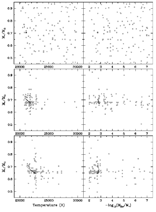
Figure 3: Front and side views of the white dwarf model-space, with snapshots for generation 0 (top), 80 (middle), and 200 (bottom). The best parameter-set in each case is indicated by a black open square, and yields root-mean-square residuals of 4.0, 1.8, and 1.5 seconds in the three panels respectively. The initial convergence is reasonably fast, but the genetic algorithm keeps looking for a better solution, and eventually finds the globally optimal set of model parameters.

This is a bit abstract, so let me illustrate how it works in practice, using a 3-parameter example from the white dwarf problem. The top panel of Figure 3 shows the initial random sample of the model space: each point in the left side of the plot corresponds one-to-one with a point in the right side—this is a front and side view of the model-space. There are 128 points in the sample, and the best one is shown as a black open square. Initially the best root-mean-square (rms) difference between the observed and calculated pulsation periods is 4 seconds, but after 80 iterations (or “generations” of the genetic algorithm) the sample is starting to narrow in on one region of the model-space, and the best solution is substantially better than anything in the original sample. At this point, if we were to compare the observed and calculated periods, we would judge the fit to be pretty good. But as I mentioned at the beginning, in the context of Wampler’s Screwdriver: the genetic algorithm keeps looking. After 200 generations, it has found the globally optimal solution within this modeling framework.

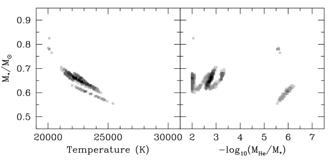
Figure 4: Front and side views of the 3-parameter white dwarf model-space, showing every model evaluated by the genetic algorithm with rms residuals smaller than 3 seconds. The darkness of each point indicates the relative quality of the fit. Note the existence of a second family of solutions with thin helium layer masses.

It is worth noting that along the way to the final solution, the genetic algorithm has evaluated quite a few models, and most of them fall around better-than-average areas of model-space. So, in the end we also get a fairly detailed map giving some sense of the uniqueness of the final solution (see Figure 4). In this case we see that our optimal solution has a relatively thick surface helium layer, but there is also a family of models with thin helium layers that do not match the observations as well, but still match them better than average. This may be telling us something about unmodeled structure in the real star Dehner & Kawaler (1995); Brassard & Fontaine (2002), or possibly about the limitations of the models we are using Montgomery (2002).

3.2 Hare & Hound

One question that I have not answered yet is: how do we decide when to stop the genetic algorithm? The answer is what is usually called a “Hare & Hound” exercise. If you search the Internet for “Hare & Hound”, you will probably find some rather gruesome photographs of a pack of hunting dogs chasing after a little rabbit and collectively ripping it apart when they catch it. I do not like the implication of such an image, but I will use the term anyway. What is usually meant by “Hare & Hound” is a blind test of the analysis method, where you pass simulated data through a process to see how well (and how often) you can recover the input data.

Continuing with our example from the 3-parameter application to white dwarf models, we used the model to calculate the pulsation periods of a theoretical white dwarf with reasonable values for the mass, temperature, and surface helium layer mass. Then we picked out the pulsation periods corresponding roughly to those we had observed in a real white dwarf and used the genetic algorithm to try to find the model parameters that most closely reproduced those periods. Since the genetic algorithm relies on many random processes, it is inevitable that in a finite number of generations it will sometimes fail to find the input model parameters from this test. To quantify the success rate, we repeated this experiment 20 times with different random number sequences Metcalfe et al. (2000). In each case, we saw a rapid improvement after the initial sample, followed by a series of incremental improvements brought about by random processes. Out of the 20 tests, 9 found the exact input parameters within 200 generations, and an additional 4 finished with parameters that were close enough to the input model that a small grid, 11 points on a side, would reveal the exact values. The other 7 runs got stuck in local minima. So, for any given run we have a success probability of the method—genetic algorithm plus small grid—of about 65%. If we only run it once, there is a 35% chance that we will not find the globally optimal solution. But by running it several times, we gradually increase the probability that we will find the globally optimal solution, though we pay for this with more model evaluations. If we do five independent runs, there is a 99.5% chance that we will succeed at least once.

3.3 Problem Scale

The five independent runs, each with 200 generations of 128 trial parameter sets, required that we compute the same number of models as a grid with half the resolution in each dimension. The lesson here is that for small enough problems, the genetic algorithm is not much more efficient than a grid. However, when we scale up to 4 or more parameters, it becomes much more efficient Metcalfe et al. (2001). So our hare and hound test established two things: (1) it told us how many generations we should let the genetic algorithm run, and (2) it implied that there is some minimum problem size that should be attempted with the genetic algorithm—for smaller problems, a model grid might be more efficient.

As an interesting aside, there is also a maximum problem size that should ever be attempted, and this is set by the rate at which computing power increases. There is a well known empirical relation called Moore’s Law, which notes that computing power roughly doubles every 18 months—this has been true since the 1960’s. Because of this trend, if a problem is big enough you can actually get it done faster by waiting for the computing power to increase before you start it. There was a very humorous paper published on astro-ph a couple of years ago on this topic Gottbrath et al. (1999), but the basic conclusions were sound. The authors found that any problem requiring more than 26 months on the fastest computer presently available should not be attempted until the future. As a rule of thumb for the genetic algorithm, a model requiring about 5 minutes to run on today’s fastest available processor will not finish within this 26 month limit on a single machine.

3.4 Parallel Computing

Even if the problem were able to finish in say 24 months, few of us would be willing to wait for two years to get the final answer anyway. Fortunately, we do not have to confine ourselves to one of today’s fastest processors: we can use many of them. This is one of the great things about genetic algorithms—or even model grids for that matter: they are inherently parallelizable. We need to calculate many models, and each of them is independent of the others. So the number of available processors sets the number of models that we can evaluate in parallel. Also, there is very little communication overhead in this process: we send parameter values out to each processor, and we get back either a list of pulsation periods, or just a goodness of fit measure if the periods have already been compared to the observations.

As part of my PhD thesis, I built a 64-processor Linux cluster at the University of Texas Metcalfe & Nather (2000). At the time, dual processor machines were much more expensive than single-processor systems, so it was actually less expensive to have a separate box for each processor. Now, because dual-processor systems are much cheaper, and because computing power has more than quadrupled, we have built a new system that exceeds the speed of the old system in a much smaller space. We can scale this new system up to many more units if we need the computing power—but our problems just don’t demand it yet.

In the future, I would guess that stability and space considerations will be the most important factors for machines like this, and the so-called “bladed Beowulf” concept has already reached the point where it is now possible to put 24 1-GHz processors—none of which require a fan—into a small cabinet the size of a single desktop computer case Feng et al. (2002). The speed of these processors is upgradeable with improved software, written as part of his day job by Linus Torvalds, the creator of the Linux operating system. The big market for these machines, of course, is for massive web servers—but as a nice side-effect they will also provide cheap parallel processing for scientists.

4 Application to White Dwarfs

To give you a sense of the potential of this method, let me summarize what this has done for white dwarf model-fitting. Allowing five adjustable parameters (as outlined in section 2), the genetic algorithm can find the optimal core composition with a precision of a few percent. This is a very significant result in itself, because the core composition can affect the derived ages of white dwarfs by up to 3 Gyr Fontaine et al. (2001), which has implications for using white dwarfs as chronometers to date stellar populations. But the central C/O ratio in a white dwarf formed through single-star evolution can also lead to a measurement of the important ${}^{12}{\rm C}(\alpha,\gamma)^{16}{\rm O}$ nuclear reaction rate.

When a white dwarf is being formed in the core of a red giant star during helium burning, the ${}^{12}{\rm C}(\alpha,\gamma)^{16}{\rm O}$ and 3$\alpha$ reactions compete for the available helium nuclei. As a result, the final central C/O ratio is primarily determined by the relative rates of these two reactions. The 3$\alpha$ rate is relatively well determined, but the ${}^{12}{\rm C}(\alpha,\gamma)^{16}{\rm O}$ reaction is much harder to measure, and so its rate is quite uncertain—leading to a broad range of expected central C/O ratios. By applying the genetic algorithm method, we can now measure the central C/O ratio. By combining this result with evolutionary models that produce internal chemical profiles, we can tune the ${}^{12}{\rm C}(\alpha,\gamma)^{16}{\rm O}$ rate for a model with a given mass until we match the derived central C/O ratio Metcalfe et al. (2002).

We have now applied this method to observations of two pulsating white dwarfs, and in the latest results they both yield a reaction rate consistent with the value derived from laboratory measurements, though they are at best still marginally consistent with each other Metcalfe (2002). We still have more work to do, and crucial tests will come as we apply the method to additional white dwarfs as observations become available. But we have come a long way from the subjective, local model-fitting methods of the past.

5 Conclusions & Discussion

I hope that I have convinced you that genetic algorithms are potentially a very powerful tool for asteroseismology. They can provide objective global optimization for problems with more than a few parameters, and in the process they yield fairly detailed maps of the model-space, which we can use to judge the uniqueness of the final result. To convince yourself that a genetic algorithm is more efficient than a large grid, and to convince others that the final result can be trusted, you should definitely perform a “Hare & Hound” exercise—trying to match your models to the observables from another model, and demonstrating that it can be done. Remember that the speed of your computer effectively determines the size of the problems you can attack. If you want to solve a specific problem, you can and should determine how much computing power you will need to solve it in a reasonable time. Finally, the payoff can be quite high, as it was when we applied this method to our white dwarf models.

I have seen this method begin to transform white dwarf asteroseismology from a field where the theory was being driven by the observations, to one where new observations are being driven by the theory. I hope that it can help launch revolutions in the seismological analysis of other types of stars too.

References

- Beauchamp et al. (1999) Beauchamp, A., et al. 1999, ApJ, 516, 887
- Bradley & Winget (1994a) Bradley, P.A. & Winget, D.E. 1994a, ApJ, 421, 236
- Brassard & Fontaine (2002) Brassard, P. & Fontaine, G. 2002, these proceedings
- Charbonneau (1995) Charbonneau, P. 1995, ApJS, 101, 309
- Dehner & Kawaler (1995) Dehner, B.T. & Kawaler, S.D. 1995, ApJ, 445, L141
- Feng et al. (2002) Feng, W., et al. 2002, LANL Technical Report LA-UR 02-1210
- Fontaine et al. (2001) Fontaine, G., Brassard, P., & Bergeron, P. 2001 PASP, 113, 409
- Gottbrath et al. (1999) Gottbrath, C., et al. 1999, http://arxiv.org/abs/astro-ph/9912202
- Metcalfe (2002) Metcalfe, T.S. 2002, Proc. of the 13th European Workshop on White Dwarfs, ed. R. Silvotti & D. de Martino, in preparation
- Metcalfe & Nather (2000) Metcalfe, T.S., & Nather, R.E. 2000, Baltic Astronomy, 9, 479
- Metcalfe et al. (2000) Metcalfe, T.S., Nather, R.E. & Winget, D.E. 2000, ApJ, 545, 974
- Metcalfe et al. (2001) Metcalfe, T.S., Winget, D.E., & Charbonneau, P. 2001, ApJ, 557, 1021
- Metcalfe et al. (2002) Metcalfe, T.S., Salaris, M., & Winget, D.E. 2002, ApJ, 573, 803
- Montgomery (2002) Montgomery, M.H. 2002, Proc. of the 13th European Workshop on White Dwarfs, ed. R. Silvotti & D. de Martino, in preparation
- Napiwotzki et al. (1999) Napiwotzki, R., et al. 1999, ApJ, 517, 399
- Nather (1995) Nather, R.E. 1995, Baltic Astronomy, 4, 117
- Salaris et al. (1997) Salaris, M., et al. 1997, ApJ, 486, 413
- Wampler et al. (1973) Wampler, E.J., et al. 1973, Nature, 246, 203