Hydrodynamical simulations of the decay of high-speed molecular turbulence. I. Dense molecular regions

Abstract

We present the results from three dimensional hydrodynamical simulations of decaying high-speed turbulence in dense molecular clouds. We compare our results, which include a detailed cooling function, molecular hydrogen chemistry and a limited C and O chemistry, to those previously obtained for decaying isothermal turbulence.

After an initial phase of shock formation, power-law decay regimes are uncovered, as in the isothermal case. We find that the turbulence decays faster than in the isothermal case because the average Mach number remains higher, due to the radiative cooling. The total thermal energy, initially raised by the introduction of turbulence, decays only a little slower than the kinetic energy.

We discover that molecule reformation, as the fast turbulence decays, is several times faster than that predicted for a non-turbulent medium. This is caused by moderate speed shocks which sweep through a large fraction of the volume, compressing the gas and dust. Through reformation, the molecular density and molecular column appear as complex patterns of filaments, clumps and some diffuse structure. In contrast, the molecular fraction has a wider distribution of highly distorted clumps and copious diffuse structure, so that density and molecular density are almost identically distributed during the reformation phase. We conclude that molecules form in swept-up clumps but effectively mix throughout via subsequent expansions and compressions.

1 Introduction

An understanding of turbulence is of fundamental importance to many research areas in astrophysics. In particular, compressible turbulence plays a central role in the process by which stars are formed (reviewed by Vázquez-Semadeni et al. (2000); Padoan et al. (2001)). Stars form out of dense clouds of molecular gas, which have formed out of diffuse clouds of atomic gas. The turbulent energy deduced from observations of the molecular gas is sufficient to delay the gravitational collapse, making molecular turbulence of great interest. The purpose of this study is to provide insight through the first three-dimensional simulations of molecular turbulence.

Isothermal or polytropic equations of state have been the central premise of previous investigations of turbulent models for molecular clouds (e.g. Vázquez-Semadeni et al. (1996); Mac Low et al. (1998); Padoan et al. (1998); Stone et al. (1998)). This simplification has the advantage that parameter space can be explored with numerical simulations, and the influence of magnetic fields and gravity can be determined in some detail (e.g. Balsara et al. (2001); Passot et al. (1995); Klessen (2000); Heitsch et al. (2001) ). The isothermal approximation is indeed valid in many specific models where molecular cooling is efficient and low gas temperatures are maintained. Provided the temperature is low, one can argue that an isothermal equation of state is as good as any other, with little feedback from the the thermal pressure on the dynamics.

However, for cloud formation and evolution molecular chemistry and cooling is critical (Langer et al., 2000; Lim, 2001; Lim et al., 1999). Molecular hydrogen forms most efficiently where the gas is warm but the grains are cool (H₂ forms mainly when atoms combine after colliding and sticking to dust grains). Simple molecules like OH, CO and H₂O form in the gas phase with H₂ as the reactive agent. These molecules are not only important coolants, but associated emission lines provide a means of measuring the cloud properties. Molecules are dissociated as a consequence of fast shocks, UV radiation, X-rays and cosmic rays (Herbst, 2000). We thus need to study molecular turbulence to determine the distribution and abundances of molecular species.

Even in cool optically thin regions, as assumed here, molecular pressures may influence the dynamics. Strong shock waves may be driven from hot atomic regions, formed by shock waves, into the proximity of cold molecular gas. Areas devoid of dust, or in which molecule formation is inefficient (e.g. because atoms will evaporate off warm grains rather than recombine) may attain and maintain pressures as high as turbulent pressures.

The rate of decay of supersonic turbulence is important to the theory of molecular clouds. A possible consequence of the rapid decay of kinetic energy is that the turbulent clouds we observe have short lives. The short lives, however, may not provide sufficient time for relaxation into thermodynamic and chemical equilibrium. Hence, cloud structure and content evolve simultaneously as a cloud evolves dynamically, rather than proceeding through a series of equilibrium states. Therefore, conclusions based on assuming a molecular fraction to be a function of density alone (e.g. Ballesteros-Paredes et al. (1999)) might not always be accurate. We note, however, that the conclusion reached by Ballesteros-Paredes et al. (1999) of rapid cloud formation is supported by this study.

Decaying supersonic turbulence is the subject of this initial study. The work is a direct extension, in terms of code and initial conditions, of isothermal simulations presented by Mac Low et al. (1998). Our goals here are as follows:

• To directly compare the decay of the kinetic energy $E_{kin}$ with those derived in the papers of (Mac Low et al., 1998) and (Smith, Mac Low & Zuev, 2000, 2000).

• To determine the distribution of the molecular column density as opposed to the total column density (Vázquez-Semadeni & García, 2001)

• To study the rate of formation of molecules.

We omit in this study magnetic field, self-gravity and photodissociating radiation. We begin with a fully molecular cube of dense gas and apply an initial turbulent field of velocity perturbations. The turbulence was chosen to be sufficient to dissociate the gas in one case (root mean square (rms) speed of 60 km s^-1) and to leave the gas molecular in another case (rms speed of 15 km s^-1).

2 Methods

2.1 The equations

Numerically we solve the time-dependent flow equations:

$$\frac{\partial\rho}{\partial t}+\nabla\cdot\left(\rho\,\boldsymbol{v}\right) =0,$$ (1)

$$\frac{\partial\left(\rho\,\boldsymbol{v}\right)}{\partial t}+\left(\boldsymbol{v}\cdot\nabla\right)\boldsymbol{v} =-\frac{1}{\rho}\nabla p,$$ (2)

$$\frac{\partial e}{\partial t}+\boldsymbol{v}\cdot\nabla\,e =-p\nabla\cdot\boldsymbol{v}+\Lambda\left(T,n,f\right),$$ (3)

$$\frac{\partial\left(fn\right)}{\partial t}+\nabla\cdot\left(fn\boldsymbol{v}\right) =R\left(T,n,f\right)-D\left(T,n,f\right),$$ (4)

where $n$ is the hydrogen nuclei density, $e$ is the internal energy density and $f$ is the molecular hydrogen abundance (i.e. $n_{\mathrm{H}_{2}}=fn$). We consider the gas as a mixture of atomic and molecular hydrogen with 10% of helium (i.e. $n_{\mathrm{He}}=0.1\,n$). Therefore, the total particle density is $n_{\mathrm{tot}}=(1.1-f)\,n$, mass density is $\rho=1.4nm_{\mathrm{H}}$ and the temperature is $T=p\,/\,(k\,n_{\mathrm{tot}})$. An internal energy loss term has been added to the r.h.s. of the energy flow equation: $\Lambda$ is the loss of energy through radiation and chemistry per unit volume. The function consists of 11 distinct parts, summarised below. $R$ and $D$ are reformation and dissociation rates of molecular hydrogen respectively. A detailed description of the chemistry can be found in Smith & Rosen (2002). Formulae for $\Lambda$, $R$ and $D$ are given in the Appendix A

2.2 The numerical model: ZEUS-3D

As a basis, we employ the ZEUS-3D code (Stone & Norman, 1992a, b). This is a second-order, Eulerian, finite-difference code. We study here compressible hydrodynamics without gravity, self-gravity or thermal conduction. No physical viscosity is modelled, but numerical viscosity remains present, and a von Neumann artificial viscosity determines the dissipation in the shock front.

Further coding for molecular chemistry and molecular and atomic cooling has been added. Our ultimate goal is to develop a reliable code with which we can tackle three dimensional molecular dynamics, later adding self-gravity, magnetic fields, ambipolar diffusion and radiation. We thus restrict the cooling and chemistry lists to just those items essential to the dynamics. We have employed the simultaneous implicit method discussed by Suttner et al. (1997) in which the time step is adjusted so as to limit the change in internal energy in any zone to 30%.

The cooling is appropriate for dense cloud material of any atomic-molecular hydrogen mixture. We include H₂ ro-vibrational and dissociative cooling, CO and H₂O ro-vibrational cooling, gas-grain, thermal bremsstrahlung and a steady-state approximation to atomic cooling (see Smith & Rosen, 2002, Appendix A) and Appendix A of the article.

We take a very basic network of chemical reactions. Time-dependent hydrogen chemistry is included, but C and O chemistry is limited to the reactions with H and H₂ which generate OH, CO and H₂O (see Smith & Rosen, 2002, Appendix B) and Appendix A of the article. Equilibrium abundances are calculated, which are generally accurate within the shocks where molecules are rapidly formed and destroyed. In cold molecular gas, however, the available oxygen will probably remain primarily in the form of water even if it has not been shock-processed. Therefore, the code is constructed to follow the shock-enhanced chemistry and cooling rather than the cold molecular gas. This will generally not be a problem at the high densities where CO cooling and gas-grain heating and cooling determine the properties of the low-temperature gas.

The formula for H₂ formation is critical to the results. Reformation takes place on grain surfaces with the rate taken from (Hollenbach & McKee, 1979):

$$k_{R}=\big{(}3\times 10^{-18}\,[{\rm cm}^{3}{\rm s}^{-1}]\,\big{)}\times\\ \frac{T^{0.5}f_{a}}{1+0.04\,(T+T_{g})^{0.5}+2\times 10^{-3}\,T+8\times 10^{-6}\,T^{2}}$$ (5)

with a factor

$$f_{a}=\big{(}1+10000\exp(-600/T_{g})\big{)}^{-1},$$ (6)

which means, with $T_{g}=20$ K assumed, that $f_{a}$ is quite close to unity in our simulations. Recent experimental results, summarised by Katz et al. (1999), indicate that the H₂ formation rate could be considerably lower. The inherent grain mass and uniform space distribution adopted here also influence the results. This would imply that the absolute reformation times derived here may need revision; we intend to explore a range of possibilities in a following study.

The computations were performed on a Cartesian grid with uniform initial density and periodic boundary conditions in every direction, to simulate a region internal to a molecular cloud. The hydrogen was fixed to be fully molecular at the beginning (fraction: $f=0.5$). Initial stress was introduced by Gaussian perturbations applied to model velocities with a flat spectrum extending over a narrow range of wave numbers given by $3\leq|\boldsymbol{k}|\leq 4$. We have performed runs with root mean square velocities of 15 km s^-1, 30 km s^-1 and 60 km s^-1, and computational domain sizes of 32³, 64³, 128³ and 256³ zones. The number density has been taken to be $n=10^{6}$ cm^-3, physical box size $L=10^{16}$ cm, and the initial temperature has a homogeneous distribution of $T_{i}=100$ K. Abundances for helium, free oxygen and carbon were taken as 0.1, $5\times 10^{-4}$ and $2\times 10^{-4}$.

3 Data analysis

3.1 Decay rates

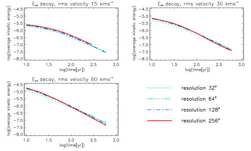
Figure 1: Average kinetic energy as a function of time; log–log plot.

Table 1: Power law indices $\eta$ of kinetic energy decay. The $\eta$ coefficients are derived from linear fitting on the time interval $[90,600]$ years. Average error $\pm 0.006$.

resolution	initial rms velocity for the run
	15 km s-1	30 km s-1	60 km s-1
323	$-1.19$	$-1.33$	$-1.33$
643	$-1.32$	$-1.38$	$-1.36$
1283	$-1.45$	$-1.48$	$-1.52$
2563	$-1.34^{\star}$	$-1.51$	$-1.60$

^⋆ – linear fitting on time interval $[90,300]$ years; the run terminated half way due to numerical difficulties

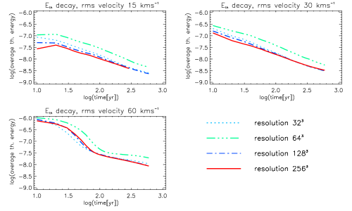
Figure 2: Average thermal energy as a function of time; log–log plot.

Table 2: Power law indices $\mu$ of thermal energy decay. The $\mu$ coefficients are derived from linear fitting performed on the time interval $[90,600]$ years. Average error $\pm 0.008$.

resolution	initial rms velocity for the run
	15 km s-1	30 km s-1	60 km s-1
323	$-0.78$	$-0.82$	$-0.47^{\dagger}$
643	$-0.97$	$-0.99$	$-0.34^{\dagger}$
1283	$-0.82$	$-0.81$	$-0.63^{\dagger}$
2563	$-0.85^{\star}$	$-0.75$	$-0.62^{\dagger}$

^⋆ – linear fitting on time interval $[90,300]$ years; the run terminated half way due to numerical difficulties
^† – linear fitting on the time interval $[140,600]$ years, present final decay behaviour after initial strong cooling regime (see Fig. 2)

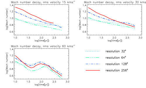
Figure 3: Average Mach number as a function of time; log–log plot.

Table 3: Power law indices $\nu$ of Mach number decay. The $\nu$ coefficients are derived from linear fitting performed on the time interval $[90,600]$ years. Average error $\pm 0.005$.

resolution	initial rms velocity for the run
	15 km s-1	30 km s-1	60 km s-1
323	$-0.08$	$-0.13$	$-0.46^{\dagger}$
643	$-0.16$	$-0.15$	$-0.55^{\dagger}$
1283	$-0.21$	$-0.16$	$-0.49^{\dagger}$
2563	$-0.23^{\star}$	$-0.24$	$-0.54^{\dagger}$

^⋆ – linear fitting on time interval $[90,300]$ years; the run terminated half way due to numerical difficulties
^† – linear fitting on the time interval $[140,600]$ years, present final decay behaviour after initial strong cooling regime (see Fig 3)

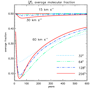
Figure 4: Average molecular fraction as a function of time. There is virtually no dissociation during the run with an initial rms of 15 km s^-1 – all four resolution curves merge in one straight line to the 0.5 level. 30 km s^-1 – intermediate case; 60 km s^-1 – practically all molecules are temporarily destroyed.

The decay in total kinetic energy is displayed in Fig. 1. An initial phase of evolution during which waves steepen and velocity gradients transform into shocks is apparent. The shock formation time is short, with a timescale

$$t_{i}\sim\frac{L}{2\,k_{m}\,v_{rms}}=45.3\times\frac{L}{10^{16}\,{\rm[\mathrm{cm}]}}\frac{10\,[{\rm km\,s}^{-1}]}{v_{rms}}\frac{3.5}{k_{m}}\ [\mathrm{yr}].$$ (7)

where $k_{m}$ is defined as the initial mean wavenumber (Mac Low et al., 1998; Stone et al., 1998; Smith et al., 2000). Hence, shocks develop faster in the 60 km s^-1 turbulent field, as evidenced by the immediate power-law decay.

A rapid power-law decay of kinetic energy with time was uncovered in the isothermal case (Stone et al., 1998; Mac Low et al., 1998; Smith et al., 2000). This actually followed an initial phase of evolution during which velocity gradients increase and shocks appear. The time scale for decay is of the order of a wave crossing time, which implied that turbulent molecular clouds must be short lived if the turbulence is not regenerated.

The first result here is the confirmation that molecular turbulence behaves similar to isothermal turbulence, but with higher rates of decay. The curves of average kinetic energy decay are shown in Fig. 1. Power laws deduced from linear fitting ($\log E_{kin}\propto\eta\log t$) of the curves are shown in Table 1.

We have found that the formula

$$E_{kin}=E_{0}(1+\frac{t}{t_{i}})^{\eta},$$ (8)

fits the data quite well. However, values of $|\eta|$ derived from from fitting the curve (8) are slightly larger due to nonzero values of $t_{i}$. This functional dependence explains why values of the average kinetic energy at the end are compatible, while at the beginning they are different by the factor of 4.

The power-law index $\eta$ increases with $v_{rms}$. This is consistent with the high power-law index found for high Mach number, $M=50$, isothermal turbulence (Smith et al., 2000).

The second result is that the total thermal energy ($E_{th}=nkT(3.3-f)/2$) also decays with time , as opposed to the imposed constant value for the isothermal case. The average thermal energy density behaviour is presented in Fig. 2 and the corresponding decay rates $\mu$: $E_{th}\propto t^{\mu}$ are shown in Table 2. The thermal energy aids our description of the physics. We have found that it also has a power-law decay for the low speed case in which molecules are not destroyed. The thermal energy decays, although not as fast as the kinetic energy. Thus the Mach number remains high relative to the isothermal case, which may well account for the steeper kinetic energy decay rate. Eventually, however, the gas cools down to just below the grain temperature and the turbulent heating input falls off. At this temperature range, however, the numerical code is not accurate enough to resolve the minimum.

The fact that the thermal energy exhibits a dependence on numerical resolution (to a higher degree than kinetic energy does) is due to the importance of cooling layer resolution for the energy balance and smoothening effects on coarser grids. This implies lower values of thermal energy on finer grids, although a smoothening effect for the $64^{3}$ run led to higher (than the $32^{3}$ run) values of the average thermal energy.

With an initial rms speed of 60 km s^-1, the molecules predominantly dissociate within 40 years. Cooling associated with the dissociation and shock heating are competing processes (Fig. 2). After 40 years, there is a steep decay in thermal energy as trace CO and H₂O molecules efficiently cool gas between 100 K and 8000 K. As confirmation, we note that the number of zones within which the temperature is very high ($>10^{3}$ K) falls from a percentage $\approx$ 45% to $\approx$ 1% during the first 150 yr. The gas which had become almost fully atomic (see plots of average molecular fraction in Fig. 4 and histograms on Fig. 5), is again over 60% molecular hydrogen after 300 yr. As the molecules reform, the gas is heated since the molecule energy released on reformation is channelled collisionally into the gas (rather than being radiated) at the high density of these simulations. Therefore, the thermal energy subsequently decays slower than in all other cases, approaching a shallow power-law value. These changes are not directly reflected in the kinetic energy; however, the rapid gas cooling maintains a high Mach number, which leads to the fast decay of kinetic energy.

For reference, the energies are plotted in erg cm^-3, with the initial kinetic energy given by

$$E_{i}=\frac{1}{2}\rho v_{rms}^{2}=1.2\times 10^{-6}\left(\frac{n_{o}}{10^{6}\,[\mathrm{cm}^{-3}]}\right)\times\\ \left(\frac{v_{rms}}{{\rm 10\,[\mathrm{km}\,s}^{-1}]}\right)^{2}[{\rm erg\,cm}^{-3}]$$ (9)

and the final (thermal) energy, after complete molecule reformation ($\gamma=10/7$), is

$$E_{f}=\frac{1}{1-\gamma}n\,k\,T=1.6\times 10^{-9}\frac{n_{o}}{10^{6}\,[\mathrm{cm}^{-3}]}\times\\ \frac{T_{f}}{10\,[\mathrm{K}]}\;[{\rm erg\,cm}^{-3}].$$ (10)

Plots of the average Mach number are shown in Fig. 3, corresponding decay rates, $\nu$: $M\!a\propto t^{\nu}$ are in Table 3. Note that the display is logarithmic, with an average Mach number exceeding 10 maintained for the first 100 yr in the low-speed case. Here we define the average Mach number as

$$M\!a=\sqrt{\frac{\langle\boldsymbol{v}^{2}\rangle}{\langle c_{s}^{2}\rangle}}\,,$$ (11)

where

$$c_{s}^{2}=\frac{(3.5-3f)(2.2-2f)}{(3.3-2f)^{2}}\frac{e}{\rho}$$

is an adiabatic speed of sound, and the bracket notation $\langle\dots\rangle$ means averaging over the domain: $L^{-3}\sum_{i,j,k}$. The Mach number decaying behaviour can be qualitatively explained by noticing that it should be roughly proportional to the fraction $\left(E_{kin}/E_{th}\right)^{1/2}$, although the equality $\nu=(\eta-\mu)/2$ is not generally true.

The increase of the Mach number during the period $\approx[30,120]$ yr in the runs with rms velocity of 60 km s^-1 is due to the strong dissociative cooling at that time, as shown by the thermal energy decay curves, i.e. where $|\mu|>|\eta|$. Note that this case, with the highest initial Mach number, possesses the lowest Mach number once the shocks have formed. This is due to the dissociation, generating a warm atomic gas. The question then is: why do the turbulent motions decay so fast in this case, despite the low Mach number? The suggestion is that the shocks are preferentially running into the denser molecular gas, which can more efficiently dissipate the energy because it is cooler. In isothermal gas, however, this effect would not be apparent.

3.2 Molecular hydrogen evolution

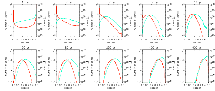
Figure 5: Histograms of the molecular fraction distribution. The black curve corresponds to the left y-axis and represents the volume distribution of molecules: the number of zones with value of molecular fraction within the interval $[f,f+\Delta f]$, $\Delta f=10^{-2}$. The grey curve corresponds to the right y-axis and represents the mass distribution of molecules. The data were taken from the $128^{3}$ run with rms velocity of 60 km s^-1.

Figure 6: Histograms of the average molecular fraction distribution with density at different times. Molecules reform quickly even in regions with low densities. Data from 128³ resolution run with initial rms velocity of 60 km s^-1.

The molecular fraction ‘$f\,$’ is displayed in Fig. 4. The three initial states correspond to three distinct physical regimes. With a rms velocity of 15 km s^-1, very few dissociative shocks develop but some localised dissociation still occurs. With 30 km s^-1, a few per cent of the molecules are dissociated whereas at 60 km s^-1, the gas becomes over 80% atomic.

Note that the minimum value of $f$ is reached after $\sim 4\,t_{i}$. The dynamics alone determines the period of the dissociation phase, which does not overlap with the reformation phase for the chosen parameters.

Reformation of molecular hydrogen is unexpectedly rapid. The expected H₂ reformation time at 20 K and 10⁶ cm^-3 is $t_{R}=(k_{R}\,n_{o})^{-1}$ = 3,200 yr (Eq. 1) a factor of 5 larger than the simulation time. At 100 yr, the temperature is $\sim 80$ K, predicting a reformation time of $t_{R}=(k_{R}\,n_{o})^{-1}$ = 2,000 yr. Yet, reformation is occurring over $\sim 400$ yr. This speed up is caused by the turbulence itself: the molecules preferentially reform in the denser and cooler locations. As weak shocks propagate through the gas, different regions are compressed and expanded. Hence the reformation time is not only controlled by the ‘average’ reformation time, but also by the strength of the turbulence. Given a turbulent dynamical timescale shorter than the average reformation timescale, then we can expect reformation to be accelerated.

We have checked the degree of convergence of both the dissociation and reformation processes. Molecule reformation is a gradual process and is, therefore, accurately represented in the simulations. High resolution is, however, paramount to correctly follow the degree of dissociation. This is critical to the 30 km s^-1 turbulence since there are numerous intermediate speed shocks, partially dissociating the gas. For the low and high speed examples, however, the dissociation is basically zero and complete, respectively. Exhaustive resolution studies of one-dimensional shocks with this code are presented elsewhere (Smith & Rosen, 2002).

The remarkable manner in which the molecular fraction changes is illustrated in Fig. 5 for the high speed case. This figure displays the number of zones $N_{z}(f)$ with a molecular fraction in each interval $[f,\,f\!+\Delta f]$ where $\Delta f$ is taken as 10^-2. After 10 yr, there is an even distribution, suggesting that dissociative shocks have influenced about half the gas. Up to 50 years, the majority of zones have low values of $f$. Thereafter, the reformation has the following properties.

• A single maximum in $N_{z}(f)$ shifts with time to higher values of $f$.

• The maximum remains at $N_{z}\sim 10^{5}$ zones.

• The width of the peak is roughly constant (full width at 80% maximum is 0.16 $\pm$ 0.02)

• The distribution of $f$ by mass displays a single wide peak (grey line in Fig. 5).

• Even in regions with a very low density, reformed molecules are found after 100 yr (Fig. 6).

These vital results imply that $f$ is dominated by a small range in values at any instant, at times after 100 yr. For this reason, three dimensional structure and maps based on column density of either all the gas or just the molecules appear almost identical. In this sense, isothermal simulations can be utilised to determine the structure of molecular clouds or cores but not the underlying fraction of molecules.

3.3 Statistical analysis

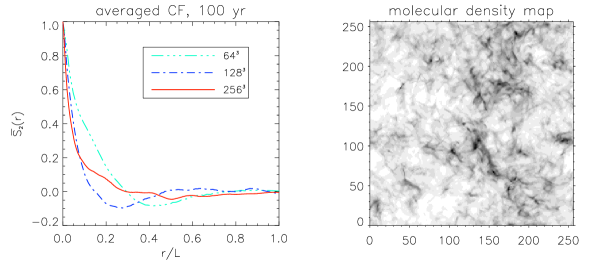
Figure 7: Autocorrelation functions for molecular density and snapshot of molecular density map (from 256³ data) at 100 yr. The molecular density map is the result of the integration of the data cube (fraction $\times$ density) along $z$ axis.

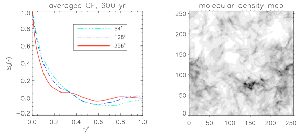
Figure 8: Autocorrelation functions for the molecular density and snapshot of the molecular density map (from 256³ data) at 600 yr. The molecular density map is the result of the integration of the data cube (fraction $\times$ density) along $z$ axis.

Figure 9: The correlation length changes with time in runs with different initial rms velocity. The data taken from the 128³ run. Thick lines represent correlation length, thin line represent inverse average Mach number change.

Figure 10: Probability distribution functions. The left figure presents histograms from the 60 km s^-1 run at 100 yr. The right figure presents histograms from the 30 km s^-1 run at 100 yr. The thicker line corresponds to the averaged PDF from areas with a size of about or less then one correlation length ($\approx 0.23L$), with the associated linear fit coefficient $\kappa_{cr}$. The data are taken from the 256³ run.

In recent years, several studies of probability density functions in numerical simulations have been advanced as a step in their full statistical characterisation (e.g. Vázquez-Semadeni & García (2001); Burkert & Mac Low (2001)). The goal is to quantitatively compare observed maps of the interstellar medium with the predictions of simulations. Here, we present the first analysis of the results for the column density of molecules from turbulent simulations which include the molecular chemistry.

The autocorrelation function is defined as follows:

$$S_{2}(x,y)=\frac{\displaystyle\sum_{i,j}^{L}\big{(}\zeta(i,j)-\langle\zeta\rangle\big{)}\big{(}\zeta(i+x,j+y)-\langle\zeta\rangle\big{)}}{\displaystyle\sum_{i,j}^{L}\big{(}\zeta(i,j)-\langle\zeta\rangle\big{)}^{2}},$$ (12)

where $\zeta(x,y)$ is the quantity (integrated along the LOS):

$$\zeta(x,y)=\frac{1}{L}\sum_{z}^{L}\xi(x,y,z),$$ (13)

where $\xi(x,y,z)$ is the density (or molecular density), and $\langle\zeta\rangle$ is an average:

$$\langle\zeta\rangle=\frac{1}{L^{2}}\sum_{x,y}^{L}\zeta(x,y).$$ (14)

As a qualitative measure, however, it is more convenient to use an averaged correlation function, i.e. polar angle integrated:

$$\bar{S}_{2}(r)=\frac{2}{\pi}\int_{0}^{\pi/2}S_{2}(r\cos{\phi},r\sin{\phi})r\,{\rm d}\phi,\quad r\in[0,L].$$ (15)

Having integrated the correlation function, we have lost all information about anisotropic properties of the molecular density map. However, in our studies we have found that considerable deviations from polar symmetry of a correlation function occur usually only in regions of weak correlation, i.e. separated by a distance which is large in comparison with the correlation length. This suggests that large scale structure which might seem to appear in molecular density maps (e.g. see the map on Fig. 7) is not coherent, and therefore turbulence in the simulations can be considered as isotropic.

We find that the correlation length for the molecular column density grows as the turbulence decays (see Fig. 9 also compare Fig. 7 and Fig. 8) as has been predicted for gas in general by Mac Low (1999) and Mac Low & Ossenkopf (2000). Defining the correlation length as the length over which the average autocorrelation function has decayed by a factor of 10 ($\bar{S}_{2}(\ell_{cr})=0.1$), we find that in the run with resolution of 128³, the correlation length is related to the average sound speed. The growth of $\ell_{cr}$ shows a good correlation with the inverse average Mach number behaviour (see Fig. 9). An explanation for this is easily seen from the following analysis. Defining the crossing time as $t_{cross}=L/\bar{v}$, where $\bar{v}$ is the average speed in the box, we find that the ‘information’ during this time has travelled as much as $\ell_{cr}=\bar{c}_{s}\times t_{cross}$. From this, one immediately obtains the following relation:

$$\frac{\ell_{cr}}{L}=\frac{\bar{c}_{s}}{\bar{v}}\approx M\!a^{-1}.$$ (16)

The autocorrelation functions for density and molecular density maps indeed look very similar, as expected given the above results for the evolution of the molecular fraction within a relatively narrow range of values.

An analysis of the probability density functions (PDF) reveals no particular difference between PDFs for density and molecular density maps and PDFs from different moments of time. Linear fit coefficients $\kappa$ of the histograms of $\zeta$ in log-linear coordinates ($N\propto(\zeta/\zeta_{max})^{\kappa}$) are distributed in a quite wide range: $\kappa\approx[4.0,6.8]$ with a mean value of 5.13 and dispersion $\approx 0.66$ (see Fig. 10).

It has been proposed that observational measurements are often confined to within a correlation length (Burkert & Mac Low (2001)). Linear fit coefficients of the average histograms (mean from a hundred histograms) of regions which have size of about a correlation length, yield a distribution with a smaller dispersion ($\approx 0.22$) and have a mean value of 2.90 (Fig. 10). This is roughly consistent with the observed value for molecular clouds found by Williams et al. (2000); Blitz & Williams (1997). In their studies they have used two-dimensional column density maps of clouds observed in different radial velocity bins for an optically thin molecular species. Each pixel in the data cube (galactic latitude, longitude, radial velocity) has an associated antenna temperature $T_{a}$, proportional to the column density of gas in that pixel. The PDFs was then defined as the total number $N$ of pixels with a certain column density $\zeta/\zeta_{max}$, (where $\zeta_{max}$ is the maximum column density found in the data cube). For molecular clouds in Taurus the following asymptotic value of $\kappa$ is reached: $\kappa=2.7\pm 0.4$. Although our simulations are not directly comparable with the observations of Giant Molecular Clouds, the consistency is quite remarkable.

3.4 Spatial Distribution

In Figs. 11 and 12, we present representations of the three dimensional distributions. These figures demonstrate how the molecular density and total density distributions converge between 50 and 100 yr. Initially, of course, while thermal dissociation is occurring in the shock waves, there is less correlation.

The general structure of the clouds is hard to define. There are some clumps and filament-like structures but little visual evidence for sheets. Some clumps and filaments are surrounded by diffuse envelopes, which are adjacent to other filaments and clumps. Self-gravity or sweeping by large-scale shocks could generate more coherent structures.

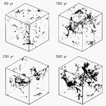
Figure 11: Molecular density distribution snapshots. Data taken from the 128³ resolution run with rms velocity 60 km s^-1. At early stages (when average molecular fraction is low) the distribution of molecular density is different from mass density (see Fig. 12); later, when hydrogen reforms, the distributions look very similar

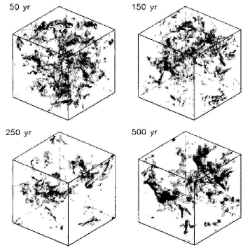
Figure 12: Mass density distribution snapshots. Data taken from 128³ resolution run with rms velocity 60 km s^-1. Compare the distributions with the molecular density distribution on Fig. 11.

4 Conclusions

4.1 Summary

We have presented the properties of a specific model for molecular turbulence. We carried out three dimensional hydrodynamical simulations of decaying supersonic turbulence in molecular gas. We included a detailed cooling function, molecular hydrogen chemistry and equilibrium C and O chemistry. We studied three cases in which the applied velocity field straddles the value for which wholesale dissociation of molecules occurs. The parameters chosen ensure that for the high-speed turbulence, the molecules are initially destroyed in shocks and gradually reform in a distinct phase.

We find the following.

• An extended phase of power-law kinetic energy decay, as in the isothermal case, after an initial phase of slow dissipation and shock formation.

• The thermal energy, initially raised by the introduction of turbulence, decays only a little slower than the kinetic energy.

• The reformation of hydrogen molecules, as the fast turbulence decays, is several times faster than expected from the average density. This is expected in a non-uniform medium, as a consequence of the volume reformation rate being proportional to the density squared.

• The molecules reform into a pattern of filaments and small clumps, enveloped in diffuse structure.

• During reformation, the remaining turbulence redistributes the gas so that the fraction of molecules is distributed relatively evenly. Hence, the density and molecular density are almost identically distributed at any one time after 100 yr.

• The correlation length in our simulations grows with time as has been predicted for a gas in general.

• The probability density functions sampled from regions with size of about one correlation length are consistent with observations.

4.2 Discussion

We mainly wish here to emphasise the insight these simulations provide into how molecular chemistry and supersonic dynamics combine. We have found that isothermal simulations are indeed very useful, not only for the rate of energy decay but also to trace the molecules.

A simple reason for the fast decay is that a sufficient number of strong shocks survive. As shown by Smith et al. (2000), the rate of energy decay in decaying turbulence is dominated by the vast number of weak shocks. These shocks are less efficient at energy dissipation. A second possible reason is that the curved shock structures create small scale vorticity, which leads to enhanced dissipation of kinetic energy. It is not clear, however, why relatively more vorticity should be created when stronger shocks are present. Simulations of isolated curved shocks would help clarify the dissipation paths.

It is plausible that the high Mach number turbulence could create more small-scale structure, leading to a faster decay rates as argued by Mac Low (1999).

The simulations presented here may directly aid our interpretation of fast molecular shocks in dense regions, such as Herbig-Haro objects. For example, supersonic decay would appear to occur in the wake of bow shocks such as in DR 21 (Davis & Smith, 1996). These simulations suggest that the turbulence decays rapidly and bow shock wakes will be bright but short.

The fast reformation of molecules indicates that molecules may form on shorter time scales than previously envisaged. Hence molecular clouds may appear out of atomic clouds several times faster than anticipated in non-turbulent scenarios. Recently, some evidence has been found for rapid cloud formation and dissipation (Ballesteros-Paredes et al., 1999; Hartmann et al., 2001). This implies that much of the interstellar medium may be undergoing both rapid dynamical and chemical changes, driven by sources of supersonic turbulence.

The simulations analysed here provide a basis for much further work. For example, we can now investigate the properties of hydrodynamic clouds in which dust or chemical abundances are non-uniform, clouds in which the turbulence is driven uniformly or non-uniformly, and clouds which are initially atomic.

5 Acknowledgments

The computations reported here were performed using the UK Astrophysical Fluids Facility (UKAFF) and FORGE (Armagh), funded by the PPARC JREI scheme, in collaboration with SGI. M-MML was partially funded by the NASA Astrophysical Theory Program under grant number NAG5-10103 and NFS CAREER grant AST99-85392. AR was funded by the PPARC. Armagh Observatory receives funding from the Northern Ireland Department of Culture, Arts and Leisure. ZEUS-3D was used by courtesy of the Laboratory of Computational Astrophysics at the NCSA.

Appendix A The Chemisitry and The Cooling Function

We consider only a limited network of chemical reactions, which has been tested in one-dimensional simulations (Smith & Rosen, 2002) and which is critical for molecular cloud evolution. These reactions are:

$$\mathrm{H}+\mathrm{H} \longmapsto\mathrm{H}_{2}$$ (17)

$$\mathrm{H}_{2}+\mathrm{H} \longmapsto 3\mathrm{H}$$ (18)

$$\mathrm{H}_{2}+\mathrm{H}_{2} \longmapsto 2\mathrm{H}+\mathrm{H}_{2}$$ (19)

$$\mathrm{O}+\mathrm{H}_{2} \longmapsto\mathrm{OH}+\mathrm{H}$$ (20)

$$\mathrm{OH}+\mathrm{H} \longmapsto\mathrm{O}+\mathrm{H}_{2}$$ (21)

$$\mathrm{OH}+\mathrm{C} \longmapsto\mathrm{CO}+\mathrm{C}$$ (22)

$$\mathrm{CO}+\mathrm{H} \longmapsto\mathrm{OH}+\mathrm{C}$$ (23)

$$\mathrm{OH}+\mathrm{H}_{2} \longmapsto\mathrm{H}_{2}\mathrm{0}+\mathrm{H}$$ (24)

$$\mathrm{H}_{2}\mathrm{O}+\mathrm{H} \longmapsto\mathrm{OH}+\mathrm{H}_{2}$$ (25)

The first three reactions (17, 18, 19) are included in a semi-implicit cooling-chemistry step to calculate the temperature and H₂ fraction. Reaction (17) takes place on grain surfaces with the rate given by equation (5) (see section 2.2).

We fix free oxygen and carbon abundances, $\eta_{0}(\mathrm{O})$ and $\eta_{0}(\mathrm{C})$. We then calculate the equlibrium O, OH, and CO abundances, assuming that the CO reactions are much faster than the H₂O reactions. Then, the remaning free oxygen is distributed into O, OH, and H₂O, according to equlibrium abundances. In this manner we can calculate quite accurately the chemistry within fast shocks without overloading the hydrocode. For further details (see Smith & Rosen, 2002, Appendix B).

The cooling fuction used in the numerical code (see equations 1 – 4 ) is composed of 11 separate parts (one of which heats the gas):

$$\Lambda=\sum_{i=1}^{11}\Lambda_{i}$$ (26)

The components are summarised in Table 4 below.

Table 4: Components of the cooling function

Formulae	Description
$\Lambda_{1}=\lambda_{1}\times n^{2}$, where, on assuming standard dust properties, $$\lambda_{1}=3.8\times 10^{-33.0}T^{0.5}(T-T_{\mathrm{dust}}(1.0-0.8\exp(-75/T))\,\,[\mathrm{erg\,s}^{-1}]$$	gas-grain (dust) cooling (Hollenbach & McKee, 1989). In present calculations we fix $T_{\mathrm{dust}}=20$K.
$\Lambda_{2}=n_{\mathrm{H}_{2}}\left(\frac{L_{v}^{(h)}}{1+L_{v}^{(h)}/L_{v}^{(l)}}+\frac{L_{r}^{(h)}}{1+L_{r}^{(h)}/L_{r}^{(l)}}\right)$, where the vibrational and rotational coefficients at high and low density are: $$L_{v}^{(h)}=1.10\times 10^{-18}\exp(-6744/T)\,\,[\mathrm{erg\,s}^{-1}],$$ $$L_{v}^{(l)}=8.18\times 10^{-13}\exp(6840/T)\left(n_{\mathrm{H}}k_{\mathrm{H}(0,1)}+n_{\mathrm{H}_{2}}k_{\mathrm{H}_{2}(0,1)}\right)\,[\mathrm{erg\,s}^{-1}],$$ the terms $k_{\mathrm{H}(0,1)}$ and $k_{\mathrm{H}_{2}(0,1)}$ are $v:0\rightarrow 1$ collisional excitation rates, $$k_{\mathrm{H}(0,1)}=\begin{cases}1.4\times 10^{-13}\exp(T/125-T^{2}/577^{2}),&\text{if $T<T_{v}$},\\ 1.0\times 10^{-12}T^{0.5}\exp(-1000/T),&\text{if $T>T_{v}$},\end{cases}$$ where $T_{v}$ = 1635 K, $$k_{\mathrm{H}_{2}(0,1)}=1.45\times 10^{-12}T^{0.5}\exp(-28728/(T+1190));$$ $$L_{r}^{(h)}=\begin{cases}\mathrm{dex}\{-19.24+0.474x-1.247x^{2}\},&\text{if $T<T_{r}$ },\\ 3.9\times 10^{-19}\exp(-6118/T),&\text{if $T>T_{r}$ },\end{cases}$$ where $T_{r}$ = 1087 K, and $x=\log(T/10000)$, $$\frac{L_{r}^{(l)}}{Q(n)}=\begin{cases}\mathrm{dex}\{-22.90-0.553-1.148x^{2}\},&\text{if $T<T_{l}$},\\ 1.38\times 10^{-22}\exp(-9243/T),&\text{if $T>T_{l}$},\end{cases}$$ where $T_{l}$ = 4031 K, and $Q(n)=\left(n_{\mathrm{H}_{2}}\right)^{0.77}+1.2\left(n_{\mathrm{H}}\right)^{0.77}$	collisional cooling associated with vibrational and rotational modes of molecular hydrogen. These formulae based on equations 7 – 12 in Lepp & Shull (1983)
$\Lambda_{3}=\left(n_{\mathrm{H}}\right)^{2}\times\lambda_{2}$	collisional cooling of atoms. We have used Table 10 of Sutherland & Dopita (1993) (with $\mathrm{Fe}=-0.5$) for the form of $\lambda_{2}$ and we added an extra thermal bremsstrahlung term equal to $1.42\times 10^{-27}T^{0.5}$ for $T>10^{4}$ K
$\Lambda_{4}=(n_{\mathrm{H}_{2}}+1.39n_{\mathrm{H}})\times n_{\mathrm{H}_{2}\mathrm{O}}\times\lambda_{3}$; $\lambda_{3}=1.32\times 10^{-23}(T/1000)^{\alpha}$ , where $\alpha=1.35-\log(T/1000)$.	cooling through rotational modes of water induced by collisions with both atomic and molecular hydrogen. Given values of $\alpha$ fits the values tabulated by Neufeld & Kaufman (1993)
$\Lambda_{5}=1.03\times 10^{-26}n_{\mathrm{H}_{2}}n_{\mathrm{H}_{2}\mathrm{O}}T\exp(-2325/T)\exp(-47.5/T^{1/3})$	cooling through vibrational modes of water induced by collisions with molecular hydrogen (Hollenbach & McKee, 1989)
$\Lambda_{6}=7.40\times 10^{-27}n_{\mathrm{H}}\lambda_{3}n_{\mathrm{H}_{2}\mathrm{O}}T\exp(-2325/T)\exp(-34.5/T^{1/3})$	cooling through vibrational modes of water induced by collisions with atomic hydrogen (Hollenbach & McKee, 1989)
$\Lambda_{7}=7.18\times 10^{-12}\left((n_{\mathrm{H}_{2}})^{2}k_{D,\mathrm{H}_{2}}+n_{\mathrm{H}}n_{\mathrm{H}_{2}}k_{D,\mathrm{H}}\right),$ where dissociation coefficients are taken to be, $$k_{D,\mathrm{H}}=1.2\times 10^{-9}\exp(-52400/T)\left(0.0933\exp(-17950/T)\right)^{\beta}\,\,[\mathrm{cm}^{3}\,\mathrm{s}^{-1}],$$ $$k_{D,\mathrm{H}_{2}}=1.3\times 10^{-9}\exp(-53300/T)\left(0.0908\exp(-16200/T)\right)^{\beta}\,\,[\mathrm{cm}^{3}\,\mathrm{s}^{-1}],$$ $$\beta=\left[1.0+n\left(2f\left(n_{2}^{-1}-n_{1}^{-1}\right)+n_{1}^{-1}\right)\right]^{-1}$$ critical densities are fit by the following approximation, $n_{1}=\mathrm{dex}\{4.0-0.416x-0.327x^{2}\}\,\,[\mathrm{cm}^{-3}]$ and $n_{2}=\mathrm{dex}\{4.845-1.3x+1.62x^{2}\}\,\,[\mathrm{cm}^{-3}]$.	cooling from the dissociation of molecular hydrogen. Factor $7.18\times 10^{-12}\,[\mathrm{erg}]$ is the 4.18 eV dissociation energy; $n_{1}$ – is the density critical for dissociation by collision of molecular hydrogen with atomic hydrogen, $n_{2}$ – with itself.
$\Lambda_{8}=-\lambda_{7}\xi$, where $\lambda_{7}=k_{R}$ (see Eq. 5) and $\xi=nn_{\mathrm{H}}(1-\beta)7.18\times 10^{-12}$	heating resulting from the reformation of molecular hydrogen. We employ $\beta$ to parametrise the fraction of released energy which is thermalised rather than radiated.
$\Lambda_{9}=n_{\mathrm{CO}}nkT\sigma v_{T}/\left(1+n_{a}/n_{cr}+1.5(n_{a}/n_{cr})^{0.5}\right)$, where the mean speed of the molecules $v_{T}=\sqrt{8kT/(\pi m_{\mathrm{H}_{2}})}$ and $n_{cr}=3.3\times 10^{6}(T/1000)^{0.75}\,[\mathrm{cm}^{-2}]$, $\sigma=3.0\times 10^{-16}(T/1000)^{-0.25}\,[\mathrm{cm}^{-2}]$. Average density, $n_{a}=0.5(n_{\mathrm{H}}+n_{\mathrm{H}_{2}}\sqrt{2})$.	cooling through rotational modes of carbon monoxide induced by collision with both atomic and molecular hydrogen. We based our equations on Eqs. 5.2–5.3 in McKee et al. (1982)
$\Lambda_{10}=1.83\times 10^{-26}n_{\mathrm{H}_{2}}n_{\mathrm{CO}}T\exp(-3080/T)\exp(-68/T^{1/3})$	cooling through vibrational modes of carbon monoxide induced by collisions with molecular hydrogen (see Neufeld & Kaufman, 1993)
$\Lambda_{11}=1.28\times 10^{-24}n_{\mathrm{H}}n_{\mathrm{CO}}T^{0.5}\exp(-3080/T)\exp(-(2000/T)^{3.43})$	cooling through vibrational modes of carbon monoxide induced by collisions with atomic hydrogen

References

- Ballesteros-Paredes et al. (1999) Ballesteros-Paredes J., Hartmann L., Vázquez-Semadeni E., 1999, ApJ, 527, 285
- Balsara et al. (2001) Balsara D. S., Crutcher R. M., Pouquet A., 2001, ApJ, 557, 451
- Blitz & Williams (1997) Blitz L., Williams J. P., 1997, ApJ, 488, L145
- Burkert & Mac Low (2001) Burkert A., Mac Low M.-M., 2001, Column Density Probability Distribution Functions in Turbulent Molecular Clouds: A comparison between Theory and Observations, arXiv:astro-ph/0109447
- Davis & Smith (1996) Davis C. J., Smith M. D., 1996, A&A, 310, 961
- Hartmann et al. (2001) Hartmann L., Ballesteros-Paredes J., Bergin E. A., 2001, ApJ, 562, 852
- Heitsch et al. (2001) Heitsch F., Mac Low M.-M., Klessen R. S., 2001, ApJ, 547, 280
- Herbst (2000) Herbst E., 2000, in Combes F., Pineau des Forêts G., eds, Molecular Hydrogen in Space. The formation of H2 and other simple molecules on interstellar grains.. Cambridge University Press, pp 85–88
- Hollenbach & McKee (1989) Hollenbach D., McKee C. F., 1989, ApJ, 342, 306
- Hollenbach & McKee (1979) Hollenbach D., McKee C. F., 1979, ApJ, 41, 555
- Katz et al. (1999) Katz N., Furman I., Biham O., Pirronello V., Vidali G., 1999, ApJ, 522, 305
- Klessen (2000) Klessen R. S., 2000, ApJ, 535, 869
- Langer et al. (2000) Langer W. D., van Dishoeck E. F., Bergin E. A., Blake G. A., Telens A. G. G. M., Whittet D. C. B., 2000, in Mannings V., Boss A. P., Russel S. S., eds, The University of Arisona Space Science Series, Protostars and Planets IV. The University of Arizona Press, Tuscon
- Lepp & Shull (1983) Lepp S., Shull J. M., 1983, ApJ, 270, 578
- Lim (2001) Lim A. J., 2001, MNRAS, 321, 306
- Lim et al. (1999) Lim A. J., Rawlings J. M. C., Williams D. A., 1999, MNRAS, 308, 1126
- Mac Low (1999) Mac Low M.-M., 1999, ApJ, 524, 169
- Mac Low et al. (1998) Mac Low M.-M., Klessen R. S., Burkert A., Smith M. D., 1998, Phys. Rev. Lett., 80, 2754
- Mac Low & Ossenkopf (2000) Mac Low M.-M., Ossenkopf V., 2000, A&A, 353, 339
- McKee et al. (1982) McKee C., Storey J., Watson D., Green S., 1982, ApJ, 259, 647
- Neufeld & Kaufman (1993) Neufeld D., Kaufman M., 1993, ApJ, 418, 263
- Padoan et al. (1998) Padoan P., Juvela M., Bally J., Nordlund A., 1998, ApJ, 504, 300
- Padoan et al. (2001) Padoan P., Juvela M., Goodman A. A., Nordlund Å., 2001, ApJ, 553, 227
- Passot et al. (1995) Passot T., Vázquez-Semadeni E., Pouquet A., 1995, ApJ, 455, 536
- Smith et al. (2000) Smith M. D., Mac Low M.-M., Heitsch F., 2000, A&A, 362, 333
- Smith et al. (2000) Smith M. D., Mac Low M.-M., Zuev J. M., 2000, A&A, 356, 287
- Smith & Rosen (2002) Smith M. D., Rosen A., 2002, The instability of Fast Shocks in Molecular Clouds, Submitted to MNRAS; http://star.arm.ac.uk/~rar/catinst/
- Stone & Norman (1992a) Stone J. M., Norman M. L., 1992a, ApJS, 80, 753
- Stone & Norman (1992b) Stone J. M., Norman M. L., 1992b, ApJS, 80, 791
- Stone et al. (1998) Stone J. M., Ostriker E. C., Gammie C. F. F., 1998, ApJ, 508, L99
- Sutherland & Dopita (1993) Sutherland R., Dopita M., 1993, ApJS, 88, 253
- Suttner et al. (1997) Suttner G., Smith M. D., Yorke H. W., Zinnecker H., 1997, A&A, 318, 595
- Vázquez-Semadeni & García (2001) Vázquez-Semadeni E., García N., 2001, ApJ, 557, 727
- Vázquez-Semadeni et al. (2000) Vázquez-Semadeni E., Ostriker E. C., Passot T., Stone C. F., 2000, in Mannings V., Boss A. P., Russel S. S., eds, The University of Arisona Space Science Series, Protostars and Planets IV. The University of Arizona Press, Tuscon
- Vázquez-Semadeni et al. (1996) Vázquez-Semadeni E., Passot T., Pouquet A., 1996, ApJ, 473, 881
- Williams et al. (2000) Williams J. P., Blitz L., McKee C. F., 2000, in Mannings V., Boss A. P., Russel S. S., eds, The University of Arisona Space Science Series, Protostars and Planets IV. The University of Arizona Press, Tuscon