Detection of compact objects by means of gravitational lensing in binary systems

We consider the gravitational magnification of light for binary systems containing two compact objects: white dwarfs, a white dwarf and a neutron star or a white dwarf and a black hole. Light curves of the flares of the white dwarf caused by this effect were built in analytical approximations and by means of numerical calculations. We estimate the probability of the detection of these events in our Galaxy for different types of binaries and show that gravitational lensing provides a tool for detecting such systems. We propose to use the facilities of the Sloan Digital Sky Survey (SDSS) to search for these flares. It is possible to detect several dozen compact object pairs in such a programme over 5 years. This programme is apparently the best way to detect stellar mass black holes with open event horizons.

1 Introduction

One of the most important manifestations of gravitational lensing is the visible variability of the astrophysical objects whose emission is affected by the gravitation field of the lens. This effect becomes observable over a reasonable time period, when the velocities of relative motions of the observer, the lens and the source are great enough, i.e. their mutual location changes rapidly. Many cases of this kind of variability have been examined: from light variation of distant quasars to outburst of stars caused by the influence of planets (see, for instance, Zakharov 1997). The brightness variation of the binary system components caused by gravitational lensing was been first considered by Ingel (1972, 1974) and Maeder (1973). They noted that repetition and small characteristic times of the effect make it one of the most accessible to detection and detailed study. It has also been shown (Maeder 1973) that the large amplitudes of brightness variations ($0\aas@@fstack{m}1-0\aas@@fstack{m}5$) can be expected in binary systems consisting of compact objects – white dwarfs, neutron stars, black holes. In fact, only in these cases does the Einstein-Hvol’son radius turn out to be smaller than the lens star radius, and the image of the radiation source is practically not overlapped by it. The latter circumstance makes the gravitational lensing influence in binary systems an effective means for the detection and detailed investigation of compact objects with the aid of photometric methods alone. Their permeability is by $2^{\rm m}-3^{\rm m}$ higher (as compared to spectroscopy), and, therefore, the number of stars amenable to study is an order of magnitude larger. Here the light curve analysis determines all the parameters of the binary system in full analogy to this task for eclipsing binary systems (with allowance made for its singularity) (see, for example, Goncharsky et al. 1985).

A complete set of data for compact object binaries and their statistical analysis gives a possibility to test binary evolution theories and to investigate the last stages of single star evolution as well. We note that only 10 double white dwarfs were detected during the last 10 years (Maxted et al. 2000) and about 40 pairs of a white dwarf and a neutron star – during 25 years (Thorsett & Chakrabarty 1999). We further note that by means of gravitational lensing it is possible to detect compact object binaries at the same rate (see Section 5). Moreover, this may help to discover binaries containing neutron stars with a low magnetic field (not pulsars). Study of these systems in combination with binary star evolution theories gives a possibility to test the detailed cooling models for white dwarfs and neutron stars and the equation of state of the latter (Nelemans et al. 2001; Yakovlev et al. 1999).

Studying compact object pairs is very important to solve a number of astrophysical problems. We present below several such examples.

The ”Standard candle” of modern cosmology, type Ia supernovae, apparently arises from merging of double CO white dwarfs (Webbink 1984; Iben & Tutukov 1984), which have not been detected at this time.

Close double compact objects have to contribute a significant part of the gravitational wave signal at low frequencies. Thus, white dwarf pairs may be a source of the unresolved noise (Evans et al. 1987; Grischuk et al. 2001). Statistical properties of the closest double compact objects in principle determine parameters of the gravitational wave signal.

Binary systems consisting of a white dwarf and a neutron star (a pulsar) are unique laboratories for high-precision tests of general relativity. To date, post-Keplerian general relativistic parameters have been measured in four such pairs (Thorsett & Chakrabarty 1999). This problem may be solved very easily for binaries with gravitational self-lensing since they are observed nearly edge-on.

It seems that the detection of black holes forming pairs with white dwarfs might be an extraordinarily important result of the search for gravitational lensing in compact object binaries. Despite the opinion of most researchers, in a certain sense black holes have not been discovered so far. Only observational data on the behaviour of matter close to the event horizon showing its presence may testify that a black hole is identified (Damour 2000). There is indirect evidence of the presence of black holes in X-ray binaries and galactic cores based on the ”mass-size” relation expected for them (Cherepashchuk 2001). The horizon neighbourhood is seen neither in X-ray binaries nor in the cores of active galaxies because they are screened out by the accreted gas (the accretion rates are very high). This means that only black holes accreting usual interstellar plasma at low rates of $10^{-14}-10^{-15}M_{\odot}$/year can be recognized as objects without a surface and with an event horizon (Shvartsman 1971). The black hole companions of white dwarfs in the binaries detected by means of gravitational lensing could be the best objects for horizon study and tests of general relativity in the strong field limit (Damour 2000). It is very easy to measure the mass and size of such a black hole due to binary edge-on orientation and investigate the radiation of gas near the horizon. This matter is accreted from interstellar medium only because its transfer from the white dwarf is absent.

The gravitational lensing effects in binary systems consisting of compact components were studied previously in several papers (Maeder 1973; Gould 1995; Qin et al. 1997). However, the authors did not go further than estimation of the probability of detecting the effect of orientation of the binary system (often underestimating it by a factor of 2-3), which turned out to be very low. Their general conclusion is that the effect cannot be actually recorded. Nevertheless, the data accumulated by now on the evolution of binary systems and their parameters make it possible to define with higher accuracy the probability of detection of the brightness enhancement in binary systems, to find the expected number of such flares and to propose in the final analysis the strategy for their search based on present-day facilities. Our paper is devoted to performing these tasks.

We examine in Section 2 the distinguishing features of light magnification in the systems consisting of two white dwarfs, a white dwarf and a neutron star, and also a white dwarf and a black hole. In Section 3 we derive probabilities of recording the effect for its different amplitudes in all three cases. In Section 4 the numbers of systems of different types which may be detected by means of gravitational lensing are estimated. In Section 5 we discuss the possibilities of the quest for brightness magnification in such systems with the aid of the telescope and equipment used in the survey SDSS (York et al. 2000).

2 Light curves in gravitational lensing

We will consider three types of binary systems consisting of
a) two white dwarfs with masses of $0.7M_{\odot}$ (sometimes $0.5M_{\odot})$,
b) a white dwarf ($M_{WD}=0.7M_{\odot}$) and a neutron star ($M_{NS}=1.4M_{\odot}$),
c) a white dwarf ($M_{WD}=0.7M_{\odot}$) and a black hole ($M_{BH}=10M_{\odot}$).
It is clear that both components of a pair play the part of a gravitational lens alternately. However, we will mention at once that the source of radiation will always be the white dwarf to which the approximation of a uniformly luminous disk can be applied. The amplitude, the shape and the duration of flares of the lensed object are defined by the relationships between the parameters of the binary system, the major semiaxis $a$, the masses and radii of the components and the orbital plane orientation.

The luminosity magnification of a uniformly radiating disk in gravitational lensing was analysed in detail in the papers by Refsdal (1964), Liebes (1964), Byalko (1969), Ingel (1972, 1974), Maeder (1973) and Agol (2002). On account of the conservation of the surface brightness, the task is reduced in the final analysis to a study of variations of the source image area with allowance made for its occultation by an opaque lens, as the source and lens are moving with respect to the observer (in our case – the orbital motion around the mass centre of the binary system).

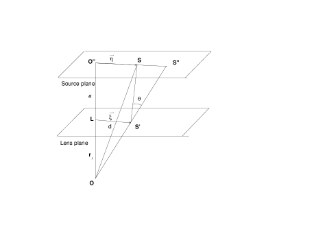
Figure 1: Schematic view of gravitational lensing.

Let $r_{l}$ be the distance from the observer to the gravitational lens, $a$ is the binary system orbit semiaxis (for the sake of simplicity we consider only circular motions), $M_{l}$ is the lens mass, $r_{g}=2GM_{l}/c^{2}$ is its gravitational radius, $R_{l}$ is the lens radius, $R_{s}$ is the source radius, $M_{s}$ is the source mass.

In our case for the light path we can use with high accuracy an approximation of a broken line, the angle between two sections of which is inversely proportional to the impact parameter.

The gravitational lens equation for a point-like source (see, for instance, Zakharov 1997) is

$$\overline{\eta}=\frac{r_{l}+a}{r_{l}}\overline{\xi}-a\overline{\theta}(\overline{\xi}),$$ (1)

where $\overline{\eta}$ and $\overline{\xi}$ are the vectors that characterize the location of the points of intersection of the light ray with the planes of the source and the lens, respectively, $\overline{\theta}(\overline{\xi})$ is the angle of light deflection (see Fig. 1). In our designations $\overline{\theta}(\overline{\xi})=\frac{2r_{g}}{\xi}\cdot\frac{\overline{\xi}}{\xi}$. The main parameter of the task is the Einstein-Hvol’son radius $r_{e}=\sqrt{2r_{g}\frac{ar_{l}}{r_{l}+a}}$, the radius of the ring - the image of the point source, lying on the ”observer – lens” axis in the lens plane. In our case $r_{l}\gg a$ and

$$r_{e}=\sqrt{2r_{g}a}$$ (2)

or, in solar units,

$$r_{e}=3\cdot 10^{-3}M^{1/2}a^{1/2}.$$

Equation (1) has two solutions and hence the source images are two points in the lens plane with coordinates:

$$\xi_{1,2}=\frac{d}{2}\left(1\pm\sqrt{1+\frac{4r_{e}^{2}}{d^{2}}}\right),$$ (3)

where $d=|\overline{\eta}|$ is the ”lens–source” vector projection onto the lens plane, i.e. displacement of the source off the ”observer–lens” axis.

For the magnification coefficient $K$, i.e. the ratio of the sum of brightness of the two images to the point-like source brightness, we have (Zakharov 1997)

$$K=\left|\frac{\xi d\xi}{\eta d\eta}\right|_{1}+\left|\frac{\xi d\xi}{\eta d\eta}\right|_{2}=\frac{1}{2}\left(\sqrt{1+\frac{4r_{\rm e}^{2}}{d^{2}}}+\frac{1}{\sqrt{1+\frac{4r_{e}^{2}}{d^{2}}}}\right).$$ (4)

To evaluate the possibility of using particular approximations, it is necessary to estimate the values of the task parameters. As has already been mentioned, we consider only the white dwarf as a source of radiation. The role of the lens is played by a white dwarf (WD), a neutron star (NS) or a black hole (BH). At typical velocities of the orbital motion, 100–300 km/s, the accretion luminosity of the BH is $10^{3}-10^{5}$ as low as the thermal luminosity of the WD (Ipser & Price 1982). Assuming $M_{WD}=0.7M_{\odot},M_{NS}=1.4M_{\odot},M_{BH}=10M_{\odot},R_{NS}=15,R_{BH}=r_{g}=2GM_{BH}/c^{2}$, we have estimated the rest of the parameters of binary systems, which are presented in Table 1 in solar units.

Table 1: Einstein radii for different binary systems

Pair	$M_{l}$	$R_{l}$	$r_{e}$		$R_{s}$
	$(M_{\odot})$	$(R_{\odot})$	($R_{\odot}$)		$(R_{\odot})$
			$a=10$	$a=100$
WD+WD	0.7	$10^{-2}$	$1.0\cdot 10^{-2}$	$3\cdot 10^{-2}$	$10^{-2}$
WD+NS	1.4	$2\cdot 10^{-5}$	$1.1\cdot 10^{-2}$	$3.5\cdot 10^{-2}$	$10^{-2}$
WD+BH	10	$4\cdot 10^{-5}$	$3\cdot 10^{-2}$	$9.5\cdot 10^{-2}$	$10^{-2}$

For the WD radius we used the relationship (Nauenberg 1972):

$$R=0.01125R_{\odot}\left(\left(\frac{M}{1.454M_{\odot}}\right)^{-\frac{2}{3}}-\left(\frac{M}{1.454M_{\odot}}\right)^{\frac{2}{3}}\right)^{\frac{1}{2}}.$$ (5)

One can see that in a system of two WDs, the Einstein radius, the sizes of the lens and the source are close. This implies that when considering the light magnification one has to take into account the source extension and occultation of its image by the companion – the lens, at least, at $a<100R_{\odot}$, which, as we will see, is our primary interest. In binary systems, containing a NS and a BH, eclipsing is absent; the source, however, can be regarded as a point one only at $a>(10-20)R_{\odot}$, and one can apply expression (4) to derive the brightness increase.

It should be noted that when the binary system is viewed edge-on, at the moment of conjunction, a configuration in which the observer, the lens and the source are on one line $(d=0)$ is realized. It was shown (Liebes 1964) that in this case $K=\sqrt{1+\frac{4r_{e}^{2}}{R_{s}^{2}}}$, as a result of averaging of expression (4) over the surface of the uniformly radiating disk. At $d\neq 0$ the task gets essentially more complicated and has no analytical solution. The accurate relationships for the brightness magnification by a point lens, where elliptical Legendre integrals of the first and second kinds are used, were derived by Refsdal (1964), Liebes (1964), Byalko (1969), Ingel (1972, 1974) and Maeder (1973). There is, however, one more case in which a simple expression for $K$ exists – the contact between the disk edge and the lens centre:

$$\begin{array}[]{ll}K&=\frac{2}{\pi}\left[1+4(\frac{r_{e}}{R_{s}})^{2}\right]\arcsin\left[1+4(\frac{r_{e}}{R_{s}})^{2}\right]^{-\frac{1}{2}}\\ &\\ &\approx\frac{2}{\pi}\sqrt{1+4\beta^{2}}\,,\end{array}$$ (6)

where $\beta=\frac{r_{e}}{R_{s}}$.

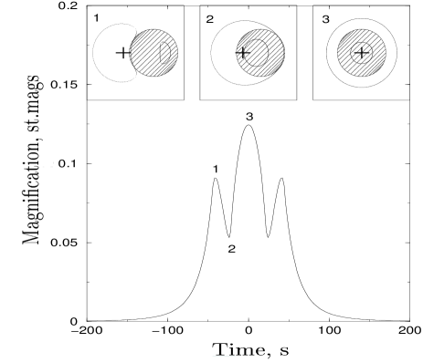
Figure 2: Magnification curve for the pair of white dwarfs. The crosshatched circle is the gravitational lensing component.

The light curve of the component-source is the result of variation of magnification with time variations of $d$ during the system rotation period. In the approximation of a point source, according to (4)

$$K(t)=\frac{1}{2}\left[\sqrt{1+\frac{4r_{e}^{2}}{d(t)^{2}}}+\frac{1}{\sqrt{1+\frac{4r_{e}^{2}}{d(t)^{2}}}}\right].$$ (7)

Near the conjunction $d^{2}(t)=d_{0}^{2}+(vt)^{2}$, where $d_{0}=a\sin i$ is the minimum value of $d$, which depends on the orbit inclination $i$, $v$ is the ralative velocity of the system components. At the moment $t=0$, the brightness variation reaches a maximum and

$$\begin{array}[]{ll}K_{m}&=K(0)=\frac{1}{2}\left[\sqrt{1+\frac{4r_{e}^{2}}{d_{0}^{2}}}+\frac{1}{\sqrt{1+\frac{4r_{e}^{2}}{d_{0}^{2}}}}\right]\\ &\\ &=\frac{1}{2}\left[\sqrt{1+4\beta_{0}^{2}}+\frac{1}{\sqrt{1+4\beta_{0}^{2}}}\right],\end{array}$$ (8)

here $\beta_{0}=\frac{r_{e}}{d_{0}}$.

It is customary to characterize the duration of the flare (brightness increase) (see Zakharov & Sazhin 1998) by the time $\tau$ that is taken by the moving source projection onto the lens plane to cross the Eintstein ring. It can be easily found from the relation $d^{2}(\frac{\tau}{2})=d_{0}^{2}+(\frac{v\tau}{2})^{2}=r_{e}^{2}$, that:

$$\tau=\frac{2r_{e}}{v}\sqrt{1-\frac{1}{\beta_{0}^{2}}}.$$ (9)

In a point approximation $K(\frac{\tau}{2})=\frac{1}{2}[\sqrt{5}+\frac{1}{\sqrt{5}}]\doteq 1.34$, and $\tau$ defines the flare duration at a level $\Delta m_{0}=0\aas@@fstack{m}32$ of the source light at a quiescent phase.

Note that the brightness magnification of one of the components by a factor of $K$ corresponds to magnification of the system brightness (which is the subject of detection in observations) $K_{0}$ times, and

$$K=K_{0}+\frac{L_{l}}{L_{s}}(K_{0}-1),$$ (10)

where $\frac{L_{l}}{L_{s}}$ is the lens–source brightness ratio. For a system containing two equal white dwarfs $\frac{L_{l}}{L_{s}}=1$, $K_{0}=\frac{1}{2}(K+1)$, and $\Delta m_{0}=0\aas@@fstack{m}17$ with respect to the total system brightness off the flare. It is self-evident that if the part of the lens is played by a neutron star or a black hole, the $K$ is practically equal to $K_{0}$.

Present-day telescopes detect rather small light variations during short exposures (see Section 5). We are guided by these possibilities when determining the minimum amplitude of detectable flares. Say, if the amplitude of a flare $\Delta m_{0}=0\aas@@fstack{m}2$ ($K=1.2$), then the trajectory of the source projection onto the lens plane does not cross the Eintstein ring at all, and such a flare is excluded from the analysis. Therefore, it is necessary to introduce $\tau_{0.1}$ at which $K=1.1$. Using (4) we derive

$$(\frac{r_{e}}{d})^{2}=\beta^{2}=\frac{K^{2}-1+K\sqrt{K^{2}-1}}{2},$$ (11)

hence at $K=1.1,\beta_{0.1}=0.60$, $d_{0.1}=1.67r_{e}$. Thus

$$\tau_{0.1}=1.67\frac{2r_{e}}{v}\sqrt{1-\frac{1}{(1.67\beta_{0})^{2}}}.$$ (12)

In the general case, when deriving the light curves, equation (1) was solved for each point of the source profile, its image was constructed in the lens plane, and its area was found numerically. Since in gravitational lensing, the surface brightness remains constant, the light curve is determined as variation of the ratio of the image areas and the source itself, depending on the position of the binary system components with respect to the observer, which varies during the period of rotation. The contribution to the system radiation of the lens–white dwarf and occultation by it of a part of the source image was taken into account. Fig. 2 shows the brightness variations of the binary system consisting of two white dwarfs with a mass of $0.7M_{\odot}$, $a=14.2R_{\odot}$ and the orbit inclination $i=0$ (i.e. $d_{0}=0$). The similarity of the sizes of the source, the lens and the Einstein ring results in formation of a rather complex light curve. Similar events were analysed by Marsh (2001) and Agol (2002).

Comparison of the light curves in Fig. 3, plotted from the use of the results of direct calculations and with the use of point approximation (7), shows that they are virtually coincident for $a>30R_{\odot}$. In this case the light curves can be constructed by means of a point approximation. The exception is the region near the maximum at $\frac{d(t)}{r_{e}}<0.25$.

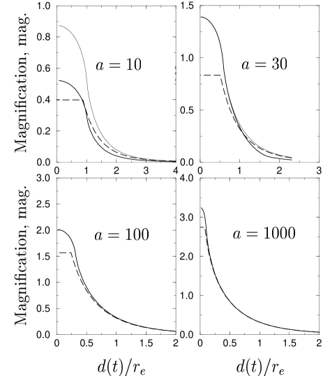
Figure 3: Magnification curves of the pair of white dwarfs for different semiaxes $a$. Dashed lines represent the analytical approximation (7). Solid lines for numerical calculation; fine ones for transparent lens, thick ones for opaque lens.

Consider the effect of gravitational lensing in a binary system comprising two equal white dwarfs with $M_{WD}=0.5M_{\odot}$ and $a=100R_{\odot}$. According to Kepler’s third law (in solar units):

$$T=2.79a^{3/2}(M_{l}+M_{s})^{-\frac{1}{2}}\;{\rm hours},$$ (13)

its period $T=82.4$ days. Flares which amplitude depends on $i$ will be observed twice during this time. For $d_{0}\approx ai>R_{s}$, point approximation (8) can be employed to estimate the amplitude. Consequently, at $i>\frac{R_{s}}{a}=\frac{10^{-2}}{10^{2}}=10^{-4}$, it follows from (2) and (8)

$$K_{m}=\frac{1}{2}\left[\sqrt{1+\frac{4}{i^{2}}\cdot\frac{2r_{g}}{a}}+\frac{1}{\sqrt{1+\frac{4}{i^{2}}\frac{2r_{g}}{a}}}\right]\leq 2.27.$$

Thus the amplitude of these flares $K_{0}=\frac{1}{2}(K_{m}+1)\leq 1.64$ or $\Delta m_{0}\leq 0.54$.

From (2) and (9), considering that $v=\sqrt{\frac{G(M_{l}+M_{s})}{a}}$, obtain under the same condition (point approximation):

$$\tau=\frac{4a}{c}\sqrt{\frac{M_{l}}{M_{l}+M_{s}}}\cdot\sqrt{1-\frac{i^{2}a}{9\cdot 10^{-6}M_{l}}}.$$ (14)

And for the given system $\tau=\frac{4a}{c\sqrt{2}}\sqrt{1-\frac{i^{2}a}{4.5\cdot 10^{-6}}}=662\sqrt{1-2.2\cdot 10^{7}\cdot i^{2}}$ sec.

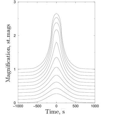
Figure 4: Simulated light curves of the pair of white dwarfs.

In Fig. 4 the light curves of this system for different $i$, plotted from the data of numerical computations, are displayed. The light variations are expressed in stellar magnitudes. The orbit inclination $i$ varies from zero to $2.5\cdot 10^{-4}$ with a step of $2.5\cdot 10^{-5}$ from the upper to the lower curve, which is displaced for convenience. The flare shape variations are due to these changes.

Table 2: Parameters of the closest pairs able to give rise to a flare of amplitude $\Delta m$

$\Delta m$	WD+WD			WD+NS			WD+BH
	$a_{min}$	$a_{c}$	$\tau_{0.1}$	$a_{min}$	$a_{c}$	$\tau_{0.1}$	$a_{min}$
	($R_{\odot}$)	($R_{\odot}$)	(s)	($R_{\odot}$)	($R_{\odot}$)	(s)	($R_{\odot}$)
$0\aas@@fstack{m}2$	4	14	44	0.92	2.5	12	0.13
$0\aas@@fstack{m}5$	15.4	23	170	3.15	3.2	41	0.44
$1\aas@@fstack{m}0$	62.4	49	690	11	10	141	1.52

One more step brings us closer to the real condition of searching for flares. Having fixed three levels of brightness increase, $0\aas@@fstack{m}2$, $0\aas@@fstack{m}5$ and $1\aas@@fstack{m}0$, we determined by two methods the minimum sizes of the systems consisting of two white dwarfs and also a white dwarf and a neutron star whose light rises to these levels (Table 2). From the relation $K=\sqrt{1+\frac{4r_{e}^{2}}{R_{s}^{2}}}$, $a_{min}$ has been found analytically, while $a_{c}$ has been derived by direct calculations. The light curves of flares in these edge-on-viewed pairs, which were constructed based on numerical computations, are presented in Fig. 5a, b. It can be seen from Table 2 and this figure that the analytical estimates of the characteristic durations of flares $\tau_{0.1}$ are close to the results of direct calculations. The flares of a white dwarf coupled with a black hole constructed in a similar manner are exhibited in Fig. 5c (Table 2 contains only $a_{min}$ for this binary system), here the separation of the components $a=3R_{\odot}$, while the amplitudes $0\aas@@fstack{m}2,0\aas@@fstack{m}5,1\aas@@fstack{m}0$ correspond to the orbital plane inclinations 0.023, 0.015 and 0.01. It is precisely this value of $a$ that was used in the computation since it is close to the minimum size of the pair WD–BH, which ”survived” in the process of emission of gravitation waves during the lifetime of the Galaxy. The number of closer pairs drops sharply and the probability of their detection is very low (see Section 3).

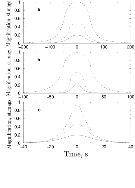
Figure 5: Simulated light curves of the flares as a result of gravitational lensing in different pairs: a)  WD–WD, b)  WD–NS, c)  WD–BH. Dashed lines show flares with amplitude $1\aas@@fstack{m}0$, dotted lines are used for flares with amplitude $0\aas@@fstack{m}5$ and solid lines for flares with amplitude $0\aas@@fstack{m}2$.

Fig. 5a, b, c shows that the characteristic durations of flares for pairs of white dwarfs are 50–200 s; for binaries containing NS and BH, the light variations are shorter, 30–130 s and 20–40 s, respectively. Singnificant variations of the flare shape are noticeable in all the cases.

Without dwelling on details, note that the set of parameters of these binary systems obtained in observations – light curves, periods, amplitudes, duration and shape of flares, can make it possible to determine physical characteristics of the components – their masses, sizes, temperatures (e.g. Cherepashchuk & Bogdanov 1995a, b). This problem can be resolved completely for two white dwarfs. At the same time, the determination of, at least, the mass of the lens component and, therefore, its identification as a NS or a BH seems to be self-important for the study of properties of relativistic objects and their extreme gravitation fields.

3 Probability of detection of flares and their average characteristics

The number of systems that can be found as a result of brightness increases in gravitation lensing is determined, first of all, by the probability $F(K_{0},t)$ of recording a flare with an amplitude larger than the level $K_{0}$, during the observing time $t$ of a sample of systems distributed in some manner over parameters (orbital separation, masses and component brightness). This means that $F(K_{0},t)$ is the probability of a flare detection from a certain system averaged over such a distribution

$$F(K_{0},t)=\int\limits_{\Omega}P(K_{0},t,\omega)f(\omega)d\omega,$$ (15)

where $\omega$ is the set of parameters, $f(\omega)$ is the function of their distribution, $\Omega$ is the region in which they are specified, $P(K_{0},t,\omega)$ is the probability of recording of the flare in a system with the parameters $\omega$. For the sake of simplicity, with allowance made for the low accuracy of any estimates associated with statistical characteristics of binary systems with compact companions (Masevich & Tutukov 1988; Lipunov et al. 1996; Nelemans et al. 2001; Fryer et al. 1999, where the errors of different models are defined), we restrict ourselves to an analysis of the distribution of the systems only in $a$. Then $P(K_{0},t,a)$ is the probability of a joint onset of two events, favourable orientation of the orbital plane with the semiaxis $a$, when the level $K_{0}$ in the flare is exceeded, and the recording of a result if only one such a flare occurs during the time $t$, $f(\omega)d\omega=f(a)da$.

The first event is consistent with the geometric probability $p_{g}$ which can be easily found. It follows from (4), (7), (8) and (11) that the values $d_{0}^{\prime}<d_{0}=\frac{r_{e}}{\beta(K)}$, where $K=K_{0}+\frac{L_{l}}{L_{s}}(K_{0}-1)$, correspond to the flares of the source with amplitudes exceeding $K$. The locus of the ends of the normals of the orbital planes satisfying this condition is a globe belt of width $d_{0}$ and radius $a/2$, its area is $S_{d}=\pi ad_{0}$. The locus of the ends of the normals of any orbit is the surface of a sphere of radius $\frac{a}{2}$, its area is $S_{a}=\pi a^{2}$. Hence $p_{g}=\frac{S_{d}}{S_{a}}=\frac{d_{0}}{a}=\frac{r_{e}}{a\beta(K)}$. Finally, from (2) $p_{g}=3\cdot 10^{-3}a^{-\frac{1}{2}}M_{l}^{\frac{1}{2}}[\beta(K)]^{-1}$.

Note that in determining $\beta(K)$, both analytical expression (11) and the numerical relationship can be applied. Fig. 6 shows the relationships between geometric probabilities and the size of a system consisting of two white dwarfs which have been derived by these two methods (analytically in a point approximation – the dashed line, and numerically – the solid one). The contribution of the dwarf lens is taken into account here. Minimum sizes of systems capable of giving rise to a flare of amplitude $K$ correspond to the values $a_{c}$ in Table 2. The numerical calculations in systems WD–NS and WD–BH are virtually the same as the analytical estimates, but $p_{g}$ for WD-NS reduces to zero at $a=a_{c}$.

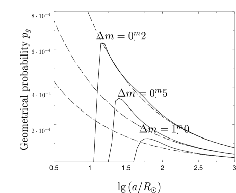
Figure 6: Geometrical probability versus semiaxis size for the pair of white dwarfs. Dashed lines for analytical approximation, solid lines for numerical calculation.

The probability $p_{t}$ of recording a flare during the time $t$ is essentially dependent on the relationship of the period of recurrence of flares $T$ (given by (13)), the duration of the flare $\tau$ and the net continuous time of observing $t$. Let us lay down certain conditions which must be satisfied to make the search for flares efficient enough. First of all, it is evident that the duration of an elementary continuous exposure $t_{e}$ must be close to that of flare $\tau$. On the other hand, the interval between the exposures must be considerably shorter than $\tau$. Implying by $t=\sum\limits_{e}t_{e}$ the duration of the total exposure when observing a specified sky region, we obtain for the probability $p_{t}$:

$$p_{t}=\left\{\begin{array}[]{ccc}\frac{t}{T}&{\rm at}&t<T\\ 1&{\rm at}&t>T,\\ \end{array}\right.$$ (16)

which corresponds to

$$p_{t}=\left\{\begin{array}[]{ccl}0.36\frac{t(M_{l}+M_{s})^{1/2}}{a^{3/2}}&{\rm at}&a>a_{t}\\ 1&{\rm at}&a<a_{t},\hskip 76.82234pt(16^{\prime})\\ \end{array}\right.$$

where $a_{t}=[0.36t(M_{l}+M_{s})^{1/2}]^{2/3}$ is the semiaxis of binary with period $T=t$ and we consider $a_{t}\geq a_{c}$ only since $p_{g}=0$ as $a<a_{c}$.

Hence

$$\begin{array}[]{l}P(K_{0},t,a)=p_{g}p_{t}\\ \;=\left\{\begin{array}[]{lll}0,&{\rm at}&a<a_{c},\\ 3\cdot 10^{-3}a^{-\frac{1}{2}}M_{l}^{1/2}[\beta(K)]^{-1}&{\rm at}&a_{c}<a<a_{t},\\ &&\\ 1.08\cdot 10^{-3}ta^{-2}\frac{[M_{l}(M_{l}+M_{s})]^{1/2}}{\beta(K)}&{\rm at}&a_{c}<a;\\ &&a_{t}<a.\\ \end{array}\right.\end{array}$$ (17)

Due to the serious anisotropy of pair distributions on the sky, the optimum time of observation of a specified sky field will be shown to be greater than one night length (at least for WD-WD systems). In this case a simple expression (16) for $p_{t}$ no longer holds since observations on individual nights become statisticaly independent. The probability of detecting at least one flare in $n$ nights is given by the Bernoulli distribution:

$$p_{n}=1-(1-p_{1})^{n}=\sum\limits_{1}^{n}(-1)^{i+1}C_{n}^{i}p_{1}^{i}.$$

where $p_{1}=p_{t}|_{t=9^{h}}=3.24(M_{l}+M_{s})^{1/2}a^{-3/2}$ is the detection probability in $9^{h}$ (the observational night average length).

Thus, expression for $P(K_{0},n,a)$ takes the following form

$$\begin{array}[]{l}P(K_{0},n,a)=p_{g}p_{n}\\ \;=\left\{\begin{array}[]{lll}0,&{\rm at}&a<a_{c}\\ 3\cdot 10^{-3}a^{-\frac{1}{2}}M_{l}^{1/2}[\beta(K)]^{-1},&{\rm at}&a_{c}<a<a_{1}\\ 3\cdot 10^{-3}M_{l}^{1/2}[\beta(K)]^{-1}&&\\ \times\sum\limits_{1}^{n}(-1)^{i+1}(3.24)^{i}C_{n}^{i}&&\\ \times(M_{l}+M_{s})^{i/2}a^{-\frac{1}{2}(3i+1)}&{\rm at}&a_{1}<a,\hskip 36.98866pt(17^{\prime})\end{array}\right.\end{array}$$

where $a_{1}=a_{t}|_{t=9^{h}}=2.2(M_{l}+M_{s})^{1/3}$.

For randomization corresponding to (15) we must convolve $P(K_{0},t,a)$ or $P(K_{0},n,a)$ with the pair distribution function in $a$.

Now we turn to the analysis of this distribution. We must clearly see the difference in distribution for binary systems, progenitors of pairs of compact objects, and the finite distribution of these pairs themselves. In the first case the results of observations yield a distribution uniform in logarithm of semiaxis (Abt 1983): $f(a)\propto a^{-1}(1\leq\log(a/R_{\odot})\leq 6)$. In the second case the situation is not so clear because of the uncertainty in quantitative characteristics determined in the course of different versions of population synthesis and because of the qualitative distinctions of these versions (Yungelson et al. 1994; Lipunov et al. 1996; Saffer et al. 1998; Portegies Zwart & Yungelson 1998; Fryer et al. 1999; Nelemans et al. 2001). For instance, in different papers the initial mass functions with different indices are used; due to the great uncertainty in the loss of matter, the supposed masses of BH progenitors vary from $25M_{\odot}$ to $80M_{\odot}$. The finite numbers of, say, couples WD–BH contain an uncertainty of 5 orders of magnitude (see Fryer et al. 1999)! Nevertheless, since our analysis is qualitative, one can be content with the main characteristics of samples of objects and rough estimates.

First of all, it will be noted that couples lose energy and angular momentum radiating gravitation waves (Landau & Livshits 1983; Grishchuk et al. 2001). Since the rate of these losses depends dramatically on $a\;(\propto a^{-5})$, the stars in close pairs stick together and leave the sample. Using the expression for gravitational luminosity of a binary system in a circular orbit $\frac{dE}{dt}=-\frac{32}{5}\frac{G^{4}}{c^{5}}\cdot\frac{M_{l}^{2}M_{s}^{2}(M_{l}+M_{s})}{a^{5}}$ (Landau & Livshits 1983) and taking into account that the total energy of the system $E=-\frac{GM_{l}M_{s}}{2a}$, one can readily derive the value of $a_{r}$ of the initial semiaxis of a system that will merge during $10^{10}$ years, which is the life-time of the Galaxy:

$$a_{r}=2R_{\odot}[M_{l}M_{s}(M_{l}+M_{s})]^{1/4}.$$

We tabulate in Table 3 the values of $a_{r}$ and corresponding $T_{r}$ for the systems under study.

Table 3: The closest pairs that survived during the life-time of the Galaxy

Pair	$M_{l}+M_{s}$	$a_{r}$	$T_{r}$
	($M_{\odot}$)	($R_{\odot}$)	(hours)
WD+WD	0.7+0.7	1.82	5.77
WD+NS	0.7+1.4	2.40	7.11
WD+BH	0.7+10	5.88	12.13

The results of population synthesis, which are partially confirmed by observations, suggest that the density destribution of pairs of compact objects rises with decreasing $a$ approximately as $\frac{1}{a}$, reaches a maximum at $a=a_{0}\sim a_{r}$, after which it decreases rapidly to $a\sim 1R_{\odot}$ (Lipunov et al. 1996; Hernanz et al. 1997; Saffer et al. 1998; Portegies Zwart & Yungelson 1998; Wellstein & Langer 1999).

It follows from the same papers that another important parameter, the maximum size of a binary system $a_{max}$, is known to be less than $50R_{\odot}$ at small eccentricities.

With allowance made for the said above, we have used the function of distribution in $a$ in a simple form:

$$\begin{array}[]{l}f(a)=\gamma\lg eg(a)\\ \qquad{}=\left\{\begin{array}[]{lcl}\frac{\gamma\lg e}{a_{0}(a_{0}-1)}(a-1),&{\rm at}&1\leq a\leq a_{0},\\ &&\\ \frac{\gamma\lg e}{a},&{\rm at}&a_{0}\leq a\leq a_{max}.\\ \end{array}\right.\end{array}$$ (18)

From the condition of normalizing $\int\limits_{1}^{a_{max}}f(a)da=1$ one can easily find $\gamma$:

$$0.43\gamma=\frac{1}{\frac{a_{0}-1}{2a_{0}}+\ln\frac{a_{max}}{a_{0}}}.$$ (19)

Note at once that the share of systems with $a<a_{0}$ ranges from 10 % to 30 % at $3<a_{0}<10$ and $a_{max}=50,30$, which is close to the results of population synthesis for pairs of different type compact objects (Hernanz et al. 1997; Saffer et al. 1998; Portegiez Zwart & Yungelson 1998; Nelemans et al. 2001).

In our further estimations we will use distribution (18), varying the parameter $a_{0}$ in the range $3R_{\odot}\div 10R_{\odot}$, at two values of the parameter $a_{max}-30R_{\odot}$ and $50R_{\odot}$.

Having fixed the distribution $f(a)$, now we have to determine the lower limits of integrating in (15) for different types of binary systems. Referring to Table 2, Table 3 and Fig. 6 and allowing for (17) and (18), it can be readily seen that the lower limits for systems consisting of two white dwarfs and a white dwarf in pair with a neutron star coincide with $a_{c}$ and are 14 and 2.5, respectively. However, for pairs consisting of a white dwarf and a black hole integration is done over the whole range of possible values of $a$, i.e. from 1 to $a_{max}$. The values of binary periods corresponding to $a_{c}$ are 123, 7.6 and 0.85 hours for WD-WD, WD-NS and WD-BH systems respectively. This leads to the following expressions for flare detection probability obtained from (16), ($16^{\prime}$), (17), ($17^{\prime}$) and (18).

For WD-WD pairs
when $t<9^{h}<T_{c}=123^{h}$ since $a|_{t=9^{h}}<a_{c}$ and $a_{0}<a_{c}$,

$$\begin{array}[]{l}F(K_{0},t)=\int\limits_{a_{c}}^{a_{max}}f(a)1.08\cdot 10^{-3}[\beta(K)]^{-1}ta^{-2}\\ \quad\times[M_{l}(M_{l}+M_{s})]^{1/2}da=1.08\cdot 10^{-3}\cdot 0.43\gamma\\ \quad\times[\beta(K)]^{-1}t[M_{l}(M_{l}+M_{s})]^{1/2}\int\limits_{a_{c}}^{a_{max}}a^{-3}da\\ \qquad\qquad\>=5.4\cdot 10^{-4}[\beta(K)]^{-1}t[M_{l}(M_{l}+M_{s})]^{1/2}\\ \quad\times\left[\frac{a_{0}-1}{2a_{0}}+\ln\frac{a_{max}}{a_{0}}\right]^{-1}\left(\frac{1}{a^{2}_{c}}-\frac{1}{a^{2}_{max}}\right);\end{array}$$ (20)

when the overall observation time of a specified sky region is $n$ nights,

$$\begin{array}[]{l}F(K_{0},n)=\int\limits_{a_{c}}^{a_{max}}f(a)3\cdot 10^{-3}M_{l}^{1/2}[\beta(K)]^{-1}\\ \quad\times\sum\limits_{i=1}^{n}(-1)^{i+1}(3.24)^{i}C_{n}^{i}(M_{l}+M_{s})^{\frac{i}{2}}a^{-\frac{3i+1}{2}}da\\ \qquad\qquad\>=3\cdot 10^{-3}0.43\gamma M_{l}^{1/2}[\beta(K)]^{-1}\\ \quad\times\sum\limits_{i=1}^{n}(-1)^{i+1}(3.24)^{i}C_{n}^{i}(M_{l}+M_{s})^{\frac{i}{2}}\int\limits_{a_{c}}^{a_{max}}a^{-\frac{3(i+1)}{2}}da\\ \qquad\qquad\>=3\cdot 10^{-3}\left[\beta(K)\left(\frac{a_{0}-1}{2a_{0}}+\ln\frac{a_{max}}{a_{0}}\right)\right]^{-1}\\ \quad\times M_{l}^{1/2}\sum\limits_{i=1}^{n}(-1)^{i+1}(3.24)^{i}C_{n}^{i}(M_{l}+M_{s})^{\frac{i}{2}}\frac{2}{3i+1}\\ \quad\times\left[a_{c}^{-\frac{3i+1}{2}}-a_{max}^{-\frac{3i+1}{2}}\right].\hskip 125.19194pt(20^{\prime})\end{array}$$

For WD-NS pairs
when $t<T_{c}=7.^{h}6$, since $a_{t}<a_{c}<a_{0}$

$$\begin{array}[]{l}F(K_{0},t)=1.08\cdot 10^{-3}[\beta(K)]^{-1}t[M_{l}(M_{l}+M_{s})]^{1/2}\\ \quad\times\int\limits_{a_{c}}^{a_{max}}f(a)a^{-2}da=1.08\cdot 10^{-3}\\ \quad\times\left[\beta(K)\left(\frac{a_{0}-1}{2a_{0}}+\ln\frac{a_{max}}{a_{0}}\right)\right]^{-1}t[M_{l}(M_{l}+M_{s})]^{1/2}\\ \quad\times\Bigl{[}\frac{1}{a_{0}(a_{0}-1)}\left[\ln\frac{a_{0}}{a_{c}}-\left(\frac{1}{a_{c}}-\frac{1}{a_{0}}\right)\right]+\frac{1}{2}\left(\frac{1}{a^{2}_{c}}-\frac{1}{a^{2}_{max}}\right)\Bigr{]};\end{array}$$ (21)

when $7.^{h}6<t<9^{h}$, since $a_{c}<a_{t}<a_{0}$

$$\begin{array}[]{l}F(K_{0},t)=3\cdot 10^{-3}[\beta(K)]^{-1}M_{l}^{1/2}\biggl{[}\int\limits_{a_{c}}^{a_{t}}a^{-1/2}f(a)da\\ \quad+0.36(M_{l}+M_{s})^{1/2}t\int\limits_{a_{t}}^{a_{max}}a^{-2}f(a)da\biggr{]}\\ \qquad\qquad=3\cdot 10^{-3}\biggl{[}\beta(K)\left(\frac{a_{0}-1}{2a_{0}}+\ln\frac{a_{max}}{a_{0}}\right)\biggr{]}^{-1}M_{l}^{1/2}\\ \quad\times\biggl{\{}\frac{\frac{2}{3}[0.36t(M_{l}+M_{s})^{1/2}-a_{c}^{3/2}]-2[0.71t^{1/3}(M_{l}+M_{s})^{1/6}-a_{c}^{1/2}]}{a_{0}(a_{0}-1)}\\ \quad+0.36t(M_{l}+M_{s})^{1/2}\biggl{[}\frac{1}{a_{0}(a_{0}-1)}\biggl{[}\ln a_{0}-\frac{2}{3}\ln\biggl{(}0.36t\\ \quad\times(M_{l}+M_{s})^{1/2}\biggr{)}-\biggl{(}0.36t(M_{l}+M_{s})^{1/2}\biggr{)}^{-\frac{2}{3}}+\frac{1}{a_{0}}\biggr{]}\\ \quad+\frac{1}{2}\left(\frac{1}{a^{2}_{0}}-\frac{1}{a^{2}_{max}}\right)\biggr{]}\biggr{\}};\hskip 128.0374pt(21a)\end{array}$$

when the overall observation time of a specified sky region is $n$ nights, since $a_{c}=2.5<a_{t}|_{t=9^{h}}=2.8$ and $a_{t}<a_{0}$

$$\begin{array}[]{l}F(K_{0},n)=3\cdot 10^{-3}[\beta(K)]^{-1}M_{l}^{1/2}\biggl{[}\int\limits_{a_{c}}^{a_{t}}f(a)a^{-1/2}da\\ \;\;+\sum\limits_{i=1}^{n}(-1)^{i+1}(3.24)^{i}C_{n}^{i}(M_{l}+M_{s})^{\frac{i}{2}}\int\limits_{a_{t}}^{a_{max}}f(a)a^{-\frac{3i+1}{2}}da\biggr{]}\\ \qquad\qquad\;=3\cdot 10^{-3}\biggl{[}\beta(K)\left(\frac{a_{0}-1}{2a_{0}}+\ln\frac{a_{max}}{a_{0}}\right)\\ \;\;\times(a_{0}(a_{0}-1))\biggr{]}^{-1}M_{l}^{1/2}\biggl{[}\frac{2}{3}[3.24(M_{l}+M_{s})^{1/2}-a_{c}^{3/2}]\\ \;\;-2[1.48(M_{l}+M_{s})^{1/6}-a_{c}^{1/2}]+3.24n(M_{l}+M_{s})^{1/2}\\ \;\;\times\ln\frac{a_{0}}{2.2(M_{l}+M_{s})^{1/3}}+\sum\limits_{i=2}^{n}(-1)^{i+1}(3.24)^{i}C_{n}^{i}(M_{l}+M_{s})^{\frac{i}{2}}\\ \;\;\times\frac{2}{3(i-1)}\left[(3.24(M_{l}+M_{s})^{1/2})^{-(i-1)}-a_{0}^{-\frac{3(i-1)}{2}}\right]\\ \;\;-\sum\limits_{i=1}^{n}(-1)^{i+1}(3.24)^{i}C_{n}^{i}(M_{l}+M_{s})^{\frac{i}{2}}\\ \;\;\times\biggl{[}\frac{2}{3i-1}\biggl{[}(3.24(M_{l}+M_{s})^{1/2})^{-(i-\frac{1}{3})}-a_{0}^{-\frac{3i-1}{2}}\biggr{]}\\ \;\;-\frac{2}{3i+1}(a_{0}^{-\frac{3i+1}{2}}-a_{max}^{-\frac{3i+1}{2}})\biggr{]}\biggr{]}.\hskip 102.43008pt(21^{\prime})\end{array}$$

For WD-BH pairs
when $t<T_{c}=0.^{h}85$, since $a_{t}<a_{c}<a$ and $a_{c}<a_{0}$ where $a_{c}=1$ (left distribution edge)

$$\begin{array}[]{l}F(K_{0},t)=1.08\cdot 10^{-3}[\beta(K)]^{-1}t[M_{l}(M_{l}+M_{s})]^{1/2}\\ \quad\times\int\limits_{1}^{a_{max}}f(a)a^{-2}da=1.08\cdot 10^{-3}\biggl{[}\beta(K)\biggl{(}\frac{a_{0}-1}{2a_{0}}\\ \quad+\ln\frac{a_{max}}{a_{0}}\biggr{)}\biggr{]}^{-1}t[M_{l}(M_{l}+M_{s})]^{1/2}\\ \quad\times\biggl{[}\frac{1}{a_{0}(a_{0}-1)}\left(\ln{a_{0}}-1+\frac{1}{a_{0}}\right)+\frac{1}{2}\left(\frac{1}{a_{0}^{2}}-\frac{1}{a^{2}_{max}}\right)\biggr{]};\end{array}$$ (22)

when $0.^{h}85<t<9^{h}$, since $1<a_{t}<a_{t}|_{t=9^{h}}=4.8$

$$\begin{array}[]{ll}F(K_{0},t)=&3\cdot 10^{-3}[\beta(K)]^{-1}M_{l}^{1/2}\biggl{[}\int\limits_{1}^{a_{t}}a^{-1/2}f(a)da\\ &+0.36(M_{l}+M_{s})^{1/2}t\int\limits_{a_{t}}^{a_{max}}a^{-2}f(a)da\biggr{]},\end{array}$$

and for $a_{t}<a_{0}$

$$\begin{array}[]{l}F(K_{0},t)=3\cdot 10^{-3}\left[\beta(K)\left(\frac{a_{0}-1}{2a_{0}}+\ln\frac{a_{max}}{a_{0}}\right)\right]^{-1}\\ \quad\times M_{l}^{1/2}\biggl{[}\frac{0.24t(M_{l}+M_{s})^{1/2}-1.42t^{1/3}(M_{l}+M_{s})^{1/6}+\frac{4}{3}}{a_{0}(a_{0}-1)}\\ \quad+0.36t(M_{l}+M_{s})^{1/2}\biggl{[}\frac{1}{a_{0}(a_{0}-1)}\biggl{[}\ln{a_{0}}\\ \quad-\frac{2}{3}\ln{[0.36t(M_{l}+M_{s})^{1/2}]}-2.8t^{-2/3}(M_{l}+M_{s})^{-1/3}\biggr{]}\\ \quad+\frac{1}{2}(a^{-2}_{0}-a^{-2}_{max})\biggr{]}\biggr{]},\hskip 128.0374pt(22a)\end{array}$$

or for $a_{0}<a_{t}$

$$\begin{array}[]{l}F(K_{0},t)=3\cdot 10^{-3}\left[\beta(K)\left(\frac{a_{0}-1}{2a_{0}}+\ln\frac{a_{max}}{a_{0}}\right)\right]^{-1}\\ \quad\times M_{l}^{1/2}\Bigl{\{}\frac{1}{a_{0}(a_{0}-1)}(\frac{2}{3}a_{0}^{3/2}-2a_{0}^{1/2}+\frac{4}{3})+2\biggl{[}a_{0}^{-1/2}\\ \quad-1.41t^{-\frac{1}{3}}(M_{l}+M_{s})^{-\frac{1}{6}}\biggr{]}+0.18(M_{l}+M_{s})^{1/2}t\\ \quad\times\left[3.8t^{-\frac{4}{3}}(M_{l}+M_{s})^{-\frac{2}{3}}-a^{-2}_{max}\right]\Bigr{\}};\hskip 65.44142pt(22b)\end{array}$$

when the overall observation time of a specified sky region is $n$ nights, for $a_{1}=2.2(M_{l}+M_{s})^{1/3}=4.8<a_{0}$, $F(K_{0},n)$ coincides with ($21^{\prime}$) where $a_{c}$ is replaced by 1, and for $a_{0}\leq 4.8$

$$\begin{array}[]{l}F(K_{0},n)=3\cdot 10^{-3}M_{l}^{1/2}[\beta(K)]^{-1}\Bigl{(}\int\limits_{1}^{a_{1}}f(a)a^{-1/2}da\\ \quad+\sum\limits_{i=1}^{n}(-1)^{i+1}(3.24)^{i}(M_{l}+M_{s})^{\frac{i}{2}}C_{n}^{i}\int\limits_{a_{1}}^{a_{max}}a^{-\frac{3i+1}{2}}f(a)da\Bigr{)}\\ \qquad\qquad\;=3\cdot 10^{-3}\biggl{[}\beta(K)\left(\frac{a_{0}-1}{2a_{0}}+\ln\frac{a_{max}}{a_{0}}\right)\biggr{]}^{-1}\\ \quad\times M_{l}^{1/2}\Biggl{\{}\frac{1}{a_{0}(a_{0}-1)}\left(\frac{2}{3}a_{0}^{3/2}-2a_{0}^{1/2}+\frac{4}{3}\right)\\ \quad+2a_{0}^{-1/2}-1.35(M_{l}+M_{s})^{-1/6}\\ \quad+\sum\limits_{i=1}^{n}(-1)^{i+1}(3.24)^{i}(M_{l}+M_{s})^{\frac{i}{2}}C_{n}^{i}\frac{2}{3i+1}\\ \quad\times\biggl{[}(2.2)^{-\frac{3i+1}{2}}(M_{l}+M_{s})^{-\frac{3i+1}{6}}-a^{-\frac{3i+1}{2}}_{max}\biggr{]}\Biggr{\}}.\hskip 31.2982pt(22^{\prime})\end{array}$$

We use the value of $0\aas@@fstack{m}2$ for $K_{0}$ for all systems since it will be shown in Section 5 that flares with such amplitudes are detectable with the present-day observing facilities.

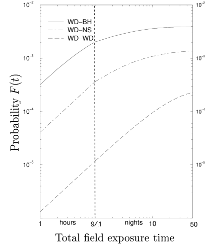
Figure 7: Probability $F(t)$ of detecting a flare with $\Delta m\geq 0\aas@@fstack{m}2$ as a function of the overall observation time of a specified sky region measured either in hours or in nights.

The values of $F(K_{0},t)$ for $K_{0}=1.2(\Delta m=0\aas@@fstack{m}2)$ and $t=9^{h}$ are presented in Table 4 for a range of $a_{0}$ and $a_{max}$ values. These rough model estimates may change by a factor of 1.5–2 depending on the real pattern of the distribution of pairs of compact objects along the semiaxes.

Table 4: Probabilities of detection of flares with $\Delta m=0\aas@@fstack{m}2$ in 9 hours

Parameters	WD + WD		WD + NS		WD + BH
$\quad(R_{\odot})$
$a_{0}\;\;\;\setminus\;\;\;a_{max}$	50	30	50	30	50	30
10	$1.4\cdot 10^{-5}$	$1.6\cdot 10^{-5}$	$1.7\cdot 10^{-4}$	$2.2\cdot 10^{-4}$	$9.8\cdot 10^{-4}$	$1.3\cdot 10^{-3}$
8	$1.3\cdot 10^{-5}$	$1.4\cdot 10^{-5}$	$2.2\cdot 10^{-4}$	$2.7\cdot 10^{-4}$	$1.2\cdot 10^{-3}$	$1.6\cdot 10^{-3}$
7	$1.2\cdot 10^{-5}$	$1.3\cdot 10^{-5}$	$2.4\cdot 10^{-4}$	$3.1\cdot 10^{-4}$	$1.4\cdot 10^{-3}$	$1.8\cdot 10^{-3}$
5.88	$1.1\cdot 10^{-5}$	$1.2\cdot 10^{-5}$	$3.0\cdot 10^{-4}$	$3.7\cdot 10^{-4}$	$1.6\cdot 10^{-3}$	$2.0\cdot 10^{-3}$
4	$9.9\cdot 10^{-6}$	$1.0\cdot 10^{-5}$	$4.2\cdot 10^{-4}$	$5.0\cdot 10^{-4}$	$2.2\cdot 10^{-3}$	$2.7\cdot 10^{-3}$
3	$9.1\cdot 10^{-6}$	$9.2\cdot 10^{-6}$	$4.9\cdot 10^{-4}$	$5.9\cdot 10^{-4}$	$2.6\cdot 10^{-3}$	$3.1\cdot 10^{-3}$
Average	$10^{-5}$		$4\cdot 10^{-4}$		$2\cdot 10^{-3}$
estimate

Fig.7 represents the behaviour of $F(t)\equiv F(K_{0},t)$ (for $\Delta m=0\aas@@fstack{m}2)$ as a function of $t$ and $n$ for the values of $a_{0}$ and $a_{max}$ which give approximately the average values among those presented in Table 4 for different system types.

We have also estimated the average durations and periods of reccurence of the events considered and their dispersions using (20) – ($22^{\prime}$). To do this correctly one has to convolve $\tau$ and $T$ not with the $f(a)$ but with the $P(K_{0},t,a)f(a)/F(K_{0},t)$ according to the share each parameter region brings to the probability of detecting a flare. These values, formally, depend on the values of $t$ or $n$. However, it is clear that their variations cannot influence much the real average characteristic. Actually in these calculations we use the expression for $P(K_{0},t,a)$ and $F(K_{0},t)$ in the region where they are linear in $t$, which as we will see in Section 5 corresponds to the optimal strategy for searching for the flares.

The results are presented in Table 5 for the value of amplitude $\Delta m\geq 0\aas@@fstack{m}2$. The parameters averaged over the range of the used $a_{0}$ (from $3R_{\odot}$ to $10R_{\odot}$) are in the first and third columns. Variations of flare duration with varying $a_{0}$ do not exceed a factor of 2. In columns 2 and 4 the limits of the intervals which contain parameters of 90 % of flares are given. The minimum values of the parameters correspond to the closest systems of all types which are capable of giving rise to a flare with the amplitude $\Delta m\geq 0\aas@@fstack{m}2$. In Table 5 we give parameters of events that one can hope to discover in observations.

4 The number of pairs being investigated in the Galaxy

As we have already noted, the present-day numbers of different pairs of compact objects are determined in the framework of different versions of population synthesis (Lipunov et al. 1996; Wellstein & Langer 1999; Fryer et al. 1999; Nelemans et al. 2001). However, the main objective of this research is the study of systems which are of interest within the scope of gravitational-wave astronomy and of the problem of origin of gamma-ray bursts. These are pairs of neutron stars, neutron stars with black holes and essentially rarely white dwarfs with black holes. By now extensive work has been done on the modeling of the origin and evolution of pairs of white dwarfs. It goes without saying that these binary systems are best understood; comparison with observations can be made for them (Hernanz et al. 1997; Nelemans et al. 2001). There are at least two relatively reliable estimates of the total number of binary white dwarfs in the Galaxy, $5\cdot 10^{8}$ (Lipunov et al. 1996) and $2.5\cdot 10^{8}$ (Nelemans et al. 2001). In principle, these data are sufficient to determine the number of gravitational-lens flares that can be detected in this sample. Nevertheless, we have estimated the number of binary white dwarfs and also white dwarfs in pairs with neutron stars and black holes in the Galaxy in the framework of assumptions of the progenitors of binary systems consisting of compact objects. We have followed Bethe and Brown (1998, 1999) who have determined the number of massive binaries containing neutron stars and black holes.

Table 5: Parameters of flares of amplitude $\Delta m\geq 0\aas@@fstack{m}2$

	Duration (s)		Period of recurrence (h)
	average	interval of	average	interval of
		90%		90%
WD+BH	50	10-135	15	1-48
WD+NS	60	20-120	42	8-120
WD+WD	135	90-180	400	120-500

We will base our discussion on the following assumptions (as previously, solar units are used).

1. The mass distribution of progenitor stars (initial mass function) obeys Salpeter’s (1955) law in the interval $0.1<M<120$, i.e.

$$dW(M)=w(M)dM=1.35(\frac{M}{0.1})^{-2.35}dM\;,$$ (23)

where $dW(M)$ is the probability that the mass of a star will be in the interval $M\div M+dM$, $w(M)$ is the probability density.

At the observed star formation rate $\frac{dN}{dM\cdot dt}=0.9(\frac{M}{0.1})^{-2.35}{\rm year}^{-1}$ and the Galaxy age of $10^{10}$ years, the number of stars is $N\sim 1.5\cdot 10^{11}$.

2. About 100 % of stars are members of binary systems. This evaluation is used in the population synthesis as well as 50 % (see for instance, Nelemans et al. 2001).

3. The distribution density in the mass ratio, $q\equiv M_{s}/M_{l}\leq 1$, is constant, i.e. $\frac{dN}{dq}\propto{\rm const}$ ( e.g. Portegies Zwart & Yungelson 1998).

4. The initial masses of progenitor stars must lie within the following intervals to give:
white dwarf – $1<M<10$, neutron star – $10<M<25$, black hole – $25<M$.
In the last case the uncertainty is rather great; the values $40M_{\odot}$ (Van den Heuvel & Habets 1984), and $60M_{\odot}$ (Woosly et al. 1995) are also used. As for us, we follow Portegies Zwart et al. (1997).

5. The neutron star formed in a supernova explosion in a binary system receives a kick. As Cordes & Chernoff (1997) have shown, its distribution is well approximated by the sum of two Gaussians with standard 175 km/s and 700 km/s, the share of the former being 80 % while that of the latter being 20 %. With these parameters 43 % of binary systems survive after the explosion (Bethe & Brown 1998). As a black hole is formed, one can believe that the kick will be lower, at least, inversely proportional to its mass (Fryer et al. 1999). For this case, using the relationships between the probability of decay and the additional velocity derived by Bethe & Brown (1998), we have found that 87 % of binaries survive after the formation of a black hole.

Now we turn to estimation of the number of pairs of different types.

For the probability $d\phi$ to obtain a binary system with the mass of the more massive companion (in our case the object is a lens) in the interval $M_{l}\div M_{l}+dM_{l}$ and the mass ratio in the interval $q\div q+dq$, considering (23) and the homogeneity of the distribution in $q$ ($M_{l}$ is measured in $0.1M_{\odot}$), we have

$$d\phi=dqdW=1.35(M_{l})^{-2.35}dqdM_{l}.$$ (24)

The number of pairs of type $i$ is $N_{i}=\phi_{i}\gamma_{i}N_{bin}$, $i=d$ for a pair of white dwarfs, $i=n$ and $i=b$ for binaries containing a white dwarf with a neutron star and a black hole, respectively; $\gamma_{i}$ is the pair survival probability after the supernova explosion.

Clearly

$$\phi_{i}=\int\limits_{Q_{i}}\int\limits_{M_{i}}d\phi=1.35\int\limits_{Q_{i}}\int\limits_{M_{i}}(M_{l})^{-2.35}dqdM_{l},$$ (25)

where $Q_{i}$ is the interval where the values of $q$ lie, and $M$ is the interval of $M_{l}$ values. Determine $Q_{i}$ for each type of pairs, taking into account that $10<M_{s}=qM_{l}<100$ (assumption 5). Then $\frac{10}{M_{l}}<q<1$ for a pair WD–WD, $\frac{10}{M_{l}}<q<\frac{100}{M_{l}}$ for a pair WD–NS and WD–BH. Thus, proceeding from (25), we obtain for a pair of white dwarfs

$$\begin{array}[]{ll}\phi_{d}&=1.35\int\limits_{10}^{100}(M_{l})^{-2.35}dM_{l}\int\limits_{\frac{10}{M_{l}}}^{1}dq\\ &=1.35\int\limits_{10}^{100}(M_{l})^{-2.35}\left(1-\frac{10}{M_{l}}\right)dM_{l}.\end{array}$$ (26)

Hence

$$\begin{array}[]{ll}\phi_{d}&=1.35\int\limits_{10}^{100}M_{l}^{-2.35}dM_{l}-13.35\int\limits_{10}^{100}M_{l}^{-3.35}dM_{l}\\ &=0.043-0.025=0.018,\end{array}$$

and allowing for the fact that the number of pairs in the Galaxy is $N_{bin}=0.5N$, obtain for the number of binary white dwarfs $N_{d}=1.35\cdot 10^{9}$ pairs.

For white dwarfs in pair with neutron stars

$$\begin{array}[]{ll}\phi_{n}&=1.35\int\limits_{100}^{250}M_{l}^{-2.35}dM_{l}\int\limits_{\frac{10}{M_{l}}}^{\frac{100}{M_{l}}}dq\\ &=1.35\int\limits_{100}^{250}M_{l}^{-2.35}\frac{90}{M_{l}}dM_{l}=90\cdot 1.35\int\limits_{100}^{250}M_{l}^{-3.35}dM_{l},\end{array}$$

and finally

$$\phi_{n}=\frac{90\cdot 1.35}{2.35}\left[M_{l}^{-2.35}\Bigr{|}_{100}^{250}\right]=51.7\cdot 1.76\cdot 10^{-5}=9.1\cdot 10^{-4}.$$

Because 57 % of binary systems decay after the supernova explosion which results in formation of a neutron star, $N_{n}\sim 9.1\cdot 10^{-4}\cdot 0.43\cdot 0.5N\sim 2.9\cdot 10^{7}$ pairs.

The same is for pairs containing black holes:

$$\phi_{b}=51.7\left[M_{l}^{-2.35}\Bigr{|}_{250}^{1200}\right]=51.7\cdot 2.26\cdot 10^{-6}=1.2\cdot 10^{-4}.$$

Since the probability of their survival is 87%, then $N_{b}\sim 1.2\cdot 10^{-4}\cdot 0.87\cdot 0.5\cdot N\sim 7.8\cdot 10^{6}$ pairs.

It should be emphasized that the above-given estimates are defined in many respects by the choice of the power index $k$ in the initial function of stellar masses. Clearly they decrease with increasing $k$. It is likely that the version with $k=2.35$ of Salpeter (1955) is most consistent with current observational data (see, for instance, Grishchuk et al. 2001; Raguzova 2001), but, nevertheless, $k=2.5$ and also $k=2.7$ are used in the population synthesis as well (Bethe & Brown 1998, 1999; Nelemans et al. 2001).

To make the picture complete, we present in Table 6 the estimates of the numbers of pairs in the Galaxy for the mentioned $k$.

Table 6: Estimates of the number of pairs of compact objects for different mass functions

$k$	WD–WD	WD–NS	WD–BH
2.35	$1.3\cdot 10^{9}$	$2.7\cdot 10^{7}$	$8\cdot 10^{6}$
2.5	$8.7\cdot 10^{8}$	$1.6\cdot 10^{7}$	$4\cdot 10^{6}$
2.7	$5.5\cdot 10^{8}$	$6\cdot 10^{6}$	$1.2\cdot 10^{6}$

On the other hand, in order to determine the accuracy of our estimates, one can compare them (for binary white dwarfs) with the results of population synthesis. In particular, the number of pairs of this type is $4.5\cdot 10^{8}$ (Lipunov et al. 1996) and $2.5\cdot 10^{8}$ (Nelemans et al. 2001). Note that the last number was obtained for $k=2.7$ and it is 2 times as low as our rough value from Table 6. The 2-4–time differences are reasonable, taking into account the uncertainty in the results of modeling of evolution and the qualitative character of our estimates.

5 Strategy of search and the number of detectable objects. Conclusions

To determine the number of objects that may be detected using a certain telescope one has to know not only the overall number but also their distribution in the Galaxy, their luminosity function and the distribution of absorbing matter as well.

We used the star distribution in the Galaxy of the following form:

$$\rho=\rho_{0}e^{-\frac{R}{H}}e^{-\frac{|z|}{h}},$$ (27)

where $R$ and $z$ are the point cylindrical coordinates in the Galaxy, $H$ and $h$ are radial and vertical distance scales, respectively, for which we used the following values: $H=8$ kpc and $h=250$ pc (see Dehnen & Binney 1998; Nelemans et al. 2001). Adopting the Sun’s coordinates $R_{\odot}=8.5$ kpc and $z_{\odot}=30$ pc we have:

$$\rho_{0}=\rho_{loc}e^{\frac{R_{\odot}}{H}}e^{\frac{z_{\odot}}{h}}.$$

The overall number of objects in the Galaxy is expressed by the integral

$$N=\int\limits_{-\infty}^{\infty}dz\int\limits_{0}^{\infty}2\pi R\rho_{0}e^{-\frac{R}{H}}e^{-\frac{|z|}{h}}dR,$$

which yields

$$\rho_{loc}=\frac{Ne^{-\frac{R_{\odot}}{H}}e^{\frac{|z_{\odot}|}{h}}}{4\pi H^{2}h}=\frac{N}{6.56\cdot 10^{11}}{\rm pc^{-3}}$$ (28)

and

$$\rho(R,z)=\frac{N}{6.56\cdot 10^{11}}e^{-\frac{R-R_{\odot}}{H}}e^{-\frac{|z|-z_{\odot}}{h}}{\rm pc^{-3}}.$$ (29)

We used distributions for WD-NS and WD-BH in the same form with the only difference in normalization coming from their fewer overall number in the Milky Way. The local densities corresponding to the overall numbers given in Table 6 are presented in Table 7.

Note that the part of WD-WD pairs among the complete number of WDs is (7-25) % (Iben et al. 1997; Fryer et al. 1999) and the WD density in the Solar neighbourhood is $(4-20)\cdot 10^{-3}$ pc^-3 (see Nelemans et al. 2001 and references therein). This gives us a range of local density of $3\cdot 10^{-4}-5\cdot 10^{-3}$ pc^-3. It is very close to our estimate shown in Table 7 and the most optimistic values of density may be $2-2.5$ times more than those.

Unfortunately, there is no data to compare with for binaries other than WD-WD. We suggest only that our estimation range may be $2-3$ times narrower. Therefore, the real number of objects may be a few times higher.

Table 7: The local densities of objects derived from Table 6 data and distirbution (27) (in pc^-3).

$k$	WD–WD	WD–NS	WD–BH
2.35	$2.0\cdot 10^{-3}$	$4.1\cdot 10^{-5}$	$1.2\cdot 10^{-5}$
2.5	$1.3\cdot 10^{-3}$	$2.4\cdot 10^{-5}$	$6.1\cdot 10^{-6}$
2.7	$8.4\cdot 10^{-4}$	$9.1\cdot 10^{-6}$	$1.8\cdot 10^{-6}$

The insterstellar absorption is proportional to the interstellar medium density which is distributed in the Galaxy by the same  (27) law with $h=80$ pc (Dehnen & Binney 1998). The normalization was done according to the local average value of absorption $A_{g^{\prime}}=1\aas@@fstack{m}16{\rm kpc^{-1}}$ in the $g^{\prime}$ band of the SDSS equipment (Schlegel et al. 1998).

The WD luminosity function is well known and is explained fairly well in the frame of their cooling theory. We used the luminosity function of Oswalt et al. (1996). It is readily seen from this that more than half of the WDs are brighter than $13\aas@@fstack{m}5$ and only less than 20 percent are fainter than $15^{\rm m}$, where the function reaches its maximum. Thus, the magnitudes of the majority of WDs do not suffer much from the bolometrical corrections which is a few tenth for the stars of these spectral classes (see, e.g. Allen 1973).

In other binary systems, the situation is more complicated. It is only clear that the optical emission from both a NS and a BH can be associated with interstellar gas accretion. In the former case it is likely to be negligibly small because of the high orbital velocity of the NS ($>100$ km/s) (Shapiro & Teukolsky 1983). At the same time the orbital velocity of a BH in a pair with a WD is about 50 km/s, and the luminosity of accretion plasma can reach $10^{30}$ erg/s by moderate-optimistic estimates (Shvartsman 1971; Beskin & Karpov 2002) and will be by an order of magnitude less by a pessimistic one (Ipser & Price 1982). Apparently, its contribution to the total luminosity of the system is insufficient to correct the depth of the space of detection. However, this level of optical emission makes possible searching for its fast variations with a microsecond time resolution for investigation of accretion processes and strong gravitational fields near the horizon of events (Shvartsman 1971; Beskin et al. 1997; Beskin & Karpov 2002).

Now we have everything we need to calculate the on-sky density of objects in a given direction ($l,b$):

$$\begin{array}[]{ll}\sigma(l,b)&=\frac{d^{2}N}{\cos{b}dldb}\\ &=\int r^{2}\rho(R,z)I(M)dr\;,\end{array}$$ (30)

where $I(M)$ is a cumulative luminosity function from Oswald et al. (1996), $M=m_{lim}-5\lg(r/10)-A(r,l,b$), $m_{lim}$ is an equipment limiting apparent stellar magnitude, $A(r,l,b)$ is a total extinction in the $(l,b)$ direction up to the distance $r$, and

$$\begin{array}[]{l}z=z_{\odot}+r\sin{b},\\ R=\sqrt{R^{2}_{\odot}+r^{2}\cos^{2}{l}-2R_{\odot}r\cos{b}\cos{l}}\end{array}$$

are the point cylindrical coordinates expressed in terms of its galactic coordinates $(l,b)$ and distance $r$.

Unfortunately, this integration cannot be done analytically and so we will turn at once to a particular version of the equipment being discussed. In our view, an ideal tool for carrying out the proposed programme is currently the 2.5-metre telescope at APO (New Mexico). It has been used to accomplish one of the most promising projects – the Sloan Digital Sky Survey (SDSS). The telescope has a field of $3^{\circ}$, in which 30 CCD chips of $2048\times 2048$ pixels are mounted (York et al. 2000). Sky scanning at a speed of its movement along a strip $2\aas@@fstack{\circ}5$ wide is performed within the framework of the project. During an exposure of 55 s, the limiting stellar magnitude in the $g^{\prime}$ filter (it is close to the $B$ filter of the Johnson system) is $23\aas@@fstack{m}2$ at a signal-to-noise ratio of $\sim 5$ (Oke & Gunn 1983; York et al. 2000). We have constructed a relationship between amplitude of flares recorded at a $5\sigma$ level and stellar magnitude of a quiet object in the $g^{\prime}$ band (Fig. 8). In so doing, we used the parameters corresponding to the SDSS project: the seeing – 0.8 arcsec, the quantum efficiency of the CCD matrix – 80 %.

By comparing the data of Fig. 8 with the mean parameters of flares (Table 5) and their light curves for different binary systems (Fig. 5), it is clear that with a particular exposure of time $t_{e}\sim 10-30$ s, the flares with $\Delta m\geq 0\aas@@fstack{m}2$ of any pairs that we have examined can be recorded at a significance level of $5\cdot 10^{-3}-10^{-5}$ (duration of any flare is a few $t_{e}$). In fact, the level of the flare detection will be better due to registration in the SDSS of the field in several colour bands ($u^{\prime},g^{\prime},r^{\prime},z^{\prime}$) and the limiting $r^{\prime}$ stellar magnitude is also $23\aas@@fstack{m}$ Moreover, the use and comparison of the data in the $g^{\prime}$ and $r^{\prime}$ filters give the possibility of easy separation of cosmic ray traces.

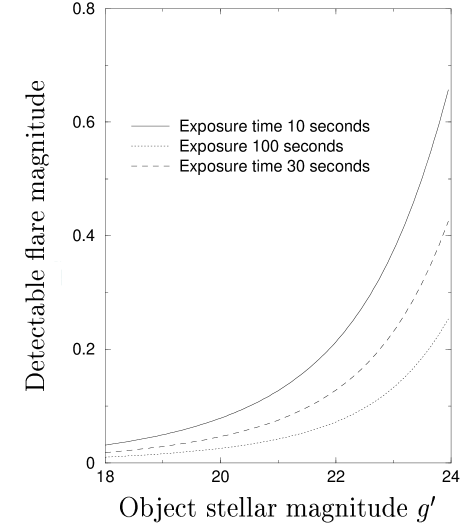
Figure 8: Magnitudes of detectable flares in the SDSS versus object brightness

On the basis of (30) we have built a map of the expected on-sky densities of WD-WD pairs up to $m_{lim}=23^{\rm m}$ which is presented in Fig. 9. The value of the local density corresponding to the Salpeter mass-spectrum index of $2.35$ is used. One can see from the map that the maximal density regions have galactic latitudes of $5-10$ degrees and a question might arise if it is possible to observe in such star-rich regions of the sky. However, even in these latitudes the average distance between stars of up to $23^{\rm m}$ is about 3-4 arcseconds (see e.g., Zombeck, 1982, p.34) and thus, they are resolved with the SDSS seeing and this crowding therefore cannot have much negative impact on observations with this equipment.

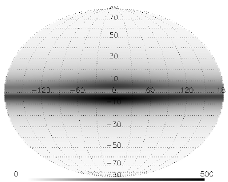
Figure 9: Simulated on-sky distribution of WD-WD pairs, $m_{lim}=23^{\rm m}$. Maximum density value is 490 pairs per square degree.

To derive the expected number of events of the discussed type $N_{exp}$ one multiplies the probability of detecting it from a randomly chosen pair $F(t)$ for $\Delta m=0\aas@@fstack{m}2$ (see (15), (20)-(22^′) and Fig.7) by the number $D(\Omega)$ of such pairs observed during a certain observational programme that covered the celestial sphere part $\Omega$:

$$N_{exp}=F(t)\times D(\Omega),$$ (31)

where

$$D(\Omega)=\int\limits_{\Omega}\sigma(l,b)\cos{b}dldb\;.$$ (32)

It is clear, however, that when applying to reality one deals with a telescope of limited field of view and the observational time provided for a programme is limited as well, so increasing the total exposure of a field to increase $F(t)$ leads to decreasing the number of such fields in the programme. It is also evident that one has to monitor at first the best, i.e. maximal density $\sigma(l,b)$ fields first. Fig. 10 represents the number of pairs of each type $D(\Omega)$, numerically calculated from (32), in $\Omega$ fields with a size of $2\aas@@fstack{\circ}5\times 2\aas@@fstack{\circ}5$ (field of view of SDSS) after sorting them in decending order of pair density.

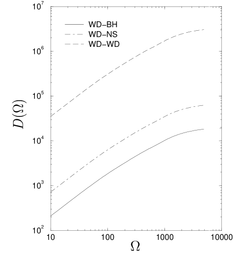
Figure 10: Expected number of objects $D(\Omega)$ in $\Omega$ the best (with the highest density of pairs) $2\aas@@fstack{\circ}5\times 2\aas@@fstack{\circ}5$ fields.

Now let the programme last for 5 years. Considering that the matter in question is detection of rather faint objects, observations have to be made on dark nights only at moon phases within $\pm 5^{d}$ from the new moon, which gives approximately $36\%$ of night time. Assuming the average observational night of $9^{h}$ the 5-year resource of time then will make $n_{obs}=657$ nights or $T_{obs}=5913$ hours. Thus, as every field is observed for $t$ hours or $n$ nights (and $\Omega=T_{obs}/t$, $n_{obs}/n$) the expected number of detected pairs is

$$N_{exp}=D\left(\frac{T_{obs}}{t}\right)F(t),$$ (33)

or

$$N_{exp}=D\left(\frac{n_{obs}}{n}\right)F(n).\hskip 130.88284pt(33^{\prime})$$

These quantities derived from Figs. 7 and 10 are presented in Fig. 11. One can see from this figure that the optimal total exposure per field for WD-WD pairs is $6-7$ nights, and it is about 1 night when searching for WD-NS or WD-BH systems.

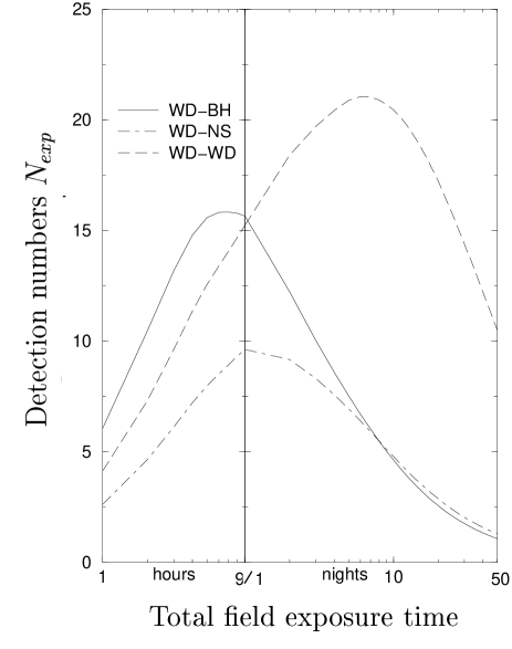
Figure 11: Expected detection numbers in the 5-year programme as a function of total exposure per field.

The expected numbers of detections with optimal strategies along with the optimal total exposures per field are given at Table 8.

Table 8: The number of pairs of compact objects detectable over 5 years and the optimal total exposures per field

$k$	WD–WD	WD–NS	WD–BH
2.35	22	9	16
2.5	15	5	8
2.7	9	2	3
Optimal
exposure time	6-7 nights	1-2 nights	6-9 hours
per $2\aas@@fstack{\circ}5\times 2\aas@@fstack{\circ}5$ field

A new project entitled ”The Dark Matter Telescope” (http://www.dmtelescope.org/index.htm) being developed involved 8.4 (effectively 6.9) metre telescope with a field of view slightly wider than that of the SDSS. The use of it in a manner similar to that described above increases the number of detectable objects by a factor of 2.2. Other wide field telescopes of 4 metres in diameter being built now, LAMOST (http://www.greenwich-observatory.co.uk/lamost.
html) and VISTA (http://www.vista.ac.uk), could detect 1.5 times more binaries than the SDSS.

Thus, for searching for the flares caused by gravitation lensing in binary systems with compact companions, the facilities of the SDSS can be used, having reduced the time of an individual exposure to 10-20 s. It is obvious that after recording a flare in a certain object, another telescope of similar class must be involved in observations. This object should be monitored to prove the effect and for detailed investigation of the detected system.

Thus, within the frame of the proposed programme, it will be possible to find several dozen binary systems comprised of compact objects. It will be recalled that in numerous surveys of microlensing, the number of reliably detected events amounts to about 350 (Alcock 1999), only in two cases the matter in question being of massive lenses (black holes?) (Bennett et al. 2001). When applying the technique suggested, there is a possibility of detecting with absolute assurance more than 10 black holes with open event horizons. An investigation of these objects with high time resolution within the MANIA experiment (Beskin et al. 1997) may permit at last the detection of observational evidence of extreme gravitational fields.

- (1) Abt, H.A. 1983, ARA&A, 21, 343
- (2) Agol, E. 2002, astro-ph/0207228
- (3) Alcock, C. 1999, BAAS, 31, 1554
- (4) Allen, C.W. 1973, Astrophysical quantities (London: The Athlone Press)
- (5) Bennett, D.P., Becker, A.C., Quinn, J.L., et al. 2001, astro-ph/0109467
- (6) Bethe, H.A., & Brown, G.E. 1998, ApJ, 506, 780
- (7) Bethe, H.A., & Brown, G.E. 1999, ApJ, 517, 318
- (8) Beskin, G., Komarova, V., Neizvestny, S., et al. 1997, Experimental Astronomy, 7, 413
- (9) Beskin, G., & Karpov, S. 2002, Gravitation & Cosmology Suppl. Ser., 8, 182
- (10) Byalko, A.V. 1969, SvA, 46, 998
- (11) Cherepashchuk, A.M., & Bogdanov, B.M. 1995a, SvA, 72, 873
- (12) Cherepashchuk, A.M., & Bogdanov, B.M. 1995b, SvAL, 21, 8, 570
- (13) Cherepashchuk, A.M. 2001, UFN, 171, 864
- (14) Cordes, J.M.,& Chernoff, D.F. 1997, ApJ, 482, 971
- (15) Damour, T. 2000, NPhB, 80, 41
- (16) Dehnen, W., & Binney, J.J. 1998, MNRAS, 298, 387
- (17) Fryer, C.L., Woosley, S.E., & Hartmann, D.H. 1999, ApJ, 526, 152
- (18) Goncharsky, A.V., Cherepashchuk, A.M., & Yagola, A.G. 1985, Singular problems of astrophysics (Moscow: Nauka)
- (19) Gould, A. 1995, ApJ, 446, 541
- (20) Grishchuk, L.P., Lipunov, B.M., Postnov, K.A., et. al. 2001, UFN, 171, 3
- (21) Hernanz, M., Isern, J., & Salaris, M. 1997, in Proceedings of the 10th European Workshop on White Dwarfs, eds. J. Isern, M. Hernanz, E. Gracio-Berro, 214, 307
- (22) Iben, I.Jr., & Tutukov, A.V. 1984, ApJS, 54, 355
- (23) Iben, I.Jr., Tutukov, A.V., & Yungelson, L.P. 1997, ApJ, 475, 268
- (24) Ingel, L.H. 1972, SvA, 150, 1331
- (25) Ingel, L.H. 1974, Astrophizika, 10, 555
- (26) Ipser, J.R., & Price, R.H. 1982, ApJ, 255, 654
- (27) Landau, L.D., & Livshits, E.M. 1983, Theory of field (Moscow: Nauka)
- (28) Liebert, J., Dahn, C.C., & Monet, D.G. 1988, ApJ, 332, 891
- (29) Liebes S. 1964, Phys. Rev., 133, 835
- (30) Lipunov, V.M., Postnov, K.A., & Prokhorov, M.E. 1996, The Scenario machine: Binary star population synthesis (Amsterdam: Harwood Academic Publishers)
- (31) Maeder A. 1973, A&A, 26, 215
- (32) Marsh, T.R. 2001, MNRAS, 324, 547
- (33) McCook, G.P., & Sion, E.M. 1987, ApJS, 65, 603
- (34) Masevich, A., & Tutukov, A. 1988, Stellar evolution (Moscow: Nauka)
- (35) Maxted, P.F.L., Marsh, T.R., Moran, C.K.J., & Han, Z. 2000, MNRAS, 314, 334
- (36) Nauenberg, M. 1972, ApJ, 175, 417
- (37) Nelemans, G., Yungelson, L.R., Portegies Zwart, S.F., & Verbunt, F. 2001, A&A, 365, 491
- (38) Oke, J.B., & Gunn, J.E. 1983, ApJ, 266, 713
- (39) Oswalt, T.D., Smith, J.A., Wood, M.A., & Hintzen, P. 1996, Nature, 382, 692
- (40) Portegies Zwart, S.F., Verbunt, F., & Ergma, E. 1997, A&A, 321, 207
- (41) Portegies Zwart, S.F., & Yungelson, L.P. 1998, A&A, 332, 173
- (42) Qin, B., Wu, X.-P., & Zou, Zh. 1997, Chin. Phys. Lett., 14, 155
- (43) Raguzova, N.V. 2001, A&A, 367, 848
- (44) Refsdal, S. 1964, MNRAS, 128, 295
- (45) Saffer, R.A., Livio, M., & Yungelson, L.R. 1998, ApJ, 502, 394
- (46) Salpeter, E.E. 1995, ApJ, 121, 161
- (47) Savage, B.D., & Mathis, J.S. 1979, ARA&A, 17, 73
- (48) Schlegel, D.J., Finkenbeiner, D.P., & Davis, M. 1998, ApJ, 500, 525
- (49) Shapiro, S., & Teukolsky, S. 1983, Black Holes, White Dwarfs and Neutron Stars (New York: A Wiley-Interscience Publication)
- (50) Shvartsman, V.F. 1971, SvA, 48, 3
- (51) Van den Heuvel, E.P.J., & Habets, G.M.H.J. 1984, Nature, 309, 598
- (52) Thorsett, S.E., & Chakrabarty, D. 1999, ApJ, 512, 288
- (53) Webbink, R.F. 1984, ApJ, 277, 355
- (54) Wellstein, S., & Langer, N. 1999, A&A, 350, 148
- (55) Woosly, S.E., Langer, N., & Weaver, T.A. 1995, ApJ, 448, 315
- (56) Yakovlev, D.G., Levenfish, K.P., & Shibanov, Yu.A. 1999, UFN, 169, 825
- (57) York, D.G., Donaild, G., Adelman, J., et al. 2000, AJ, 120, 1579
- (58) Yungelson, L.R., Livio, M., Tutukov, A.V.,& Saffer, R.A. 1994, ApJ, 420, 334
- (59) Zakharov, A. 1997, Gravitational lenses and microlenses (Moscow: Yanus)
- (60) Zakharov, A., & Sazhin, M. 1998, UFN, 168, 1041
- (61) Zombeck, M.V. 1982, Handbook of Space Astronomy and Astrophysics (Cambridge: Cambridge University Press)