The Internal Extinction Curve of NGC 6302 and its Extraordinary Spectrum

Abstract

In this paper we present a new method for obtaining the optical wavelength-dependent reddening function of planetary nebulae, using the nebular and stellar continuum. The data used was a spectrum of NGC 6302 obtained using the Double Beam Spectrograph on the 2.3m telescope at Siding Springs Observatory over three nights. This resulted in a spectrum covering a wavelength range $3300-8600$ Å  with a large dynamical range and a mean signal to noise of $>10^{2}$ Å^-1 in the nebular continuum. With such a high S/N the continuum can be accurately compared with a theoretical model nebular plus stellar continuum. The nebular electron temperature and density used in the model are determined using ratios of prominent emission lines. The reddening function can then be obtained from the ratio of the theoretical and the observed continuum. In the case of NGC 6302, it is known that much of the reddening arises from dust within or around the nebula, so that any differences between the measured reddening law and the ‘standard’ interstellar reddening law will reflect differences in the nebular grain size distribution or composition. We find that for NGC 6302, the visible to IR extinction law is indistinguishable from ‘standard’ interstellar reddening, but that the UV extinction curve is much steeper than normal, suggesting that more small dust grains had been ejected into the nebula by the PN central star. We have detected the continuum from the central star and determined its Zanstra Temperature to be of order 150,000K. Finally, using the extinction law that we have determined, we present a complete de–reddened line list of nearly 600 emission lines, and report on the detection of the He(2-10) and He(2-8) Raman Features at $\lambda 4331$ Å and $\lambda 4852$ Å, and the detection of Raman-Scattered O vifeatures at 6830 and 7087 Å. We believe this to be the first detection of this process in a PN.

¹ Research School of Astronomy and Astrophysics, Australian National University, Cotter Rd, Weston, ACT 2611, Australia
bgroves@mso.anu.edu.au, Michael.Dopita@anu.edu.au
² Space Telescope Science Institute,3700 San Martin Drive, Baltimore, MD, 21218, USA
wms@stsci.edu
³ Laboratorie d’Astronomie Spatiale, Marseille, France
Trung.Hua@astrsp-mrs.fr

Keywords: planetary nebulae: individual (NGC 6302) — ISM: dust, extinction

1 Introduction

Because interstellar dust grains are very small, typically less than a micron in diameter, their absorption and scattering properties are not only composition–dependent but also wavelength–dependent. Blue and UV light is usually preferentially scattered compared to that of longer wavelengths. Dust grains can not only absorb and scatter light from objects, they can also re-emit in the thermal infra-red, polarize light through grain alignment mechanisms or be accelerated, heated and photoelectrically charged by the electromagnetic radiation which impinges upon them.

All of these processes are known to occur in the planetary nebula (PN) environment. In particular, during the Asymptotic Giant Branch (AGB) phase of evolution, mass–loss releases material into the circum–stellar environment which has undergone partial nuclear processing in the central star. Since this environment is fairly cool, dust may be formed by direct condensation out of the gaseous phase whenever the kinetic temperature of the gas falls below a critical value which allows solids to form. In this case, we have a gas which is slowly cooling from higher temperatures and in which the pressure and supersaturation are high enough to allow both nucleation and grain growth. However, it is unlikely that there exists a state of thermodynamic equilibrium in the dust-forming gas, and shock heating and cooling are often both important. Therefore, a complex and detailed time-dependent description of the chemical reactions, usually referred to as a kinetic model, is needed to describe this situation.

Because of the physics of the condensation process, and the interaction between the grains formed in the flow and the radiation field of the star, there is a complex relationship between the nature of the grains, their size distribution and the terminal velocity of the dusty outflow. Kozasa & Sogawa (1997) showed that the grain size increases as the mass–loss rate increases, since the size of the grain produced by condensation depends upon the gas density in the wind where a strong supersaturation exists in the gaseous phase and upon the period during which the condensation timescale is much shorter than the dynamical expansion timescale. On the other hand, radiation pressure acting upon the grains accelerates the stellar mass-loss flow (thereby arresting the condensation process). This has been seen observationally by Loup et al. (1993) and explained theoretically by Habing et al. (1994). The expansion velocities of the carbon rich objects are larger than those of the oxygen rich AGB stars, and radiation pressure induced expansion of the atmosphere may limit the size of the typical carbon-bearing grain to $\sim 50$ Å, similar to that which is needed to explain the 2175 Å bump in the interstellar extinction curve. During the PN phase of evolution, we expect the grain size distribution to be further modified by radiative destruction processes (photoevaporation and coulomb destruction by excessive photoelectric charging) and by mechanical processes (grain coagulation and shattering).

Taking all of these considerations into account, it is clear that we should expect that the dust formed in the gas ejected during the AGB, and later observed in PN phase, would be quite unlike like that seen in the interstellar medium as a whole. It is therefore of great interest to either observe this dust directly through IR observations, or else through the extinction produced by it in the optical and UV.

As far as direct observations are concerned, enormous progress has recently been made using the ISO satellite to obtain spectroscopy of the far–IR emission features characteristic of different grain materials (Waters et al. 1996). The bright southern PN NGC 6302 is an ideal object for such studies, as it is known to have within it a dense circumstellar torus containing the bulk of the dust mass (Lester & Dinerstein, 1984), and within this, a dense ring of ionised gas, inclined at about 45 degrees to the plane of the sky (Rodriguez et al. 1985). Recently, Kemper et al. 2002 have reported the detection of features in the far–IR spectrum of this object which may be ascribed to the silicates amorphous olivine, forsterite, clino-enstatite, and diopside. In addition features due to water ice and metallic iron are seen. Remarkably, the carbonates calcite and dolomite were also detected.

At optical wavelengths, the lack of strong spectral features renders such exquisite mineralogy impossible. However, because dust grain dimensions are often comparable to or smaller than the wavelength of light, the dust extinction curve can in principle be used as a powerful constraint on the grain size distribution in the nebula.

For PNe we usually characterise the reddening by a single ‘reddening constant’, $c$, and then assume that the absorption through the optical wavelength region can be fit by a ‘standard’ Whitford (1958) reddening law. This curve, f($\lambda$), can then be used to deredden the observed emission line fluxes. The relationship between the corrected flux, F_c, and that observed, F_o is:

$$\text{F}_{c}=\text{F}_{o}\times 10^{cf(\lambda)}$$ (1)

The reddening constant is usually determined from a comparison of the ratio of the intensities of the Balmer lines, since this ‘Balmer decrement’ is only slightly dependent upon the temperature and density of the nebula, and the theoretical values are well–determined. Alternatively, we can compare the radio continuum flux density and the H$\beta$ flux. The radio emission is basically free from interstellar reddening and the ratio between the radio continuum flux and the H$\beta$ flux is determined only by the electron temperature and the relative helium abundance. A third technique is to measure the ratio of two emission lines which share a common upper energy level, such as H$\beta$ and Br$\gamma$ (Ashley, 1990).

All of these methods have their problems. In the first case, the reddening is determined at only a few discrete wavelengths, and over a restricted wavelength range. In the other two cases, we may be seeing regions of ionized gas in the radio or at IR wavelengths which are entirely dust–obscured in the optical, and therefore we can neither correctly evaluate the effective total obscuration nor the differential extinction at different optical wavelengths in the nebular gas.

The motivation behind the work described in this paper, is to obtain an intrinsic reddening function which does not depend on the Whitford curve, which is continuous in its wavelength coverage, and which can be used to place constraints on the grain size distribution in a planetary nebula.

To do this, we have obtained very high signal to noise observations of NGC 6302 covering the wavelength range $3300--8600$ Å, allowing observations of both Paschen and Balmer lines, and of both the Balmer and the Paschen discontinuities of Hydrogen. We have then compared the observed continuum spectral energy distribution to a theoretical (nebular $+$ stellar) spectral energy template to derive the reddening function. As far as we are aware, this represents the first practical application of this novel technique in the literature.

2 Observations and Reduction

NGC 6302 is a very bright, nearby Type I planetary nebula which displays a bipolar, filamentary structure. Its central star of the nebula is believed to be very hot, with a temperature possibly as great as 430000 K (Ashley & Hyland, 1988). However, the central star has never been identified either owing to heavy obscuration in the central parts of the nebula, or else owing to its extreme temperature.

To observe NGC 6302 we used the Double Beam Spectrograph (DBS) (Rodgers, Conroy & Bloxham 1988) with its EEV CCD detectors on the 2.3m telescope Siding Springs Observatory. A 1200 l/mm grating was used in both the red and the blue arms giving a wavelength coverage of just over 1000 Å. We observed NGC 6302 over three photometric nights (6–8 July 1999) in 6 independent wavelength ranges, corresponding to three grating settings per arm. These settings, given below, were chosen to allow a slight overlap between each spectrum, and to avoid placing strong emission lines in the overlap region:

1	3300-4300 (B)	5800-6800 (R)	Dichroic # 1
2	4200-5200 (B)	6700-7700 (R)	Dichroic # 5
3	5100-6100 (B)	7600-8600 (R)	Dichroic # 5

Dichroic filter #1 is the only one with satisfactory performance in the UV below the Balmer Discontinuity, but for the second and third grating setups, Dichroic #5 was used, since this gives smoother transmission characteristics in the red.

In order to obtain spectra of great dynamical range, we had to make a series of exposures of different lengths to ensure that we had good relative photometry for the bright emission lines such as the [O iii] $\lambda 5007$ line, which were saturated on the detector in the longer exposures. Three independent frames were taken for each exposure time to eliminate cosmic ray events and to reduce the noise in the final spectrum. The full set of exposures for each pair of grating settings were: 1) 20s, 60s, 200s, 500s, and 1500s; 2) 20s, 60s, 180s, 600s, and 1500s; 3) 500s, and 1500s. Only two exposures were required at the third setting because of the lack of strong emission lines in these two regions. Each spectrum was 1850 pixels in length and covered 200 spatial pixels, each corresponding to 0.91 arc sec. on the sky.

The slit width was chosen to be 2 arc sec. This optimises the throughput without appreciable degradation of the spectral resolution. The slit was placed on the brightest optical region of NGC 6302 as shown in Fig. 1. This image was obtained using the 2.3m imager, and is a colour composite of three observations through narrow-band filters isolating respectively: blue, [O iii] $\lambda 5007$ ; green, H $\alpha$, and red, [N II] $\lambda 6584$.

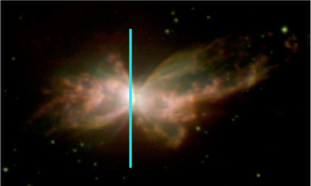
Figure 1: The planetary nebula NGC 6302 (Hua, Dopita & Martinis 1997). The placement of the 2.3m slit on the nebula is indicated by the blue line.

For wavelength calibration a Neon–Argon arc lamp was used, and for flux calibration the standard stars EG131 and Feige110 (Bessell, 1999) were observed. The star EG131 is particularly useful, because it lies not too far away on the sky from NGC 6302, and can therefore be used as an atmospheric standard as well. The flat field was generated by observing through the spectrograph, the diffuse reflection on a white-painted region of the shutter of the dome of an array of quartz-iodide lamps placed around the upper secondary support ring structure of the telescope.

The reduction of the data was done using the IRAF package. The reduction procedure was fairly complex, because of the number of observations, and the large dynamical range targeted for the final spectrum.

For each frame, the bias observed for that particular night was removed. However, as the telescope tracks, the spectrograph which is mounted at the Nasmyth A focus rotates, and consequently there is a temperature shift in the pre-amplification and CCD control electronics rack which is mounted on the spectrograph. This results in a systematic bias drift, which has to be removed in each frame by reference to the bias strip using the tasks IMSTAT and IMARITH. The spectrograph rotation also produces flexure which results in a small shift of the spectrum. To eliminate this, each set of three spectra were aligned relative to the observation that was nearest the arc observation using the IRAF task IMALIGN) and then combined using the IMCOMBINE option with the CCDREJECT option to remove cosmic ray events.

Flat fields were prepared by dividing each flat field observation by a low-order spline surface fit to the flat field to remove (to first order) the gross effects due to the spectral energy distribution of the quartz iodide lamps. At the UV end of the spectrum, around $3500-3300$Å, the accuracy of the flat field is limited by the photon statistics in the lamp. The flat fielding removes not only the point–like defects due to dust and blemishes in the CCD, but also the oscillations in the transmission of the dichroic beam–splitters, which is particularly noticeable in the red arm, close to the cutoff wavelength.

Following this, one dimensional spectra are extracted from a $\sim 6$ arc sec. length of slit centred on the eastern hot-spot. From this point, the data reduction follows the standard procedures described in the IRAF handbooks. The standard stars are also used as atmospheric standards to correct, as best as possible, for the OH atmospheric molecular band absorptions in the red.

After reduction, there remain a number of minor but significant problems in the data. First, the $4200-5200$Å observation suffers from grossly out of focus ghost images (produced in the camera) of the very bright [O iii] $\lambda\lambda 4959,5007$Å lines. These cannot be fully removed from the data, and corrupt the continuum measurements in the $\sim 4300-4600$Åwavelength range. In addition, the [O iii] lines themselves were so intense that in the long exposures, not only were the CCD columns containing these lines completely saturated, but there was also appreciable bleeding in the line direction as as well, up to the boundary of the chip near $5300$Å. An attempt has been made to correct for this effect, but the continuum fluxes measured in this spectral range remain less reliable.

Second, the absolute fluxes measured in the individual spectra differed from night to night, as judged from the overlap regions. This is probably mainly due to small errors in the re–positioning of the slit, despite the fact that the same centering and guide star offset figures were used for all three nights. Since the first night’s observations cover H$\alpha$ in the red, and H$\delta$ and beyond, down to the Balmer continuum in the blue, the remaining spectra were normalised by a fixed multiplicative factor to best remove any discontinuities in the overlap region.

Lastly, spectrograph drifts due to differential flexure problems during the long exposures provide a larger uncertainty in the absolute wavelength calibration than is desirable, with errors ranging up to $0.6$Å. However, the absolute wavelength scale is generally very accurately determined, with an error as small as $\sim 0.03$Å. However, in some cases, the lack of arc lines in the overlap region sometimes means that the systematic wavelength error in these regions may increase to up to $0.6$Å. Thus, the absolute wavelengths of individual spectral features should only be measured relative to nearby known hydrogen or helium lines, observed at the same time as the feature of interest.

In the long exposure (4500s integration time) combined spectrum, several of the bright lines were saturated on the CCD, sometimes quite grossly. The regions of saturation were determined, and the flux in these over–exposed regions was replaced by that measured in a shorter exposure in which these lines were not saturated. This gives a full spectrum which has a large wavelength range, high resolution, large S/N ratio and a very large dynamic range, shown in Fig. 2. Typically the mean signal to noise in the nebular continuum is $>10^{2}$ Å^-1. Hundreds of emission lines are visible. The identifications ascribed to these, and their relative intensities are discussed below. Note the prominent Balmer and Paschen discontinuities in the nebular continuum.

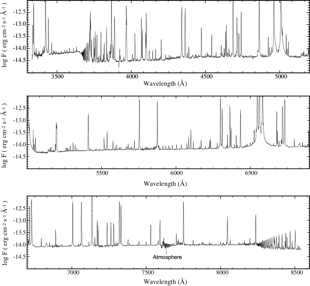
Figure 2: The spectrum of NGC 6302 covering a wavelength range of 3300–8600 Å and a very large dynamic range. Also visible in the spectrum is the nebular continuum, with a typical S/N greater than$10^{2}$ Å^-1. A full line list from this spectrum is given in in Table 3.

3 The Theoretical Nebular Continuum

The continuum emission from a planetary nebula comes from several processes. Given the temperature and density of the nebula and abundance of the emitting species, the full continuum emission from the nebula can be theoretically predicted. In the theoretical continuum emission calculated here the three main nebular emission processes were taken into consideration: free–free emission, free–bound emission and the two–photon continuum. The two major elements, Hydrogen and Helium were the only species considered as contributing to these processes. The theory of these processes, along with useful tables, is summarised by Dopita & Sutherland (2002).

For the first two processes, a simplified fit to the theoretical continuum emission due to Hydrogen and the two ionic states of Helium has been calculated from (Brown & Mathews 1970), which is applicable over the range of temperatures liable to be encountered. We fit the peaks of emission coefficient near prominent discontinuities (such as at the Balmer jump) with functions of the form:

$$\gamma_{\nu}\propto\text{T}^{\alpha}(1+\beta[\text{ln(T})]^{2})$$ (2)

with the constants $\alpha$ and $\beta$ and the constant of proportionality determined from the data for each peak.

Between discontinuities we fit the gradient of log$(\gamma_{\nu})$ vs. $\nu$ with a power law:

$$\text{gradient}\propto\text{T}^{\alpha}$$ (3)

with the constants $\alpha$ and the constant of proportionality determined from the data for each wavelength regions between peaks.

To these we add the theoretical emission from the two-photon process. The usual assumption, that there is a large optical depth for Ly$\alpha$ was adopted. Finally, the possibility that there is a continuum due to the central star should also be allowed for in making a fit to the observed nebular continuum. Here, we simply assume that since the central star is so hot, the spectrum can be fit by the Rayleigh–Jeans approximation for a Black Body.

The nebular continuum is normalised to the emissivity of H$\beta$ which can be obtained from Osterbrock (1989) or, equivalently from the tables in the appendices of Dopita & Sutherland (2002).

In order to fit this model continuum to the observed data, we need to observationally determine the parameters of nebular temperature, nebular density, and abundances by number of the He⁺ and He⁺⁺ ions relative to the H⁺ ion. These can be obtained with sufficient accuracy from the normal nebular diagnostics, provided that an initial estimate of the reddening can be determined, as shown in the following section.

4 Determination of Nebular Properties

There are a number of density sensitive line ratios available in the spectrum. These include the usual [O ii] $\lambda 3726/\lambda 3729$ and [S ii] $\lambda 6731/\lambda 6717$ line ratios, as well as the [Ar iv] $\lambda 4740/\lambda 4711$ and [Cl iii] $\lambda 5537/\lambda 5517$ line ratios which are not as frequently used because the lines are fainter, and their use requires spectra of higher signal to noise. Since all these lines pairs are close in wavelength, we do not have to worry about reddening corrections. The densities have been obtained from these ratios using the Australian version of the MAPPINGS III code (Sutherland & Dopita, 1993). The derived densities are listed in Table 1.

Line Ratio	Density ($10^{4}\rm{cm}^{-3}$)
[O ii]$\lambda 3726/\lambda 3729$	0.5
[S ii]$\lambda 6731/\lambda 6717$	0.8
[Ar iv]$\lambda 4740/\lambda 4711$	1.3
[Cl iii]$\lambda 5537/\lambda 5517$	2.0

Table 1: The measured electron density for NGC 6302 from several line ratios

In order to estimate the nebular temperature from line ratios, we first need to adopt an estimate of reddening. This was done as a first approximation by measuring the Balmer Decrement and comparing with the theoretical decrement for an assumed electron temperature of 15,000K (the choice of the electron temperature is not critical, since the Balmer decrement is little dependent on the temperature). Individual line ratios can then be dereddened using the Whitford reddening curve (as tabulated by Kaler, 1976). We find a reddening constant of $c=1.2$, in excellent agreement with that determined in the same way by Aller et al. 1981. They found $c=1.22$. It is interesting to note that these reddening values are lower than that obtained either from the H$\beta$ to Br$\gamma$ ratio ($c=2.44$, Ashley, 1990), or the H$\beta$ to radio continuum ratio ($c=2.1$, Milne & Aller, 1985; $c=2.1$, Ashley & Hyland, 1988). This is clear evidence that there exists a highly–obscured inner region in the nebula, visible only in the IR or at radio wavelengths.

The temperature sensitive lines used were [O iii] $\lambda 4363/\lambda 5007$, [N ii] $\lambda 5754/\lambda 6583$, [S ii] $\lambda 4076/\lambda 6731$ and [O i] $\lambda 5577/\lambda 6300$. The temperatures obtained from these ratios are listed in Table 2. Since the emission is heavily weighted towards the high–excitation regions in our spectrum, we adopt a temperature of $\text{T}_{e}\sim 1.5\times 10^{4}K$ for the continuum model fitting described below.

Line Ratio	Temperature ($10^{4}\rm{K}$)
[O iii]$\lambda 4363/\lambda 5007$	1.5
[N ii]$\lambda 5754/\lambda 6583$	1.4
[S ii]$\lambda 4076/\lambda 6731$	1.2
[O i]$\lambda 5577/\lambda 6300$	1.0

Table 2: The measured electron temperature for NGC 6302 from several line ratios

To determine the helium ionic abundance, ratios between the Pickering (n-4) and (n-3) lines and the Balmer lines for He ii and singlet lines such as $\lambda 6678$ and the Balmer lines for He i were used. We use the singlets for this purpose because, unlike the triplets, they are unaffected by optical depth and line transfer problems. The flux ratios are then be used with the data from Osterbrock (1989) and from Dopita & Sutherland (2002) to obtain the abundance of the He⁺ and He⁺⁺ions relative to H⁺.

The final parameters used in the calculation of the continuum are, temperature, $\text{T}_{e}\sim 1.5\times 10^{4}$ K, electron density, $\text{n}_{e}\sim 1.0\times 10^{4}$ cm^-3, He⁺ to H⁺ abundance ratio $\sim 0.11$ and He⁺⁺ to H⁺ abundance ratio $\sim 0.07$.

5 The Reddening Curve for NGC 6302

With the electron density, temperature and helium ionic abundances estimated above, we first built a theoretical continuum of NGC 6302, as shown in Fig. 3. This theoretical emission was then divided by the spectrum from NGC 6302 to provide an initial estimate of the reddening function. The result can be seen in Fig. 4. The reddening function should be a smooth curve which is defined by the highest points in this function. The detailed structure is due to the individual emission lines. However, even ignoring these emission line features, large steps are evident at both the Balmer and Paschen jumps. These steps would not be removed even were we to assume a much larger electron temperature, and in any case the residual Balmer and the Paschen jumps cannot both be simultaneously removed for any assumed value of the electron temperature.

We are forced to conclude that these discrepancies are the result of the presence of a reflected and/or direct continuum from the hot central star as discussed in §3, producing a Rayleigh–Jeans tail of a blackbody spectrum spectrum in the visible ($F_{\lambda}\propto\lambda^{-4}$).

Figure 3: The theoretical continuum of NGC 6302 relative to H$\beta$

Figure 4: The theoretical continuum divided by the spectrum of NGC 6302 showing the need for addition of a stellar continuum. The emission lines in the spectrum are responsible for the low values in this curve. The apparent features in the continuum between 4300 and 5200 Åare artifacts of the saturation effects and ghost images of the [O iii] lines described in section 2 and should be ignored.

The amount of stellar continuum which we need to add to match the observed Balmer jump determines the correct scaling factor of this Black–Body component to add to the continuum template. The correctness of this scaling factor is evidenced by the fact that, when this is done, the other jumps such as the Paschen and HeII jumps also match the observations. The resultant continuum model including the stellar contribution is shown in Fig. 5 and the result of division of this by the observational data is shown in Fig. 6.

This represents the first direct detection of the central star of NGC 6302 by any technique. However, it is more likely that this stellar flux represents scattered light rather than direct light, since the slit was displaced from the physical centre of the nebula by more than a slit width, the nebula is known to be extremely optically thick at its centre (Ashley, 1990) and direct imaging searches for the central star have so far failed (Ashley, 1988).

With this determination of the amount of stellar continuum in the spectrum we can now measure the Zanstra temperature of the central star, assuming that the stellar continuum is seen directly, rather than being scattered into the line of sight by the dusty torus, and that the central star lies fully within the slit.

At $\lambda 4681$, we find that the stellar continuum is $1.79\times 10^{-4}$ that of H$\beta$. This gives a flux for the central star at $\lambda 4681$ of F${}_{*}=6.83\times 10^{-16}$ erg cm^-2 (mW m^-2). The global H$\beta$ flux for NGC 6302 is log F${}_{\mathrm{H}\beta}=-10.55$ (Perek, 1971), giving a H$\beta$ to stellar flux ratio, log $\mathrm{F}_{\mathrm{H}\beta}/\mathrm{F}_{*}=4.61$. Using the figures provided in Pottasch (1984) this leads to an estimate for the Zanstra temperature of T${}_{z}\sim 1.5\times 10^{5}$ K.

This temperature is well below the 430,000 K determined by Ashley & Hyland (1988) using high excitation silicon lines. If we are not seeing the central star directly, but through scattered light, this discrepancy will only increase. In general, the Zanstra method is known to systematically underestimate the stellar temperature, as this method assumes a blackbody stellar continuum which usually does not apply to such hot, high gravity stars. However, given that we are almost certainly observing the central star in scattered light, it is quite likely that this star may be a binary with a fairly hot companion.

Figure 5: The theoretical continuum of NGC6302, including the direct and reflected stellar continuum, relative to H$\beta$

Figure 6: The full theoretical continuum, including stellar contribution, divided by the spectrum of NGC6302, showing the reddening of the nebula

With the continuum model fit described above, including the stellar continuum, the reddening curve was determined from the ratio of the model continuum to the observed continuum. The reddening curve was fitted in IRAF as a 6th. order cubic spline, which osculated the upper envelope of curve of Fig. 6. As a comparison, the logarithm of this curve is plotted against the Whitford reddening curve, with the constant of the Whitford curve taken to be $c=1.2$. This value provides the best fit to the reddening curve, and also agrees with that previously determined from the Balmer decrement. The goodness of fit indicates that this method is another way in which the reddening constant can be calculated. As can be seen in Fig. 7 the curves are remarkably similar, showing that the use of the Whitford curve for optical measurements of planetary nebulae proves a remarkably good approximation. However the two curves are systematically different at shorter wavelengths; the curve for NGC6302 is much steeper in this region. We can take this as an indication there are many more small grains along our line of sight to NGC6302 than would be the case in a typical sightline through the interstellar medium. These small grains are undoubtedly intrinsic to the nebula, having been earlier ejected by the central star, and, possibly shattered in their passage through the nebula by grain–grain collisions.

Figure 7: A comparison of the reddening curve for NGC6302 (solid curve) and the Whitford reddening curve (dashed line) with a logarithmic reddening constant $c=1.2$

6 The Line Spectrum of NGC6302

With the reddening curve derived above, the full spectrum of NGC6302 was dereddened, and the model continuum removed to leave us with a spectrum containing only the de–reddened emission lines.

The measured wavelengths were then shifted to zero velocity by using a local fit to the known wavelengths of the hydrogen and helium recombination lines, or, in the scarcity or absence of these, to forbidden lines for which very accurate wavelengths are known (e.g. Dopita & Hua, 1997). The flux and central wavelengths of each emission feature was then measured using the Gaussian fitting procedure in the IRAF task SPLOT, and a line identification was attempted. For this purpose the earlier spectrum of Aller et. al (1981), and the very nice work by Liu et al. (2000) was very helpful. Extensive use was also made of the web–based Atomic line list v2.04, to be found at http://www.pa.uky.edu/$\sim$peter/atomic/.

The complete list of identifications, wavelengths, de–reddened line fluxes, and estimated errors are given for the nearly 600 emission lines detected in Table 3, below. As mention in §2 several of the bright lines, including [O iii], H$\alpha$ and [N ii] were grossly oversaturated in the long exposures. This left only the shortest exposures to measure the flux in these lines and the percentage errors in the measured fluxes are consequently larger than the measurement errors of many of the weaker lines.

The spectrum is incredibly rich, and would reward a detailed analysis, which is not within the scope of this paper. However, a number of interesting points are worth remarking on here.

First, the He(2-10) and He(2-8) Raman Features are clearly visible at $\lambda 4331$Å and $\lambda 4852$Å. These had only previously been reported in the PN NGC 7027 Péquignot et al. (1997).

In addition, the Raman-Scattered O vi doublet by the enhanced hydrogenic cross–section near the $3^{2}$P level gives rise to velocity–broadened lines at 6830 and 7087 Å. The theory of this process was first described by Schmid (1989). The apparent line widths of 8.3 and 9 Å FWHM respectively for these lines is an amplification of the Doppler line width of Ly$\beta$ by a factor of about 6.7. This amplification is due to the difference in energy between the incident Ly$\beta$ photon and the outgoing, scattered photons. For this process to work we require a very high flux in the O vi doublet at 1032 and 1038 Å, in the same region of space where there is a high column density of neutral hydrogen. Normally these conditions are only encountered in symbiotic stars, and it is believed that this is the first time these lines have been detected in a planetary nebula.

Third, the recombination lines of Si (e.g. Si ii $\lambda 3862.60$Å, $\lambda 5041.0$Å and Si iii $\lambda 3956.64$Å are unusually strong. Taken along with the extraordinary strength of the $1.96\mu$m [Si vi] and $2.486\mu$m [Si vii] lines in the infrared (Ashley & Hyland, 1988), this is direct evidence that silicaceous dust is being destroyed in the inner nebula. The smaller grains that we see here then may have been produced by grain–grain collisions which have led to grain shattering.

Fourth, in addition to these recombination lines, there is a rich set of recombination lines of more abundant elements. A crude analysis of these to estimate the abundances of several ions is shown in Table 4. Though the estimates vary by a factor of two in some ions, they do not lead one to believe that the abundances derived from recombination lines are unusually high, unlike the case reported by Liu et al. (2000). Note that this observation also supports our assumption for a high temperature when calculating the continuum emission. The difference in Balmer jump and [O iii] temperatures correlates with the difference between the forbidden line and recombination line abundances (Liu et al. (2001)), and with the measured abundances approximately the same, the temperatures should also be similar.

7 Discussion & Conclusion

A high signal-to-noise ratio, high resolution spectrum of the bright planetary nebula NGC 6302 was obtained with a wavelength range covering the visible spectrum and its continuum has been used to provide the first detection of the central star of NGC 6302, and to determine the reddening function of the dust in the nebula.

As far as the authors know this is the first time the continuum of a planetary nebula has been measured to such accuracy over such a wide range, and the first time the intrinsic reddening curve of a nebula been determined from the form of the nebular continuum. Certainly, the continuum distribution of planetary nebulae have been used before, but mainly to measure the electron temperature of the nebulae (Liu & Danziger 1993).

The UV steepening of the reddening curve of NGC 6302 is taken to mean that there is a higher abundance of small dust grains in the nebula than is found in the interstellar medium. However, with only one example, it is not known whether this property is common to all planetary nebulae or just to those of Type I composition.

References

Aller, L.H., Ross, J.E., O’Mara, B.J. & Keyes, C.D. 1981, MNRAS, 197, 95.

Ashley, M.C.B. 1988, PhD Thesis, The Australian National University.

Ashley, M.C.B. 1990, PASA, 8, 360.

Ashley, M.C.B & Hyland, A.R. 1988, ApJ, 331, 532.

Bessell, M.S. 1999, PASP, 111, 1426.

Brown, R. L., & Mathews, W. G. 1970, ApJ, 160, 939.

Dopita M. A. & Sutherland, R. S. 2002, Astrophysics of the Diffuse Universe, Springer-Verlag:Berlin, in press.

Fitzpatrick, E. L. 1999, PASP, 111, 63.

Habing, H.J., Tignon, J. & Tielens, A.G.G.M. 1994, A&A, 286, 523.

Hua, C. T., Dopita, M. A. & Martinis, J. 1997, A&AS, 133, 361

Kaler, J. B. 1976, ApJS, 31, 517.

Kemper, F., Jäger, C., Waters, L.B.F.M, Henning, Th., Molster, F.J., Barlow, M.J., Lim, T. & de Koter, A. 2001, Nature, 415, 295.

Kozasa, T. & Sogawa, H. 1997, Ast. & Space Sci., 251, 165.

Liu, X. & Danziger, J. 1993, MNRAS, 263, 256.

Liu, X.-W., Luo, S.-G., Barlow, M. J., Danziger, I. J., & Storey, P. J. 2001, MNRAS, 327, 141

Liu, X.-W., Storey, P. J., Barlow, M. J., Danziger, I. J., Cohen, M., & Bryce, M. 2000, MNRAS, 312, 583.

Loup, C., Foreville, T., Omont, A. & Paul, J.F. 1993, A&A Suppl., 99, 291.

Osterbrock, D. E. 1989, Astrophysics of Gaseous Nebulae and Active Galactic Nuclei (Mill Valley, CA: University Science Books)

Péquignot, D., Baluteau, J.-P., Morisset, C. & Boisson, C. 1997, A&A, 323, 217.

Roche, P. F. 1989, in IAU symp. 131, Planetary Nebulae, ed. S. Torres-Piembert (Dordecht: Reidal), 117

Rodgers, A., Conroy, P. & Bloxham, G. 1988, PASP, 100, 626

Rodriguez, L.F. et al. 1985, MNRAS, 215, 353.

Schmid, H.M. 1989, A&A, 211, 31.

Spitzer, L. & Greenstein, J. L. 1951, ApJ, 114, 407.

Sutherland, R.S. & Dopita, M.A. 1993, ApJS, 88, 253.

Waters, L.B.F.M. et al. 1996, ApJ, 315, L361.

Whitford, A. E. 1958, AJ, 63, 201.

Table 3: Dereddened Line fluxes in the core of NGC6302 relative to (H$\beta$ = 100.0).

$\lambda_{\mathrm{0}}$	Ion	$\lambda_{\mathrm{obs}}$	$I(\lambda)$	Error	Comment
3340.74	O iii	3340.41	19.20	$\pm 3.0$	Bowen fluorescent line
3345.50	[Ne v]	3345.47	147.5	$\pm 15$
3362.20	[Na iv]	3362.07	1.196	$\pm 0.4$
	?	3381.07	0.498
	?	3385.23	0.219
	?	3392.17	0.147
3405.74	O iii	3405.55	1.125	$\pm 0.3$	Bowen fluorescent line
	?	3411.42	0.342
3415.26	O iii	3415.31	1.154		Bowen line
3425.5	[Ne v]	3425.87	534.1	$\pm 20$
	?	3434.02	0.380
3444.05	O iii	3444.09	34.22	$\pm 4$	Bowen fluorescent line
3466.5	[N i]	3466.61	2.118
3467.54	He i
3478.97	He i	3478.75	0.405	$\pm 0.04$
3483.38	N ii	3483.19	0.380	$\pm 0.06$	Blend 3.7Å FWHM
3487.73	He i (42) +	3488.18	0.605	$\pm 0.08$	Blend 2.9Å FWHM
3488.7	[Mg vi]
3498.64	He i (40)	3498.56	0.299	$\pm 0.016$	Blend
3502.36	He i +	3502.01	0.305
3502.0	[Mg vi]
3512.51	He i (38)	3512.48	0.183
3530.49	He i (36)	3530.55	0.222
3554.40	He i (34)	3554.46	0.403	$\pm 0.025$
3568.5	Ne ii	3568.55	0.329	$\pm 0.02$
3574.6	Ne ii	3574.49	0.083	$\pm 0.006$
3587.26	He i (31)	3587.04	0.640	$\pm 0.025$
3613.64	He i (6)	3613.70	0.528
3631.3	Si iii	3631.28	0.151
3634.24	He i (28)	3634.36	0.718	$\pm 0.012$
3671.47	H i H24	3671.52
3673.76	H i H23	3673.82
3676.36	H i H22	3676.41
3679.35	H i H21	3679.40	0.787	$\pm 0.05$
3682.81	H i H20	3682.85	0.931	$\pm 0.05$
3686.83	H i H19	3686.83	1.043	$\pm 0.05$
3691.55	H i H18	3691.59	1.173	$\pm 0.05$
3694.21	Ne ii	3694.98	0.123
3697.15	H i H17	3697.14	1.397	$\pm 0.05$
3703.85	H i H16 +	3704.26	2.845	$\pm 0.05$	Blend 2.4Å FWHM
3705.00	He i	3704.26
3711.97	H i H15	3711.98	2.061	$\pm 0.05$
3715.16	He ii (4-29)	3715.25	0.161
3717.2	Si ii	3717.75	0.096
3721.63	[S iii] +	3721.76	7.271	$\pm 0.17$
3721.94	H i H14 +
3720.40	He ii (4-28)	3721.78	7.319
3726.03	[O ii] +	3726.04	43.65	$\pm 3.0$
3726.26	He ii (4-27)
3728.81	[O ii]	3728.71	19.58	$\pm 1.7$
3734.37	H i H13 +	3734.32	3.136	$\pm 0.11$
3732.83	He ii (4-26)
3736.81	O iv	3737.20	0.160
3740.22	He ii (4-25)	3740.17	0.187	$\pm 0.01$
	?	3743.31	0.037
3748.60	He ii + (4-24)
3750.15	H i H12 +	3750.13	3.494	$\pm 0.12$
lamda	He i (24)
3754.69	N iii +	3754.83	1.196	$\pm 0.09$
3754.70	O iii
3759.88	O iii +	3759.83	6.255	$\pm 0.22$
3758.14	He ii (4-23)
3770.63	H i H11 +	3770.62	4.424	$\pm 0.10$
3770.73	He i +
3769.07	He ii (4-22)
3774.02	O iii	3774.12	0.155
3777.42	O ii	3777.32	0.033
3781.68	He ii (4-21)	3781.76	0.274	$\pm 0.02$
3784.89	He i	3784.63	0.070	$\pm 0.005$
3791.28	O iii	3791.33	0.316	$\pm 0.01$
3796.33	He ii (4-20) +	3797.88	5.872	$\pm 0.20$
3797.90	H i H10
3805.78	He i	3806.04	0.110	$\pm 0.01$
3811	O VI?	3811.29	0.044
3813.49	He ii (4-19) +	3813.50	0.399	$\pm 0.01$
3813.54	[Fe vi]
3819.61	He i	3819.93	1.671
3833.80	He ii (4-18) +	3835.37	8.774
3835.38	H i H9
3839.79	[Ni v]	3839.96	0.108
3842.81	O ii	3843.07	0.427
3853.7	Si ii	3853.89	0.079	$\pm 0.01$
3856.02	Si ii +	3856.05	0.506
3856.59	Si ii +
3856.13	O ii
3858.07	He ii (4-17)	3858.09	0.559
3862.60	Si ii	3862.77	1.667	$\pm 0.13$
3869.06	[Ne iii] +	3868.76	210.8	$\pm 6.0$
3867.48	He i
	?	3880.20	1.412
3887.44	He ii (4-16) +	3888.82	23.89	$\pm 0.35$
3888.64	He i +
3889.05	H i H8
	?	3895.3	0.144	$\pm 0.05$	Blend 4.6Å FWHM
3923.48	He ii (4-15)	3923.44	0.698	$\pm 0.03$
3926.55	He i	3926.85	0.298	$\pm 0.03$
3933.66	Ca ii	3933.52			seen in Absorption
3935.95	He i	3936.07	0.047
3950.31	[Ni iii]	3950.42	0.174	$\pm 0.015$
3956.64	Si iii	3956.62	0.064
3964.73	He i	3964.80	1.300		Uncertain: on wing of [Ne iii] line
3967.79	[Ne iii] +	3967.44	59.50	$\pm 1.70$
3968.43	He ii (4-14)
3970.07	H i H7	3970.12	16.00
3994.62	[Fe vi] +	3994.80	0.056	$\pm 0.008$	Blend 2.2Å FWHM
3994.99	N ii
3997.88	[Ca v] +	3997.97	0.055	$\pm 0.008$	Blend 3.1Å FWHM
3998.63	N iii
4003.58	N iii	4003.33	0.038
4009.25	He i	4009.25	0.292
4011.1	N i+	4011.27	0.070
4011.6	C iii
4018.1	N ii	4018.17	0.086	$\pm 0.007$
4025.6	He ii (4-13) +	4025.98	4.102	$\pm 0.11$
4026.19	He i
4035.08	N i	4034.72	0.052	$\pm 0.005$	Blend 2.8Å FWHM
4041.31	N ii	4041.31	0.070	$\pm 0.013$
4043.53	N ii	4043.56	0.028
4060.2	[F iv] +	4060.22	0.045		Blend 2.8Å FWHM
4062.90	O ii
4068.60	[S ii] +	4068.61	16.29	$\pm 0.13$
4069.62	O ii +
4071.23	O ii +	4071.64	0.237
4072.16	O ii +
4075.86	O ii	4074.15	0.215
4076.35	[S ii] +	4076.41	5.487	$\pm 0.15$
4078.84	O ii
4083.90	O ii +	4084.46	0.041
4085.06	O ii
4089.29	O ii	4089.00	0.060	$\pm 0.005$
4092.93	O ii	4093.80	0.033
4097.33	N iii +	4097.30	3.852
4097.25	O ii +
4097.26	O ii +
4098.24	O ii +
4100.04	He ii (4-12) +
4101.73	H$\delta$	4101.76	29.27	$\pm 0.8$
4120.82	He i +	4121.16	0.479	$\pm 0.08$
4121.3	N ii
4123.46	N ii?	4123.02	0.355
4129.32	O ii	4129.04	0.034
4132.80	O ii	4132.86	0.061
4144.32	[Fe iii] +	4144.20	0.501
4143.76	He i
4153.30	O ii	4153.15	0.051	$\pm 0.013$	Blend 3.2Å FWHM
4157.75	[F ii] +	4156.56	0.084	$\pm 0.008$
4156.53	O ii
4163.33	[K v]	4163.46	0.584	$\pm 0.008$
4168.97	He i +	4169.28	0.110	$\pm 0.008$
4169.22	O ii
4176.16	N ii	4175.76	0.055	$\pm 0.008$
	?	4178.32	0.035
4180.9	[Fe v]	4181.00	0.066	$\pm 0.008$
4186.8	C iii	4186.81	0.141	$\pm 0.013$	Blend 2.9Å FWHM
4189.7	O ii	4189.94	0.071
4195.6	N iii	4195.63	0.158
4199.83	He ii (4-11)	4199.79	1.859
4227.5	[Ni iii]	4228.00	0.202
4241.48	[Mn iii] +	4241.31	0.047
4241.79	N ii
	?	4255.91	0.156
4267.13	C ii	4267.00	0.080	$\pm 0.008$
4273.06	O ii	4272.96	0.077
4275.5	O ii +	4276.24	0.057		Blend 2.5Å FWHM
4276.7	O ii
4282.91	O ii +	4283.05	0.043
4283.68	O ii
4287.39	[Fe ii]	4287.41	0.041
4294.76	O ii	4294.12	0.063		Blend 3.6Å FWHM
4317.14	O ii +	4318.55	0.048
4319.63	O ii
4331	He(2-10)	4331.30	0.070		Broad He Raman Feature: see
	(Raman)				Pequinot et al., A&A 1997, 323, 217.
4338.67	He ii (4-10) +
4340.46	H$\gamma$	4340.45	43.74	$\pm 1.2$
4345.56	O ii	4345.26	(0.15)		Uncertain: on strong line wing
4359.34	[Fe ii]	4359.28	(0.14)		Uncertain: on strong line wing
4363.21	[O iii]	4363.23	38.18
4366.89	O ii	4367.96	(0.16)		Uncertain: on strong line wing
	?	4376.48	0.066
4379.2	N iii	4378.87	0.270
4387.8	He i	4387.83	0.643
4400 -	O i +	4413.77	0.554		Blend of many lines,
4417	Ne ii				11.8Å FWHM
4431.82	N ii	4431.62	0.164
4437.55	He i	4437.53	0.111	$\pm 0.008$
4452.37	O ii + ?	4453.07	0.152		Blend 4.3Å FWHM
4471.47	He i	4471.45	5.428	$\pm 0.1$
4491.2	O ii	4491.11	0.055
4492.64	[Fe ii]	4493.09	0.058
4498.04	[Mn iv]	4498.60	0.083	$\pm 0.02$
4510.92	[K iv] +	4510.72	0.208	$\pm 0.02$
4510.91	N iii
4514.6	N iii	4514.74	0.097	$\pm 0.025$
4518.15	N iii	4518.32	0.082	$\pm 0.015$
4519.62	N ii	4519.69	0.119
4519.63	O iii	4519.48	0.105
4518 -	N iii, C iii	4522.86	0.128		Blend of N iii,C iii,
4525					5Å FWHM
4523.6	N iii	4523.57	0.071	$\pm 0.025$
4529.09	[Mn iv]	4529.23	0.080
4530.42	N ii	4530.30	0.104	$\pm 0.035$
4534.57	N iii	4534.56	0.071	$\pm 0.025$
4541.59	He ii(4-9)	4541.53	2.540	$\pm 0.035$
4549.04	[Mn iv]	4549.53	0.064	$\pm 0.035$
4552.53	N ii	4552.54	0.033
4554.0	Ba ii	4553.51	0.104
4563.85	[Mn iv]	4563.10	0.045
4566.60	[Mn iii]	4566.62	0.067
4571.1	Mg i]	4579.97	0.233
4591.66	[Mn iv]	4591.28	0.047
4596.18	O ii	4596.14	0.038
4603.74	N v	4603.21	0.094
4607.06	[Fe iii] +	4606.59	0.686	$\pm 0.02$
4607.16	N ii
4609.66	O ii	4609.67	0.047
4611.59	O ii	4611.66	0.070
4613.87	N ii +	4613.75	0.101
4613.68	O ii	4613.19	0.183
4615.65	[Co i]	4615.64	0.102
4619.97	N v	4619.57	0.062
4624.92	[Ar v]	4624.92	0.397	$\pm 0.020$
4629.39	[Fe iii]	4629.54	0.056
4634.14	N iii	4634.10	2.926
4640.64	N iii	4640.49	6.112	$\pm 0.022$
4644.1	C iii +	4646.42	0.110		Blend
4646.93	N ii +
4647.42	C iii +
4647.80	O ii +
4649.13	O ii	4649.39	0.232
4658.10	[Fe iii]	4657.87	0.418	$\pm 0.015$
4661.63	O ii	4661.76	0.118
4676.26	O ii	4675.83	0.091
4685.71	He ii (3-4)	4685.82	67.49	$\pm 0.15$
4701.62	[Fe iii]	4701.61	0.098	$\pm 0.02$
	?	4707.31	0.125
4711.37	[Ar iv] +	4711.35	12.04	$\pm 0.10$
4711.9	[Ne iv]
4713.14	He i	4713.51	3.020	$\pm 0.10$
4724.15	[Ne iv] +	4724.82	3.686	$\pm 0.13$
4725.62	[Ne iv]
4733.90	[Fe iii]	4733.97	0.057	$\pm 0.02$
4740.16	[Ar iv]	4740.20	18.75	$\pm 0.10$
4754.80	[Fe iii]	4754.47	0.070	$\pm 0.008$
4769.40	[Fe iii]	4769.40	0.050	$\pm 0.008$
4777.7	[Fe iii]	4777.86	0.025
4788.13	N ii	4788.32	0.052
4803.29	N ii	4802.91	0.070
4814.55	[Fe ii]	4814.48	0.050
4852	He(2-8)	4852.22	0.470		He Raman Feature: 5Å FWHM see
	(Raman)				Pequinot et al. A&A 1997, 323, 217.
4859.32	He ii (4-8) +
4861.32	H$\beta$	4861.30	100.0	$\pm 0.3$	Error: measurement error only.
					(for systematic errors, see text.)
4889.6	[Fe ii]	4889.55	0.031	$\pm 0.005$
	?	4893.60	0.059
	?	4902.62	0.052
	?	4906.49	0.071
4921.93	He i	4921.94	1.562
4931.23	[O iii]	4930.83	0.381
	?	4938.64	0.075		Blend?
	?	4944.60	0.314
4958.91	[O iii]	4958.86	380.8	$\pm 1$
4987.20	[Fe iii]	4988.76	0.123	$\pm 0.01$
4994.36	N ii	4994.84	0.077
5006.73	[O iii]	5006.73	1055	$\pm 3$
5015.68	He i	5016.33	(2.0)		Measurement difficult; on line wing.
5032.43	S ii	5032.60	0.056	$\pm 0.005$
5041.03	Si ii	5041.00	1.704
5047.74	He i	5047.9	0.250		Wavelength scale suspect 5040-5180.
5055.98	Si ii +	5056.20	0.758
5056.31	Si ii
	?	5074.5	0.012
5084.8	[Fe iii]	5086.9	0.037	$\pm 0.005$
5103.30	S ii	5103.1	0.033
5111.63	[Fe ii]	5112.2	0.028	$\pm 0.006$
	?	5132.1	0.031
	?	5150.0	0.053
5158.77	[Fe ii]	5157.6	0.116
5176.4	[Fe vi]	5176.0	0.242
5191.82	[Ar iii]	5191.80	0.266	$\pm 0.02$
5197.90	[N i]	5197.88	4.457	$\pm 0.06$
5200.26	[N i]	5200.88	3.310
5220.06	[Fe ii]	5219.61	0.020	$\pm 0.005$
	?	5233.60	0.015
5261.62	[Fe ii]	5261.42	0.105
5270.40	[Fe iii]	5270.38	0.107
5273.38	[Fe ii]	5273.24	0.024	$\pm 0.004$
5277.8	[Fe vi]	5276.95	0.093	$\pm 0.006$
5289.79	[Fe vi]	5290.44	0.219	$\pm 0.008$
5296.82	[Fe ii] +	5298.63	0.037
5298.87	[Fe ii]
	?	5304.51	0.015
5309.11	[Ca v]	5309.26	0.310	$\pm 0.01$
5323.30	[Cl iv]	5323.15	0.188
5335.18	[Fe vi]	5335.25	0.107		Blend 3.0Å FWHM
5346	[Kr iv]	5346.10	0.020
	?	5359.40	0.013
5364	[Rb v]	5363.24	0.012
	?	5371.29	0.016
5376.45	[Fe ii]	5376.37	0.015	$\pm 0.002$
5411.53	He ii(4-7)	5411.49	7.327	$\pm 0.01$
5423.9	[Fe vi]	5424.37	0.049
5426.6	[Fe vi]	5426.62	0.017
5433.13	[Fe ii]	5432.75	0.004
5460.69	[Ca vi]	5460.64	0.024	$\pm 0.002$
	?	5467.31	0.027	$\pm 0.002$
	?	5470.24	0.010
5484.9	[Fe vi]	5484.81	0.031	$\pm 0.002$
	?	5494.30	0.004
5495.70	N ii +	5495.39	0.005
5495.72	[Fe ii]
	?	5506.92	0.006
5517.66	[Cl iii]	5517.54	0.484	$\pm 0.004$
5527.33	[Fe ii]	5526.95	0.031	$\pm 0.002$
5530.24	N ii	5530.16	0.019	$\pm 0.003$
5537.60	[Cl iii]	5537.71	1.099	$\pm 0.004$
5543.81	C i	5543.94	0.015	$\pm 0.003$
5551.95	N ii	5551.88	0.025	$\pm 0.003$
5555.03	O i	5555.90	0.006	$\pm 0.002$
5568.35	Si ii	5568.42	0.009
5577.34	[O i]	5577.30	0.279	$\pm 0.006$
5592.37	O iii	5592.12	0.074	$\pm 0.005$
	?	5597.57	0.009	$\pm 0.001$
5602.3	[K vi]	5602.04	0.110	$\pm 0.004$
	?	5618.70	0.032
	?	5622.10	0.040
5631.07	[Fe vi]	5630.99	0.052
5644.80	[Fe iv]	5645.02	0.007
5666.63	N ii	5666.65	0.089	$\pm 0.008$
5676.02	N ii +	5676.67	0.061
5677	[Fe vi]
5679.56	N ii	5679.50	0.154
5686.21	N ii	5686.07	0.017
5692.04	[Fe iv] +	5692.07	0.035
5693.56	[Mn v]
5703.4	[Mn v]	5702.08	0.063	$\pm 0.001$
5710.77	N ii	5710.71	0.023	$\pm 0.001$
5721.1	[Fe vii]	5721.19	0.277	$\pm 0.001$
5739.73	Si iii	5739.42	0.012	$\pm 0.001$
5754.60	[N ii]	5754.81	23.18	$\pm 0.05$
5784.94	He ii (5-40)	5785.15	0.027
5801.51	C iv+	5800.65	0.124
5800.48	He ii (5-37)
5806.57	He ii (5-36)	5806.27	0.050
5812.14	C iv +	5812.52	0.058		Blend 2.50Å FWHM
5813.19	He ii (5-35)
5820.43	He ii (5-34)	5820.31	0.046
5828.36	He ii (5-33)	5828.21	0.038
5837.06	He ii (5-32)	5836.88	0.050
5847.25	He ii (5-31)	5846.58	0.046
	?	5852.73	0.061
5857.26	He ii (5-30)	5857.23	0.064	$\pm 0.01$
	?	5861.39	0.078
5862.6	[Mn v] +	5864.10	0.009	$\pm 0.003$
5869.02	He ii (5-29)	5869.09	0.080	$\pm 0.01$
5875.66	He I	5875.65	20.35	$\pm 0.4$
5882.12	He ii (5-28)	5881.99	0.051
5896.78	He ii (5-27)	5895.55	0.064	$\pm 0.01$
5913.24	He ii (5-26)	5913.27	0.085	$\pm 0.006$
	?	5921.97	0.006
5927.81	N ii	5927.66	0.011	$\pm 0.002$
5931.78	N ii +	5931.89	0.091	$\pm 0.002$
5931.83	He ii (5-25)
5941.65	N ii	5941.23	0.022	$\pm 0.001$
	?	5945.27	0.012	$\pm 0.002$	Possible blend?
5952.93	He ii (5-24)	5952.90	0.104
5957.56	Si ii	5957.60	0.011		Blend 4Å FWHM
	?	5961.69	0.031
	?	5969.23	0.009
5977.03	He ii (5-23)	5977.18	0.122
5978.93	Si ii	5977.08	0.119	$\pm 0.002$
	?	5980.58	0.012
	?	5989.55	0.014	$\pm 0.002$
6004.72	He ii (5-22)	6004.66	0.118
6024.40	[Mn v]	6024.81	0.015
6036.78	He ii (5-21)	6037.19	0.139
6074.19	He ii (5-20)	6074.20	0.174
6084.9	[Mn v]	6083.64	0.044
6086.40	[Ca v]	6086.64	0.464
6101.8	[K iv]	6101.33	0.756	$\pm 0.002$
6118.26	He ii (5-19)	6118.26	0.179	$\pm 0.002$
6131	[Br iii]	6130.53	0.004
	?	6134.47	0.007	$\pm 0.001$	Blend 2.7Å FWHM
6141.7	Ba ii	6141.66	0.008
6151.43	C ii	6150.95	0.009
6157.6	[Mn v]	6157.44	0.036	$\pm 0.002$
6161.83	[Cl ii]	6161.8	0.011
	?	6165.75	0.029
6167.7	[Mn v]	6167.70	0.008
6170.69	He ii (5-18)	6170.67	0.212
	?	6198.31	0.022
	?	6200.06	0.048		Blend 3.3Å FWHM
6218.4	[Mn v]	6218.88	0.026	$\pm 0.002$
6219.2	[Mn v]	6221.58	0.026	$\pm 0.002$
6228.6	[K vi]	6228.26	0.200
6233.82	He ii (5-17)	6233.78	0.251
	?	6273.19	0.011
	?	6277.89	0.114
	?	6289.59	0.018	$\pm 0.002$
6300.30	[O i]	6300.40	22.31	$\pm 0.4$
6312.10	[S iii]	6312.06	6.581	$\pm 0.15$
	?	6341.30	0.028
6345.4	[Mn v]?	6343.55	0.055	$\pm 0.006$
6347.09	Si ii	6347.18	0.398
6363.78	[O i]	6363.70	7.839	$\pm 0.15$
6371.36	Si ii	6371.27	0.893
	?	6383.70	0.005
6393.7	[Mn v]	6393.55	0.068
	?	6402.28	0.001
6406.38	He ii (5-15)	6406.17	0.365
	?	6412.21	0.052
6427.1	[Ca v]	6426.87	0.004	$\pm 0.001$
6434.73	[Ar v]	6434.76	5.314
	?	6444.23	0.006		Blend 3.6Å FWHM
	?	6451.69	0.011	$\pm 0.001$
	?	6455.09	0.007	$\pm 0.001$	Blend 2.5Å FWHM
	?	6460.81	0.031	$\pm 0.003$	Blend 2.8Å FWHM
6465.95	Si i?	6466.02	0.032	$\pm 0.003$
6473.86	[Fe ii]	6473.83	0.023
	?	6478.04	0.069		Blend 2.7Å FWHM
6482.05	N ii	6482.05	0.025
6496.9	Ba ii	6496.37	0.015		Blend 3.3Å FWHM
6500.04	[Cr iii]?	6500.27	0.076	$\pm 0.004$
6516.53	[V i]	6516.40	0.043	$\pm 0.002$
	?	6521.68	0.006
6527.10	He ii (5-14) +	6526.48	1.003	$\pm 0.001$	Blend 3.3Å FWHM
6527.24	[N ii]
6548.04	[N ii]	6548.09	173.1	$\pm 0.8$
6560.2	He ii	6559.98	9.463		Uncertain, on bright line wing
6562.80	H$\alpha$	6562.78	292.5	$\pm 0.6$
	?	6575.05	0.088
6583.46	[N ii]	6583.46	504.6	$\pm 0.8$
	?	6611.00	0.011
	?	6624.72	0.013
6655.52	C i	6655.71	0.045
6666.66	O ii +	6666.98	0.018		Blend 3.8Å FWHM
6666.80	[Ni ii] +
6667.01	[Fe ii]
6678.15	He i	6678.20	4.328	$\pm 0.004$
6683.20	He ii (5-13)	6683.20	0.586	$\pm 0.002$
6693.96	C i]	6693.95	0.112
	?	6707.56	0.132
6709.64	[Li i]?	6710.07	0.155	$\pm 0.006$
6716.44	[S ii]	6716.43	12.75	$\pm 0.01$
6730.81	[S ii]	6730.79	23.98	$\pm 0.01$
6744.1	He i +	6746.16	0.056		Blend 4.3Å FWHM
6746.3	C iv
6746.7	C iv
6747.5	C iv
6795.1	[K iv]	6795.22	0.188	$\pm 0.002$
6830	O vi	6829.64	0.300		Raman line with velocity structure:
	(Raman)				8.3 Å FWHM
6850.33	[Mn ii]	6850.19	0.084
6855.88	He i	6855.85	0.018	$\pm 0.002$
	?	6867.56	0.027
6890.90	He ii (5-12)	6891.00	0.661
6927.85	S ii	6928.23	0.046	$\pm 0.002$
6984.08	[Fe ii]	6984.36	0.022
6989.45	He i	6989.43	0.011
7005.4	[Ar v]	7005.63	10.70	$\pm 0.01$
7046.88	Si i	7046.81	0.029
	?	7057.9	0.074		Blend 4.5Å FWHM
7065.19	He i	7065.23	10.29	$\pm 0.01$
7082.1	Si i	7082.06	0.009
7087	O vi	7087.3	0.022		Raman line with velocity structure:
	(Raman)				9 Å FWHM
	?	7114.41	0.096
7135.8	[Ar iii]	7135.76	26.44	$\pm 0.05$
7155.16	[Fe ii]	7154.98	0.208	$\pm 0.003$
7160.58	He i	7160.62	0.028	$\pm 0.005$
7170.5	[Ar iv]	7170.61	1.559	$\pm 0.015$
7177.52	He ii (5-11)	7177.60	0.882	$\pm 0.004$
7237.40	[Ar iv]	7237.70	1.187	$\pm 0.006$
7252.30	Si i	7252.49	0.016	$\pm 0.001$
7255.8	[Ni ii]	7255.98	0.016
7262.7	[Ar iv]	7262.87	1.268	$\pm 0.008$
7281.35	He i	7281.34	1.217	$\pm 0.01$
7291.47	[Ca ii]	7290.83	0.037
7298.03	He i	7298.00	0.054	$\pm 0.001$
7306.85	O iii +	7307.18	0.051	$\pm 0.004$
7307.12	O iii
7318.92	[O ii] +	7320.06	10.51
7319.99	[O ii]
7323.89	[Ca ii]	7323.60	0.049
7329.66	[O ii] +	7330.37	9.182
7330.73	[O ii]
7377.83	[Ni ii]	7377.54	0.111	$\pm 0.005$
7388.2	[Fe ii]	7387.76	0.049		Possibly a blend.
7411.61	[Ni ii]	7411.32	0.010
7423.61	N i	7423.40	0.008
	?	7439.90	0.015	$\pm 0.003$
7442.30	N i	7442.53	0.006
7448.26	N i	7447.91	0.005
7452.54	[Fe ii]	7452.29	0.073	$\pm 0.001$
7468.31	N i	7468.50	0.009	$\pm 0.001$
7487.04	[Fe ii] +	7487.19	0.007		Blend 2.6Å FWHM
7486.7	C iii
7499.85	He i	7499.82	0.054	$\pm 0.001$
7530.0	[Cl iv]	7530.38	0.848	$\pm 0.001$
7561.42	[Mn ii]	7561.55	0.010	$\pm 0.001$
7578.80	Si i	7578.80	0.046
7581.5	N iv	7581.72	0.133	$\pm 0.02$	Blend 4.2Å FWHM
7592.75	He ii (5-10) +	7592.76	1.487	$\pm 0.01$
7592.0	C iv	7592.76	1.497	$\pm 0.03$
7686.82	N iii	7686.67	0.025
7686.94	[Fe ii]
7703.0	N iv +	7703.24	0.242
7703.4	N ii
	?	7712.67	0.038
	?	7716.78	0.090
7726.2	C iv	7726.11	0.028
	?	7731.02	0.027
	?	7737.88	0.035
7751.1	[Ar iii]	7751.10	7.384
7816.13	He i	7816.15	0.077
7837.76	Ar ii	7837.72	0.011
	?	7857.56	0.0126	$\pm 0.003$
7860.8	C iv	7861.37	0.019	$\pm 0.002$
7875.99	[P ii] +	7875.98	0.040	$\pm 0.001$
7876.6	C iv
	?	7883.45	0.039
7924.2	[Fe iii] +	7924.66	0.0311
7924.8	[Fe iii]
	?	7935.38	0.036
	?	7968.65	0.017
7999.4	He i +	8000.10	0.0445
8000.08	[Cr ii]
8015.0	C i	8016.10	0.027
8015.8	He i (4-20)
8018.57	C i	8018.88	0.024
8021.25	C i	8021.40	0.025
	?	8025.56	0.005
8034.8	He i (4-19)	8035.52	0.006
8039.77	C i	8039.50	0.056
8046.3	[Cl iv]	8045.62	1.931	$\pm 0.002$
8057.3	He i (4-18)	8057.61	0.014
8064.8	N ii	8064.78	0.081
8083.8	C i	8084.00	0.013	$\pm 0.002$
8116.49	O ii	8116.32	0.015
8125.30	[Cr ii]	8125.39	0.032
	?	8137.36	0.0154
	?	8160.12	0.060
	?	8196.55	0.121	$\pm 0.008$
	?	8216.50	0.016
8229.67	[Cr ii]	8230.00	0.032	$\pm 0.013$
8236.79	He ii (5-9)	8236.75	2.152	$\pm 0.1$
8267.94	H i (P34)	8267.93
8271.93	H i (P33)	8271.92
8276.31	H i (P32)	8276.41	0.094	$\pm 0.008$
8281.12	H i (P31)	8281.33	0.134	$\pm 0.008$
8286.43	H i (P30)	8286.42	0.122	$\pm 0.013$
8292.31	H i (P29)	8292.18	0.119	$\pm 0.008$
8298.83	H i (P28)	8298.84	0.139	$\pm 0.007$
	?	8303.13	0.014
8306.11	H i (P27)	8306.42	0.160	$\pm 0.008$	Blend 2.8Å FWHM
8314.26	H i (P26)	8314.20	0.151	$\pm 0.009$
	?	8320.17	0.032
8323.42	H i (P25)	8323.40	0.158	$\pm 0.006$
	?	8329.77	0.031	$\pm 0.006$
8333.78	H i (P24)	8333.84	0.190	$\pm 0.01$
8342.35	He i	8342.38	0.048	$\pm 0.008$
8345.55	H i (P23)	8345.53	0.176	$\pm 0.013$
	?	8348.55	0.013
	?	8355.45	0.011
8359.00	H i (P22)	8359.06	0.226	$\pm 0.013$
8361.73	He i	8361.73	0.161	$\pm 0.02$
	?	8370.77	0.020	$\pm 0.004$
8374.47	H i (P21)	8374.51	0.220	$\pm 0.006$
	?	8379.29	0.025
	?	8386.57	0.072
	?	8388.13	0.030
8392.40	H i (P20)	8392.40	0.254	$\pm 0.015$
8399	He ii	8398.61	0.036	$\pm 0.008$	Blend 3.7Å FWHM
	?	8409.82	0.014
8413.32	H i (P19)	8413.33	0.271	$\pm 0.003$
	?	8421.81	0.030	$\pm 0.003$
	?	8424.61	0.010
8434.0	[Cl iii]	8433.87	0.092
8437.95	H i (P18)	8437.95	0.313
8446.4	O i	8446.58	0.190		Possible Blend
	?	8451.16	0.020
	?	8453.73	0.013
	?	8459.16	0.017
	?	8463.80	0.029
8467.25	H i (P17)	8467.26	0.364	$\pm 0.003$
	?	8474.35	0.009		Blend 3.3Å FWHM
8480.68	He i +	8480.84	0.092	$\pm 0.003$
8481.2	[Cl iii]
8486.2	He i	8486.30	0.023	$\pm 0.003$
8488.7	He i	8488.73	0.012
8500.2	[Cl iii]	8499.67	0.101
8502.48	H i (P16)	8502.35	0.458	$\pm 0.03$
8519.3	He ii (6-31)	8519.14	0.033	$\pm 0.003$
8528.9	He i	8529.09	0.024	$\pm 0.003$
8532.1	He i	8531.91	0.008

Ion	Line (Å)	Recombination	Intensity	Abundance
		Coefficient1
H+	4861	2.10E-14	100.0	1.00
He+	5876	3.11E-14	20.4	0.16
	4471	8.93E-15	5.43	0.11
	4922	2.62E-15	1.56	0.13
He+2	4686	2.36E-13	67.5	0.058
C+2	4267	1.77E-13	0.080	8.3E-5
C+3	8197	2.34E-13	0.121	1.9E-4
	4187	9.66E-14	0.141	2.6E-4
C+4	7726	6.17E-13	0.028	1.5E-5
N+2	5941.6	2.70E-14	0.022	2.1E-4
	4040.9	5.70E-14	0.070	2.2E-4
	4239.4	3.70E-14	0.047	2.2E-4
	5679.6	5.80E-14	0.154	6.5E-4
N+3	4379	3.95E-13	0.270	1.3E-4
N+4	7703	4.03E-13	0.242	2.0E-4
	7582	1.57E-13	0.133	2.8E-4
O+2	4089.3	1.84E-14	0.060	5.7E-4
	4132.8	1.07E-14	0.061	1.02E-3
	4649.1	1.04E-13	0.232	4.5E-4
	4676.2	2.03E-14	0.091	9.1E-4
O+3	5592	6.95E-15	0.074	2.5E-3
O+4	7715	4.03E-13	0.090	7.5E-5

Table 4: NGC 6302 Recombination line ion abundances. Some of the weaker lines may be blends hence the large variation. (1)Measured at 15,000K.