Dark Energy and Matter Evolution from Lensing Tomography

Abstract

Reconstructed from lensing tomography, the evolution of the dark matter density field in the well-understood linear regime can provide model-independent constraints on the growth function of structure and the evolution of the dark energy density. We examine this potential in the context that high-redshift cosmology has in the future been fixed by CMB measurements. We construct sharp tests for the existence of multiple dark matter components or a dark energy component that is not a cosmological constant. These functional constraints can be transformed into physically motivated model parameters. From the growth function, the fraction of the dark matter in a smooth component, such as a light neutrino, may be constrained to a statistical precision of $\sigma(f)\approx 0.0006f_{\scriptscriptstyle\mathrm{sky}}^{\scriptscriptstyle-1/2}$ by a survey covering a fraction of sky $f_{\rm sky}$ with redshift resolution $\Delta z=0.1$. For the dark energy, a parameterization in terms of the present energy density $\Omega_{{\rm DE}}$, equation of state $w$ and its redshift derivative $w^{\prime}$, the constraints correspond to $\sigma(w)=0.016f_{\scriptscriptstyle\mathrm{sky}}^{\scriptscriptstyle-1/2}$ and a mildly degenerate combination of the other two parameters. For a fixed $\Omega_{{\rm DE}}$, $\sigma(w^{\prime})=0.046f_{\scriptscriptstyle\mathrm{sky}}^{\scriptscriptstyle-1/2}$; for $\Omega_{{\rm DE}}$ marginalized $\sigma(w^{\prime})=0.069f_{\scriptscriptstyle\mathrm{sky}}^{\scriptscriptstyle-1/2}$.

I Introduction

The weak gravitational lensing of faint galaxies weak provides the most direct probe of mass distribution in the universe (e.g. BarSch01 ). Moreover the evolution of clustering in the mass distribution is arguably the best theoretically-grounded probe of the dark energy and dark matter deprobes . Although observations of weak lensing on large scales weaklss are still in the discovery phase weakdet , future wide-field surveys have the potential to rival the statistical precision and cosmological utility of luminosity distance measures from supernova surveys Hut02 ; Hu01c . Even in the context of a precisely-determined homogeneous cosmology, lensing measurements are unique in that they probe the clustering properties of the dark matter and energy. These are fixed by the homogeneous cosmology only under particular assumptions of the particle constituents (e.g. cold dark matter and scalar field dark energy) CalDavSte98 ; Hu98 .

Much of the critical cosmological information lies in the temporal or radial direction. A potential obstacle for weak lensing is that the observables are inherently two-dimensional. All of the matter along the line-of-sight to a distant source contributes to the lensing. For a family of cosmological models that is described by a handful of parameters, this is not a serious drawback. Lack of radial information is largely compensated by a large angular dynamic range and external cosmological information.

Given the lack of compelling models for the dark energy and controversies surrounding the phenomenology of the dark matter on small scales, it is interesting to consider a more model-independent approach. Indeed recent studies of alternate parameterizations of the dark energy have revealed potential ambiguities in the interpretation of luminosity distance measurements WanGar01 ; MaoBruMcMSte02 ; WelAlb02 ; Teg01 ; HutSta02 . To address these issues with weak lensing, recovery of the temporal dimension becomes critical.

With future surveys that possess source photometric redshift information, recovery of the lost information is possible in principle through tomography. Photometric redshift techniques are already being applied and tested on current lensing data Witetal01 . The full two-point statistical information can be regained by cross-correlating the lensing observables on all source redshift planes Hu99 . This method utilizes both the angular clustering and the temporal evolution of the density field but obscures the nature and hence the model-dependence of the information. Additionally, the joint observables are survey dependent and computationally cumbersome to analyze.

In this paper, we instead isolate the temporal information by applying recently developed techniques to reconstruct the radial density field itself Tay01 ; HuKee02 . We will further focus solely on the linear regime where predictions are well-understood. Even utilizing only this theoretically-clean subset of information in the data, future surveys can potentially provide interesting model-independent constraints on the properties of the dark energy and matter.

The outline of the paper is as follows. In §II, we discuss the method for reconstruction and statistical forecasts. In §III, we study constraints on the growth function for a fixed homogeneous cosmology and in §IV the dark energy density evolution assuming pure cold dark matter. We discuss these results in §V.

II Tomographic Reconstruction

We begin in §II.1 by briefly reviewing the tomographic reconstruction of the dark matter density field in a fixed background cosmology as studied in HuKee02 . We then generalize to the case where the cosmology and the density field must be jointly recovered from the data in §II.2 and review Fisher techniques for statistical forecasts in §II.3. In §II.4, we outline the fiducial cosmology and survey parameters used for illustrative purposes in the following sections.

II.1 Known Homogeneous Cosmology

We consider the data to be the lensing convergence $\kappa$ in an angular pixel discretized into bins of source redshift composed into a data vector ${\bf d}_{\kappa}$. Weak lensing dictates that the data is a linear projection of an underlying density field plus noise in the convergence measurement ${\bf n}_{\kappa}$

$${\bf d}_{\kappa}={\bf P}_{\kappa{\Delta}}{\bf s}_{{\Delta}}+{\bf n}_{\kappa}\,,$$ (1)

with

$$[{\bf P}_{\kappa{\Delta}}]_{ij}=\begin{cases}\frac{3}{2}H_{0}^{2}\Omega_{m}{\delta\!D}_{j}\frac{(D_{i+1}-D_{j})D_{j}}{D_{i+1}}&\text{ $D_{i+1}>D_{j}$ },\\ 0&\text{ $D_{i+1}\leq D_{j}$ },\end{cases}$$ (2)

where $D$ is the comoving distance in a flat universe

$$D(z)=\int_{0}^{z}{dz^{\prime}\over H(z^{\prime})}\,,$$ (3)

with $H^{2}=8\pi G\rho_{\rm tot}/3$ defining the Hubble parameter and ${\delta\!D}_{j}$ is the width of bin $j$. Here and throughout subscripts on matrices are labels, whereas matrix elements are denoted as $[\,]_{ij}$. Here ${\Delta}=(\delta\rho/\rho)/a$ is the density fluctuation in the bin with the growth rate in a matter-dominated universe scaled out. Note that these distances depend on the assumed cosmology. We assume for now that $D(z)$ has been fixed by other observations, e.g. future supernovae surveys, but relax this assumption in the following section.

The minimum variance estimator of the underlying density field is given by HuKee02

$$\hat{\bf s}_{\Delta}={\bf R}_{\Delta\kappa}{\bf d}_{\kappa}\,,$$ (4)

where the reconstruction matrix

$${\bf R}_{\Delta\kappa} = {\bf N}_{\Delta\Delta}{\bf P}_{\kappa\Delta}^{t}{\bf N}_{\kappa\kappa}^{-1}\,.$$ (5)

Here

$${\bf N}_{\Delta\Delta}=[{\bf P}_{\kappa\Delta}^{t}{\bf N}_{\kappa\kappa}{\bf P}_{\kappa\Delta}]^{-1}\,,$$ (6)

is the noise covariance of the estimator. Note that ${\bf R}_{{\Delta}\kappa}{\bf P}_{\kappa{\Delta}}={\bf I}$ so that the estimator is unbiased.

The statistical properties of the recovered density field contain cosmological information. The recovered density field is an average of the density fluctuation over a window (or mask) $W_{i}({\bf x})$ defined by the angular pixel and redshift binning. The signal covariance of these density averages

$$\left[\bar{\bf S}_{\Delta\Delta}\right]_{ij} = \frac{\phi_{i}}{\phi_{0}}\frac{\phi_{j}}{\phi_{0}}\int\frac{d^{3}k}{(2\pi)^{3}}W_{i}({\bf k})W_{j}^{*}({\bf k})P(k)\,,$$

where $P(k)$ is the linear power spectrum today, $\phi_{i}=D_{\rm grow}(z_{i})/a_{i}$ is the linear decay rate of the potential field, with $D_{\rm grow}$ the linear growth rate of the density field, normalized so that $\phi_{i}=1$ in the matter dominated regime, and $W_{i}({\bf k})$ are the Fourier transforms of the windows. The two-point statistical properties of the reconstruction therefore contain information on the growth rate and underlying power spectrum of the density field.

II.2 Unknown Homogeneous Cosmology

The inversion of Eqn. (4) requires an assumption of a distance-redshift relation in ${\bf P}_{\kappa\Delta}$. If this relation is not fixed by external constraints, then the reconstructed density field will be a biased measure of the true density field. In this case, both the distance-redshift and growth rate must be fit to the data.

If the assumed $D(z)$ is close to the true $D(z)$, then the reconstruction of the previous section still serves as a useful representation of the data. The reconstruction matrix ${\bf R}_{\Delta\kappa}$ employs a slightly incorrect assumption of the projection matrix so that ${\bf R}_{\Delta\kappa}{\bf P}_{\kappa\Delta}\neq{\bf I}$. The statistical properties of the estimated density field are encapsulated in the noise matrix (6), which remains unchanged, and a new signal covariance matrix

$${\bf S}_{\Delta\Delta}={\bf R}_{\Delta\kappa}{\bf P}_{\kappa\Delta}\,\bar{\bf S}_{\Delta\Delta}\,{\bf P}_{\kappa\Delta}^{t}{\bf R}_{\Delta\kappa}^{t}\,.$$ (7)

The two-point statistics now also contain information about the distance-redshift relation $D(z)$.

II.3 Statistical Forecasts

The two-point statistical information in the reconstruction can be exposed through the familiar Fisher approach (e.g. TegTayHea97 ). If the parameters that underly the two-point correlation are given by a vector ${\bf s}_{p}$, the Fisher matrix is given by

$$[{\bf F}_{pp}]_{ij}={N_{\rm pix}\over 2}{\rm tr}[{\bf C}_{\Delta\Delta}^{-1}{\bf C}_{\Delta\Delta,i}{\bf C}_{\Delta\Delta}^{-1}{\bf C}_{\Delta\Delta,j}]$$ (8)

with the covariance matrix

$${\bf C}_{\Delta\Delta}={\bf N}_{\Delta\Delta}+{\bf S}_{\Delta\Delta}\,.$$ (9)

Here we have assumed that the convergence is measured in $N_{\rm pix}$ independent pixels. We will often write this factor as the total sky coverage in independent pixels $N_{\rm pix}=4\pi f_{\rm sky}/A_{\rm pix}$ where $A_{\rm pix}$ is the pixel area in steradians. A complete treatment would track the small correlations between neighboring pixels on contiguous patches of sky HuKee02 .

The inverse of the Fisher matrix ${\bf F}_{pp}^{-1}$ gives an estimate of the covariance matrix ${\bf C}_{pp}$ of the measured parameters $\hat{\bf s}_{p}$. Note that under a re-parameterization of the space, the Fisher matrix transforms as a covariant tensor

$${\bf F}_{\tilde{p}\tilde{p}}={\bf J}_{p\tilde{p}}^{t}{\bf F}_{pp}{\bf J}_{p\tilde{p}},\qquad[{\bf J}_{p\tilde{p}}]_{ij}\equiv\frac{\partial p_{i}}{\partial\tilde{p}_{j}}\,,$$ (10)

We will use this fact to go from model-independent parameterizations of the underlying functions to model-dependent ones.

II.4 Fiducial Model and Survey

We take as a fiducial cosmology a flat $\Omega_{\rm tot}=1$ universe with $\Omega_{c}=0.3$ in cold dark matter, $\Omega_{b}=0.05$ in baryons, $\Omega_{{\rm DE}}=0.65$ in dark energy; an equation of state of the dark energy of $w(z)=-1$ corresponding to a cosmological constant; a dimensionless Hubble constant, $h=0.65$, scalar spectral index $n=1$, and amplitude of the initial curvature power spectrum $\delta_{\zeta}=4.8\times 10^{-5}$ ($\sigma_{8}=0.92$, see Hu01c for specific definitions of parameters). Since tomographic reconstruction will mainly be useful for next-generation surveys, it is reasonable to assume that CMB experiments will by that time have determined many of the underlying cosmological parameters to high accuracy. For simplicity we will here assume that $\Omega_{c}h^{2}$, $\Omega_{b}h^{2}$, $n$, $\delta_{\zeta}$ and $\Omega_{\rm tot}$ are completely fixed to their fiducial values. We will return to this point in §V. These parameters fix the shape and high redshift normalization of the potential power spectrum and so we will work in the context that only the growth function and distance-redshift relation need be determined through lensing.

For definiteness, we will take the fiducial survey to be defined with circular pixels of area $1\deg^{2}$ so that the reconstructed density field is in the linear regime JaiSel97 . Larger pixels would reduce the number of independent pixels and hence increase the sample variance in the signal dominated regime. In the figures that follow, we take $f_{\rm sky}=0.1$ ($\sim$ 4000 deg²) but note that all lensing errors may be rescaled as $(f_{\rm sky}/0.1)^{-1/2}$. For the redshift binning, we take $\Delta z=0.1$ out to $z=3$. With this binning, the signal covariance matrix ${\bf S}_{\Delta\Delta}$ is nearly diagonal and the statistics reduce to the evolution of the density variance in bins.

We will assume a convergence noise spectrum of the form

$${\bf N}_{\kappa\kappa}={\rm diag}[\gamma_{\rm rms}^{2}/N_{i}]\,,$$ (11)

as appropriate for random intrinsic galaxy ellipticities. We take $\bar{n}=3.6\times 10^{5}$ gal. deg^-2 and $\gamma_{\rm rms}=0.3$ as an estimate of the usable galaxies and the shear noise per galaxy measured from a space-based platform (A. Refregier, private communication) and form the number of galaxies per bin $N_{i}$ from a redshift distribution Kai98

$$\frac{dN}{dz}\propto\frac{dD}{dz}D\exp[-(D/D_{*})^{4}]\,,$$ (12)

where $D_{*}$ is set to reproduce a median redshift $z_{\rm med}=1$. These fiducial survey specifications are chosen to represent the upper range of the capabilities of surveys in the foreseeable future.

Figure 1: Principle components of the growth function: (upper) first five eigenfunctions of the growth function (thick to thin) plotted in discrete redshift bins; (lower) rank ordered inverse rms noise $\lambda_{\scriptscriptstyle i}^{\scriptscriptstyle-1/2}$ (thin) and signal-to-noise ratio. Here and in the following figures the fiducial model and survey are assumed throughout with $f_{\rm sky}=0.1$ and $\Delta z=0.1$ redshift bins.

III Growth Rate

For a fixed distance-redshift relation and high redshift power spectrum, the remaining degrees of freedom in the two-point statistical properties of the reconstructed density field are contained in the growth function $\phi(z)$. To study how lensing constrains this function, we begin with a model-independent approach.

Consider the set of binned growth rates $\phi_{i}$ as the parameters to be estimated. With fine-binning of the density field $\Delta z=0.1$, this leads to estimates that have large correlated errors since the reconstruction effectively takes differences of noisy data. The long-time scale evolution of the density field is faithfully preserved in the reconstruction HuKee02 . Since structure grows in linear theory on the expansion time scale in gravitational instability models, this information is sufficient to constrain cosmology.

To better understand the information contained therein, consider the principle component or eigenvector decomposition of the Fisher matrix ${\bf F}_{\phi\phi}={\bf S}\Lambda{\bf S}^{t}$ and the linear combinations of the data they define

$$\hat{\bf s}_{\lambda}={\bf S}^{t}\hat{\bf s}_{\phi}\,,\qquad{\bf C}_{\lambda\lambda}=\Lambda^{-1}\,.$$ (13)

In other words, the eigenvectors are the redshift representation of a new basis that is complete and yields uncorrelated, orthogonal measurements with variance given by the inverse eigenvalue $1/\lambda_{i}$. The largest eigenvalues correspond to the minimum variance directions and are shown in the upper panel of Fig. 1. The first mode has a broad single peak between $0<z<z_{\rm med}=1$ corresponding to the bell-shaped weight in the lensing projection of Eqn. (2). The higher modes exhibit oscillatory structure and capture information on the low order derivatives of the growth function around this intermediate redshift as well as the region $z>z_{\rm med}$. The spectrum of eigenvalues $\lambda_{\scriptscriptstyle i}^{\scriptscriptstyle-1/2}$, scaled to represent inverse rms noise and normalized for $f_{\rm sky}=0.1$ are shown in the bottom panel. Although the eigenvalues reflect only the noise properties and not the signal-to-noise, the growth rate in the fiducial cosmology is sufficiently flat so that $[{\bf s}_{\lambda}]_{i}\lambda_{\scriptscriptstyle i}^{\scriptscriptstyle-1/2}$ shares the same form (bottom panel). Most of the signal comes from the first few eigenmodes but the signal-to-noise in the first 10-15 eigenmodes remains substantial for a large survey.

Although this principle component analysis is ideal for exposing the nature of the information, the oscillating windows makes it somewhat difficult to visualize its impact for model testing. For this purpose, it may be preferable use more localized linear combinations that retain the uncorrelated property at the expense of having overlapping (non-orthogonal) windows. Consider the linear combinations defined by rows of the “square root” of the Fisher matrix HamTeg00

$${\bf G}\equiv{\bf S}\Lambda^{1/2}{\bf S}^{t}\,,$$ (14)

and with a normalization chosen so that the window elements sum to unity. As shown in Fig. 2, they yield well-localized windows and provide a visualization of the data with error boxes whose width is determined as that enclosing the central $60\%$ of the window. We show here the errors appropriate for a survey with $f_{\rm sky}=0.1$.

Figure 2: Localized constraints on the growth function $\phi=D_{\rm grow}/a$: (upper) projected error boxes on the growth function with $1\sigma$ error bars on the Fisher-square root representation with band widths taken from the window functions (lower). For comparison the growth function for an $m_{\rm tot}=0.2$eV model with three equal mass neutrinos is shown (dashed line).

Any model-independent constraints on the growth rate can be translated into a model-dependent one by examining the $\chi^{2}$ of the model fit. In terms of Fisher forecasts, this is equivalent to a re-parameterization through the transformation law (10). As an example consider a family of growth functions that represent a rescaling and pivot around a fixed $z_{p}$ from the fiducial model

$$\phi(z)=A\left({1+z\over 1+z_{p}}\right)^{p}\phi_{\rm fid}(z)\,.$$ (15)

The pivot point can be chosen to decorrelate the errors between $A$ and $p$ by examining Fisher re-parameterization of $z_{p}$ EisHuTeg99b . This choice then has the nice property that the error $\sigma(A)$ in the two parameter model ($A,p$) are also those of the single parameter family of models ($A$). For the fiducial model and survey $z_{p}=0.64$, $\sigma(A)=0.0023f_{\scriptscriptstyle\mathrm{sky}}^{\scriptscriptstyle-1/2}$, $\sigma(p)=0.0089f_{\scriptscriptstyle\mathrm{sky}}^{\scriptscriptstyle-1/2}$. Physically, such constraints would limit the fraction $f$ of the dark matter in a smooth component, for example a light neutrino below its free-streaming scale. A smooth component induces a change in the growth rate in the matter dominated epoch of $p=3f/5$ and a consequent change in the amplitude compared with the initial conditions of $\delta A\approx 4f$ (e.g. HuEisTeg98 ).

We show a neutrino model with a total mass $m_{\rm tot}=0.2$eV distributed equally into three species BeaBel02 in Fig. 2. This test is potentially substantially more powerful than its galaxy clustering analogue due to the lack of an unknown bias HuEisTeg98 ; Elgetal02 . While most of the constraint would come from the amplitude $A$, information on the growth index $p$ is useful for distinguishing such effects from those of the dark energy (§IV) and uncertainties in the initial conditions (§V). By varying the pixel size one can in principle test the scale dependence of growth rate predicted in such models. Likewise, deviations would occur if the dark energy is not effectively smooth on the scale of the pixels. Lensing tomography offers a unique opportunity to test the clustering properties of both the dark energy and the dark matter on intermediate scales.

IV Dark Energy Density Evolution

If the distance-redshift relation $D(z)$ is uncertain due to the dark energy, then these degrees of freedom must be incorporated into the statistical forecasts as well. For simplicity, we will in this context assume that the dark matter is composed solely of cold dark matter.

Fortunately for a smooth dark energy component, both the distance-redshift relation (3) and the growth rate are fixed by the dark energy density evolution $\rho_{{\rm DE}}(z)$ deprobes . Here the growth rate obeys

$$\frac{d^{2}\phi}{d\ln a^{2}} + \left[\frac{5}{2}-\frac{3}{2}w(z)\Omega_{{\rm DE}}(z)\right]\frac{d\phi}{d\ln a}$$ (16)

$$+ \frac{3}{2}[1-w(z)]\Omega_{{\rm DE}}(z)\phi=0\,,$$

where the initial conditions are $\phi=1$ and $d\phi/d\ln a=0$ and the equation of state

$$w(z)\equiv\frac{p_{\rm DE}}{\rho_{\rm DE}}=-\frac{1}{3}\frac{d\ln\rho_{{\rm DE}}}{d\ln a}-1\,.$$ (17)

As in the case of the growth rate, we chose a model-independent parameterization as the primary representation. Consider the dark energy density in redshift bins WanGar01 ; Teg01 , specifically

$$d_{i}=\ln\left(\frac{\rho_{{\rm DE}}(z_{i})}{\rho_{{\rm cr}0}}\right)\,.$$ (18)

We choose $\Delta z$ of the bins to be the same as the density reconstruction $\Delta z=0.1$. Since $\rho_{{\rm cr}0}$ is the critical density today, in the limit of fine binning $d_{1}=\ln\Omega_{{\rm DE}}$. We also require a finite $w^{\prime}(z)\equiv dw/dz$ to ensure that the dark energy remains smooth. Therefore we choose $d(z)$ as a spline interpolation of $d_{i}$.

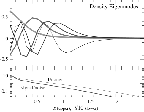
Figure 3: Principle components of the dark energy density $d\equiv\ln(\rho_{{\rm DE}}/\rho_{{\rm cr}0})$: (upper) first five eigenfunctions of the growth function (thick to thin) plotted in redshift; (lower) rank ordered inverse rms noise $\lambda_{\scriptscriptstyle i}^{\scriptscriptstyle-1/2}$ (thin) and signal-to-noise ratio in the fiducial model. Higher eigenfunctions pick up evolution in the dark energy density which is absent in the fiducial model.

Again, the recovery of finely-binned parameters is noisy and correlated across neighboring bins. The information content is best revealed through the Fisher principle component analysis. Shown in Fig. 3 (top) are the first 5 eigenfunctions. The qualitative difference between the eigenfunctions of the growth and that of the density is the presence of substantial low redshift information in the latter. The dark energy density at low redshift affects the distance to all higher redshifts. In Fig. 3 we show the eigenvalues as $\lambda_{\scriptscriptstyle i}^{\scriptscriptstyle-1/2}$ and the signal-to-noise ratio for the fiducial model and $f_{\rm sky}=0.1$.

It is again desirable to find an uncorrelated but more localized representation of the data. Unfortunately, the Fisher square-root technique of Eqn. (14) does not yield localized windows for the dark energy density. Instead we choose a close analogue, the Cholesky decorrelation HamTeg00 where the windows are the columns of ${\bf L}$ and ${\bf F}_{dd}={\bf L}{\bf L}^{t}$ again normalized to sum to unity. The windows are shown in Fig. 4 (lower panel). The windows also have the interesting property that they are strictly zero below some minimum redshift.

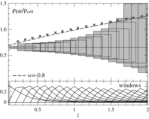
Figure 4: Localized constraints on the dark energy density: (upper) projected error boxes on the growth function with $1\sigma$ error bars around the fiducial model (line) for the Cholesky representation where band widths are taken from the window functions (lower). For comparison a model with $w=-0.8$ is shown both in the predictions for the modes (points) and the density function itself (curve). The small difference reflects the non-locality of the windows. Any deviation from constancy represents dark energy that is not a cosmological constant.

In Fig. 4 (upper panel) we show the projected constraints on these localized modes compared with the predictions for a $w=-0.8$ model (points) and the actual function $\rho_{{\rm DE}}(z)$ (curve) in this model. The deviation between the points and the curve reflects the non-locality of the windows. Note that for a cosmological constant model ($\rho_{{\rm DE}}=$ const.) there is no deviation by definition (straight line) and that the expectation value of all points is $\ln\Omega_{\rm DE}$. Any statistically significant difference in the values of the points in this reconstruction represent a detection of a dark energy component that is not a cosmological constant WanGar01 . This is true in spite of the non-locality of the windows and independently of the model-dependent parameterization of the dark energy.

Again one may always test specific models for the dark energy from the model-independent parameterization. Many dark energy models can be parameterized by $\Omega_{{\rm DE}}$, $w(z_{\rm eff})$, and $w^{\prime}=dw/dz|_{z_{\rm eff}}$. The pivot point $z_{\rm eff}$ can be chosen to be the best constrained redshift or “sweet spot” by decorrelating the errors in $w$ and $w^{\prime}$. As was the case for the growth rate, the resulting errors on $w(z_{\rm eff})$ are the same as in the case of a two parameter model $(\Omega_{{\rm DE}},w)$. For the fiducial model and survey, this is $z_{\rm eff}=0.33$ and $\sigma(w)=0.016f_{\rm sky}^{-1/2}$. Note that this constraint is marginalized over $(\Omega_{{\rm DE}},w^{\prime})$ without prior assumptions to their values.

As in the case of supernovae luminosity distance measures WelAlb02 ; MaoBruMcMSte02 , there remains a degeneracy between $\Omega_{{\rm DE}}$ and $w^{\prime}$ in that they may both be adjusted upward to keep the dark energy density at the well-constrained low redshifts fixed. In Fig. 5 shows, we show the $68\%$ confidence region with various assumptions of prior knowledge on $\Omega_{{\rm DE}}$: none, $\sigma(\Omega_{{\rm DE}})=0.03$, $=0.01$. With $\Omega_{{\rm DE}}$ fixed, the errors become $\sigma(w^{\prime})=0.046f_{\rm sky}^{-1/2}$. With no prior, the errors degrade to $\sigma(w^{\prime})=0.069f_{\rm sky}^{-1/2}$.

Conversely if $w^{\prime}$ is fixed, the constraints on the dark energy density improve to $\sigma(\Omega_{{\rm DE}})=0.003f_{\rm sky}^{-1/2}$. This two parameter family ($\Omega_{{\rm DE}},w$) represents the amplitude and slope of the dark energy density itself at a normalization point of $z=0$. The remaining degeneracy with $w$ can be removed by again going to the “sweet spot”, here $z=0.13$ where the errors on the dark energy density improve by a factor of 1.5. Again this also represents the errors on $\Omega_{{\rm DE}}$ in the single parameter family of dark energy models $\sigma(\Omega_{{\rm DE}})=0.002f_{\rm sky}^{-1/2}$. Errors on $w$ of course remain unchanged.

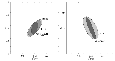
Figure 5: Error ellipses (68% CL) for dark energy parameters ($\Omega_{{\rm DE}}$, $w$, $w^{\prime}$): (upper) the ($\Omega_{{\rm DE}},w^{\prime}$) plane showing the degeneracy direction and the efficacy of external information on $\Omega_{{\rm DE}}$; (lower) the ($\Omega_{{\rm DE}},w$) plane with complete and no external information on $w^{\prime}$. Here $w$ is defined as the equation of state at $z=0.33$. The fiducial model and survey are assumed throughout with $f_{\rm sky}=0.1$.

V Discussion

We have shown that lensing surveys covering more than a few percent of the sky with good photometric redshift information can probe the time evolution of the linear growth function and distance-redshift relation, both of which are sensitive to properties of the dark energy and dark matter. Specifically, we have tested a model-independent parameterization of the linear growth rate and/or dark energy density discretized into bins in redshift. Deviations in the growth rate would indicate a component of the dark matter that is not effectively cold or dark energy that is not smooth on the lensing scale. Deviations in the constancy of the dark energy density would rule out a cosmological constant model.

In this exploratory study, we have made several simplifying assumptions that would need to be addressed in a concrete implementation. Perhaps the primary one is that future CMB measurements will completely fix the high redshift cosmology. The most uncertain piece involves the amplitude of the initial fluctuations on the scales relevant to the lensing pixels, $k\sim 0.05$ Mpc^-1 for degree scales. Fortunately, the pivot point of CMB anisotropy experiments with several arcminute scale resolution is sufficiently close to the lensing scale that the slope and shape of the initial power spectrum do not cause much ambiguity Hu01c .

To fully utilize the lensing information, the initial amplitude must be fixed to an accuracy better than the amplitude of the growth function, which we have found to be $\sim 0.002f_{\scriptscriptstyle\mathrm{sky}}^{\scriptscriptstyle-1/2}$, i.e. percent level accuracy for surveys of several thousand square degrees. For CMB anisotropies, this precision requires that the optical depth during reionization must be determined to $\sigma(\tau)\sim 0.01$ to resolve the amplitude degeneracy. If determined from CMB observations alone, this will require polarization measurements with a precision comparable to the Planck satellite planck , which can in principle achieve $\sigma(\ln\delta_{\zeta})=0.0044$ at $k=0.05$ Mpc^-1 Hu01c . Direct measurements of the reionization epoch can also resolve the ambiguity Hu01c . Even in the absence of this information, the evolution of the growth and luminosity-distance relation are still constrained. These issues are best addressed through joint parameter estimation.

On the lensing side, the most important assumption is that the noise in the convergence measurements is well-calibrated and not significantly larger than the projections based on intrinsic ellipticities. Even aside from the demanding requirements for control of systematic errors, there may be intrinsic correlations in the ellipticities intrinsic that need to be modeled or avoided by increasing the pixel scale and redshift bin widths. The recovered information is largely insensitive to the redshift bin width since the high signal-to-noise modes are all low frequency. Errors scale roughly as $A_{\rm pix}^{1/2}$ due to the loss of independent modes in a fixed survey area.

We have also neglected sample covariance between the pixels but note that we have correspondingly neglected the information contained in such correlations. Indeed, we have completely neglected the information contained in the non-linear regime which in fact contains the majority of the information from lensing tomography HuKee02 . Clearly, future studies will be required to see how best to mine the model-independent information contained in lensing tomography.

Acknowledgments: I thank D. Huterer and C.R. Keeton for useful conversations and E. Linder for pointing out a typo in the draft. This version includes errata from a coding bug, affecting constraints involving the present dark energy density, pointed out by K. Abazajian and S. Dodelson. WH is supported by NASA NAG5-10840 and the DOE OJI program.

References

- (1)
- (2) J.A. Tyson, R.A. Wenk, F. Valdes, Astrophys. J, 349, 1 (1990).
- (3) M. Bartelmann, P. Schneider, Phys. Rept., 340, 291 (2001); Y. Mellier, Ann. Rev. Astron. Astrophys., 37, 127 (1999); H. Hoekstra, H. Yee, M. Gladders, New Astron., in press, astro-ph/0205205 (2002).
- (4) D. Huterer, M.S. Turner, Phys. Rev. D, 64, 123527 (2001); L. Wang, R.R. Caldwell, J.P. Ostriker, P.J. Steinhardt, Astrophys. J, 530, 17 (2000).
- (5) R.D. Blandford, A.B. Saust, T.G. Brainerd, J.V. Villumsen, Mon. Not. Roy. Astr. Soc., 251, 600 (1991); J. Miralda-Escude, Astrophys. J, 380, 1 (1991); N. Kaiser, Astrophys. J, 388, 272 (1992).
- (6) D. Bacon, A. Refregier, R. Ellis, Mon. Not. Roy. Astr. Soc., 318, 625 (2000); N. Kaiser, G. Wilson, G.A. Luppino, Astrophys. J Lett., submitted, astro-ph/0003338 (2000); L. van Waerbeke, et al. Astron. Astrophys., 358, 30 (2000); D.M. Wittman, J.A. Tyson, D. Kirkman, I. Dell’Antonio, G. Bernstein, Nature, 405, 143 (2000).
- (7) D. Huterer, Phys. Rev. D, 65, 063001 (2002).
- (8) W. Hu, Phys. Rev. D, 65, 023003 (2002).
- (9) R.R. Caldwell, R. Dave, P.J. Steinhardt, Phys. Rev. Lett., 80, 1582 (1998).
- (10) W. Hu, Astrophys. J, 506, 485 (1998).
- (11) Y. Wang, P.M. Garnavich, Astrophys. J, 552, 445 (2001).
- (12) I. Maor, R. Brustein, J. McMahon, P.J. Steinhardt, Phys. Rev. D, 65, 123003 (2002).
- (13) J. Weller, A. Albrecht, Phys. Rev. D, 65, 103512 (2002).
- (14) M. Tegmark, Phys. Rev. D, submitted, astro-ph/0101345 (2001).
- (15) D. Huterer, G. Starkman, Phys. Rev. Lett., submitted, astro-ph/0207517 (2002).
- (16) D. Wittman, J.A. Tyson, V.E. Margoniner, J.G. Cohen, I.P. Dell’Antonio, Astrophys. J, 557, 89 (2001).
- (17) W. Hu, Astrophys. J Lett., 522, 21 (1999).
- (18) A.N. Taylor, Phys. Rev. Lett., submitted, astro-ph/0111605 (2001).
- (19) W. Hu, C.R. Keeton, Phys. Rev. D, in press, astro-ph/0205412 (2002).
- (20) M. Tegmark, A.N. Taylor, A.F. Heavens, Astrophys. J, 480, 22 (1997).
- (21) B. Jain, U. Seljak, Astrophys. J, 484, 560 (1997).
- (22) N. Kaiser, Astrophys. J, 498, 26 (1998).
- (23) A.J.S. Hamilton, M. Tegmark, Mon. Not. Roy. Astr. Soc., 312, 285 (2000).
- (24) J.F. Beacom, N.F. Bell, Phys. Rev. D, 65, 113009 (2002).
- (25) W. Hu, D.J. Eisenstein, M. Tegmark, Phys. Rev. Lett., 80, 5255 (1998).
- (26) O. Elgaroy, et al. Phys. Rev. Lett., in press, astro-ph/0204152 (2002).
- (27) D.J. Eisenstein, W. Hu, M. Tegmark, Astrophys. J, 518, 2 (1999).
- (28) http://astro.estec.esa.nl/Planck
- (29) P. Catelan, M. Kamionkowski, R.D. Blandford, Mon. Not. Roy. Astr. Soc., 323, 713 (2001); R. Crittenden, P. Natarajan, U. Pen, T. Theuns, Astrophys. J, 559, 552 (2001); R.A.C. Croft, C. Metzler, Astrophys. J, 545, 561 (2000); A.F. Heavens, A. Refregier, C. Heymans, Mon. Not. Roy. Astr. Soc., 319, 649 (2000).