The Neupert effect in solar flares and implications
for coronal heating

Abstract

Based on simultaneous observations of solar flares in hard and soft X-rays we studied several aspects of the Neupert effect. About half of 1114 analyzed events show a timing behavior consistent with the Neupert effect. For these events, a high correlation between the soft X-ray peak flux and the hard X-ray fluence is obtained, being indicative of electron-beam-driven evaporation. However, for about one fourth of the events there is strong evidence for an additional heating agent other than electron beams. We discuss the relevance of these findings with respect to Parker’s idea of coronal heating by nanoflares.

1 Introduction

The Neupert effect is the name given to the observational finding that the rising part of the soft X-ray (SXR) light curve often resembles the time integral of the hard X-ray (HXR) or microwave emission (Neupert, 1968; Dennis & Zarro, 1993). The physical relevance of the Neupert effect basically arises from the fact that it is interpreted as a causal connection between the thermal and nonthermal flare emissions, which can be naturally explained within the nonthermal thick-target model (Brown, 1971). In this model, the flare energy is released primarily in the form of nonthermal electrons, and hard X-rays are produced via electron-ion bremsstrahlung when the electron beams impinge on the lower corona, transition region and chromosphere. The model assumes that only a small fraction of the electron beam energy is lost through radiation; most of the loss is due to Coulomb collisions that serve to heat the ambient plasma. As a consequence of the rapid energy deposition a strong pressure imbalance develops between the dense, heated chromosphere and the tenuous corona. The high pressure gradients cause the heated plasma to convect into the corona in a process known as chromospheric evaporation (Antonucci et al. 1984; Fisher et al. 1985), where it gives rise to enhanced SXR emission via thermal bremsstrahlung.

In this case, the hard X-ray flux is linked to the instantaneous rate of energy supplied by electron beams, whereas the soft X-ray flux is related to the accumulated energy deposited by the same electrons up to that time, and we can expect to see the Neupert effect. Any deviation from the Neupert effect, in principle, suggests that the hot SXR emitting plasma is not heated exclusively by thermalization of the accelerated electrons that are responsible for the HXR emission. Therefore, investigations of the Neupert effect provide insight into the role of nonthermal electrons for the flare energetics.

The Neupert effect can be expressed as

$$F_{\rm P,SXR}=k\cdot{\cal F}_{\rm HXR},$$ (1)

with $F_{\rm P,SXR}$ the SXR peak flux and ${\cal F}_{\rm HXR}$ the HXR fluence, i.e. the HXR flux integrated over the event duration. The coefficient $k$ depends on several factors, as, e.g., the magnetic field geometry and the viewing angle, and thus may vary from flare to flare (Lee et al., 1995). However, if $k$ does not depend systematically on the flare intensity, then the SXR peak flux and the HXR fluence are linearly related.

2 Data Selection

We utilize the SXR data from the Geostationary Operational Environmental Satellites (GOES) and the HXR data from the Burst and Transient Source Experiment (BATSE) aboard the Compton Gamma Ray Observatory. The X-ray sensor aboard GOES consists of two ion chamber detectors, which provide whole-sun X-ray fluxes in the 0.5–4 and 1–8 Å wavelength bands. BATSE is a whole-sky HXR flux monitor that, in part, consists of eight large-area detectors. From each detector there are hard X-ray measurements in four energy channels, 25–50, 50–100, 100–300 and $>$300 keV (Schwartz et al., 1992).

For the analysis, the 1-min averaged GOES SXR data measured in the 1–8 Å channel and the HXR data collected in the BATSE Solar Flare Catalog, archived in the Solar Data Analysis Center at NASA/Goddard Space Flight Center for the period 01/1997 – 06/2000 are used. The peak and total count rates are background subtracted for the flux below 100 keV. For the SXR events, we used the flux just before the flare start for background subtraction. To be identified as corresponding events we demand that the start time difference between a SXR and a HXR event does not exceed 10 min. Overlapping events are excluded. Applying these criteria, we obtained 1114 events that were observed in both hard and soft X-rays (for details see Veronig et al., 2002a).

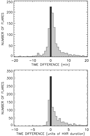
Figure 1: Histogram of the difference of the SXR maximum and the HXR end time in absolute values (top panel) and normalized to the HXR event duration (bottom panel). Positive values indicate that the maximum of the SXR emission occurs after the end of the HXR emission, negative values vice versa.

3 Analysis

For each event we determined the difference, $\Delta t$, of the peak time of the SXR emission, $t_{\rm SXR,P}$, and the end time of the HXR emission, $t_{\rm HXR,E}$. Furthermore, the time differences were normalized to the duration $D$ of the respective HXR event, i.e.

$$\Delta t_{\rm norm}=\frac{\Delta t}{D}=\frac{t_{\rm SXR,P}-t_{\rm HXR,E}}{D}\,.$$ (2)

Figure 1 shows the histogram of the absolute and normalized time differences. Both representations of the SXR–HXR time difference have its mode at zero. 49% of the events lie within the range $|\Delta t|\leq 1$ min, and 65% within $|\Delta t|\leq 2$ min. For the normalized time differences, we obtain that 44% lie within $|\Delta t_{\rm norm}|\leq 0.5$ HXR units, and 59% within $|\Delta t_{\rm norm}|\leq 1$ HXR unit. This outcome suggests that certainly a considerable part of the events coincides well with the expectations from the Neupert effect regarding the relative timing.

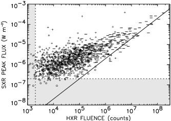
Figure 2: Scatter plot of the SXR peak flux versus the HXR fluence. The regions that lie beyond the estimated HXR fluence and SXR peak flux thresholds are grey shaded. Moreover, we have indicated the sign of the time difference between SXR peak and HXR end for each single event: “$+$” symbols denote events with positive, “$-$” symbols events with negative, “$\circ$” symbols events with zero time difference (i.e. the SXR peak and HXR end take place within $1$ min). The straight line indicates a line of constant $k$, i.e. $F_{\rm P,SXR}=2\cdot 10^{-12}\cdot{\cal F}_{\rm HXR}$.

Figure 2 shows the scatter plot of the SXR peak flux versus the HXR fluence for the complete sample, clearly revealing an increase of $F_{\rm P,SXR}$ with increasing ${\cal F}_{\rm HXR}$. It can also be inferred from the figure that the slope is not constant over the whole range but that it is larger for large HXR fluences than for small ones. For very large fluences, the slope approaches the value of 1, indicative of a linear relation between the SXR peak flux and HXR fluence. We stress that the slope at small fluences might be affected by missing events with small SXR peak fluxes (due to selection effects), and thus appear flatter than it is in fact. Figure 2 reveals an interdependence between the importance of an event and the sign of the time difference. Basically all large flares belong to the group of events with $\Delta t<0$, i.e. the SXR peak occurs before the HXR end. Moreover, the flares with $\Delta t<0$ reveal a strong tendency to be of long duration.

We obtain a high cross-correlation coefficient for the SXR peak flux and HXR fluence relationship, $r=0.71$. This coefficient is higher than those for the SXR peak flux and HXR peak flux, $r=0.57$. This indicates that the correlation is primarily due to the HXR fluence – SXR peak flux relationship, as predicted from the Neupert effect, and not, e.g., due to the fact that flares with large HXR peak fluxes also tend to have intense SXR counterparts. Furthermore, it is important to note that the HXR fluence – SXR peak flux correlation is higher for the events with negative time differences, $r=0.82$, than for the events with positive time differences, $r=0.54$.

On the basis of the relative timing of the SXR peak and the HXR end, we extracted two subsets of events. The events of set 1 are roughly consistent with the timing expectations of the Neupert effect, and the events of set 2 are inconsistent with it. The two sets are defined by the following conditions:

$${\rm Set~{}1:~{}}(|\Delta t|<1{\rm~{}min}) {\rm OR} (|\Delta t_{\rm norm}|<0.5{\rm~{}unit})\,,$$

$${\rm Set~{}2:~{}}(|\Delta t|>2{\rm~{}min}) {\rm AND} (|\Delta t_{\rm norm}|>1.0{\rm~{}unit})\,.$$

The applied conditions represent a combination of absolute and normalized time differences in order to avoid as much as possible any a priori interdependence with the flare duration and/or flare intensity. Out of the 1114 corresponding HXR and SXR flares, 485 (44%) events fulfilled the timing criterion of set 1; 270 events (24%) belong to set 2; 359 events (32%) are neither attributed to set 1 nor to set 2.

In Figure 3, we plot the SXR peak flux versus the HXR fluence separately for set 1 and set 2. The figure reveals that the two sets have very different characteristics besides the different timing behavior. Set 1 contains many more large events and shows a steeper increase of $F_{\rm P,SXR}$ with increasing ${\cal F}_{\rm HXR}$ than set 2. Moreover, set 1 contains more events with negative than positive time difference, whereas almost all events of set 2 are characterized by $\Delta t>0$, i.e. increasing SXR emission beyond the end of the hard X-rays. On average, for small fluences the events belonging to set 2 have a larger SXR peak flux at a given HXR fluence than those of set 1, indicating an “excess” of SXR emission with respect to set 1. The cross-correlation coefficients derived separately for the subsets reveal that the correlation among the SXR peak flux and HXR fluence is much more pronounced for the events of set 1, $r=0.78$, than those of set 2, $r=0.41$.

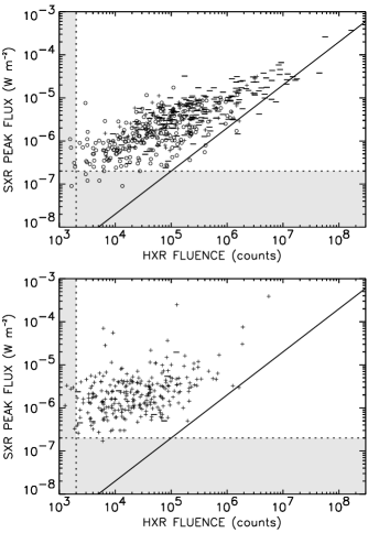
Figure 3: Scatter plot of the SXR peak flux versus the HXR fluence separately plotted for set 1 (top panel) and set 2 (bottom panel). The straight lines are lines of constant $k$ $(=2\cdot 10^{-12})$.

Figure 4: Flare frequency distributions as function of the SXR peak flux (top panel) and HXR fluence (bottom panel). The straight line indicates the linear fit in log-log space, characterized by a slope $-\alpha$.

4 Discussion and Conclusions

24% of the events have $\Delta t<0$, i.e. the SXR maximum occurs before the end of the HXR emission. These events are preferentially of long duration. Li et al. (1993) have calculated time profiles of soft and hard X-ray emission from a thick-target electron-heated model, finding that, in general, the time derivative of the SXR emission corresponds to the time profile of the HXR emission, as stated by the Neupert effect. However, for gradual events they obtained that this relationship breaks down during the decay phase of the HXR event, in that the maximum of the SXR emission occurs before the end of the HXR emission. This phenomenon can be explained by the fact that the SXR emission starts to decrease if the evaporation-driven energy supply cannot overcome the instantaneous cooling of the hot plasma, which is likely to happen in gradual flares. Considering our observational findings together with the results from simulations by Li et al. (1993), presumably most of the events with $\Delta t<0$ are consistent with the electron-beam-driven evaporation model. In particular, the high correlation between $F_{\rm P,SXR}$ and ${\cal F}_{\rm HXR}$, $r\approx 0.8$, supports such interpretation.

56% of the events have $\Delta t>0$; these events are preferentially of short and weak HXR emission. In principle, the fact that the SXR emission is still increasing although the HXR emission, i.e. the electron input, has already stopped indicates that an additional agent besides the HXR emitting electrons is contributing to the energy input and prolonging the heating and/or evaporation. However, McTiernan et al. (1999) have shown that the SXR time profile depends on the temperature response of the used detector: An increase of the SXR emission of low-temperature flare plasma after the HXR end may arise due to cooling of high-temperature plasma. Thus, we cannot attribute all events with $\Delta t>0$ as inconsistent with the electron-beam-driven chromospheric evaporation model. Instead, we consider as inconsistent only flares which show strong deviations from $\Delta t=0$, i.e. the events belonging to set 2.

This means that for at least one fourth of the analyzed events an additional heating agent besides nonthermal electrons is suggested. A probable scenario is that energy is transported from the primary energy release site via thermal conduction fronts, which initiate chromospheric evaporation but do not produce hard X-rays. The finding that for a considerable fraction of flares, preferentially weak ones, an additional heating agent other than electron beams is suggested, is not only relevant for the flare energetics but also for Parker’s idea of coronal heating by nanoflares (Parker, 1988).

Hudson (1991) pointed out that if the corona is heated by flare-like events of different sizes, then the flare energy distribution must have a power-law slope $\alpha>2$. If the SXR flux does not vary systematically with temperature and density, then the SXR peak flux is linearly related to the maximum thermal energy of the flare plasma (see Lee et al., 1995; Veronig et al., 2002a). On the other hand, HXR fluence distributions can be considered as representative for the energy contained in nonthermal electrons. In Figure 4, we show the SXR peak flux and the HXR fluence distributions derived from 1114 corresponding SXR/HXR flares, finding $\alpha=1.95$ $\pm$ 0.13 and $\alpha=1.58$ $\pm$ 0.13, respectively. The discrepancy between the slopes of the HXR fluence and the SXR peak flux distributions was already pointed out and discussed in Lee et al. (1993, 1995) and Veronig et al. (2002b). The present analysis provides an explanation for this difference in power-law slopes: The relationship between the SXR peak flux and the HXR fluence is not linear, whereby the deviations from a linear correlation are strongest for weak flares (cf. Figure 2).

The soft X-ray flare emission increases due to energy supply by electron beams as well as any other heating agent, whereas the hard X-ray emission contains only information on the energy provided by electrons. Together with our finding that particularly in weak events an additional heating agent besides electron beams is suggested, this strongly suggests that soft X-ray peak flux distributions are a more meaningful indicator of flare energy distributions than hard X-ray fluence distributions. Furthermore, we have shown that weak flares have different characteristics than large flares, in the sense that electrons are less important for their energetics. Therefore, it is possible that the power-law slope of nanoflare frequency distributions differs from that derived for observed flares, which is close to the critical value of $2$. In this respect it should be worthwhile to investigate flare frequency distributions of SXR flares without HXR counterparts, i.e. without detectable particle acceleration, since these flares possibly provide the link to the smallest flare-like energy release events.

References

- [1] Antonucci E., Gabriel A. H., Dennis B. R., 1984, ApJ 287, 917
- [2] Brown J. C., 1971, Solar Phys. 18, 489
- [3] Dennis B. R., Zarro D. M., 1993, Solar Phys. 146, 177
- [4] Fisher G. H., Canfield R. C., McClymont A. N., 1985, ApJ 289, 425
- [5] Hudson H. S., 1991, Solar Phys. 133, 357
- [6] Lee T. T., Petrosian V., McTiernan J. M., 1993, ApJ 412, 401
- [7] Lee T. T., Petrosian V., McTiernan J. M., 1995, ApJ 448, 915
- [8] Li P., Emslie A. G., Mariska J. T., 1993, ApJ 417, 313
- [9] McTiernan J. M., Fisher G. H., Li P., 1999, ApJ 514, 472
- [10] Neupert W. M., 1968, ApJ 153, L59
- [11] Parker E. N., 1988, ApJ 330, 474
- [12] Schwartz R. A., Dennis B. R., Fishman G. J., et al., 1992, NASA CP-3137, 457
- [13] Veronig A., Vršnak B., Dennis B. R., Temmer M., Hanslmeier A., Magdalenić J., 2002a, A&A revised
- [14] Veronig A., Temmer M., Hanslmeier A., Otruba W., Messerotti M., 2002b, A&A 382, 1070