ON THE ABUNDANCE OF HOLMIUM IN THE SUN

Abstract

The abundance of holmium (Z = 67) in the Sun remains uncertain. The photospheric abundance, based on lines of Ho II, has been reported as $+0.26\pm 0.16$ (on the usual scale where log(H) = 12.00), while the meteoretic value is $+0.51\pm 0.02$. Cowan code calculations have been undertaken to improve the partition function for this ion by including important contributions from unobserved levels arising from the (4f¹¹6p + 4f¹⁰(5d + 6s)²) group. Based on 6994 computed energy levels, the partition function for Ho II is 67.41 for a temperature of 6000 K. This is $\approx$1.5 times larger than the value derived from the 49 published levels. The new partition function alone leads to an increase in the solar abundance of Ho to log(Ho) $=+0.43$. This is within 0.08 dex of the meteoretic abundance. Support for this result has been obtained through LTE spectrum synthesis calculations of a previously unidentified weak line at $\lambda_{\odot}3416.38$. Attributing the feature to Ho II, the observations may be fitted with log(Ho) = +0.53. This calculation assumes log$(gf)=0.25$ and is uncertain by at least 0.1 dex.

guessConjecture

1 Introduction

The abundances of most nonvolatile elements in CI chondrites are in close agreement with those determined for the solar photosphere (Grevesse and Sauval, 1998; hereafter GS). The lanthanide holmium is one of only a few elements with differences of the order of 0.3 dex or more. GS give log(Ho_CI)$-$log(Ho_⊙) $=+0.25$.

The solar abundance of holmium reported by GS is $+0.26\pm 0.16$ and is based on an unpublished analysis of Ho II, the dominant ion in the Sun, by Daems, Biémont, and Grevesse (hereafter DBG) in 1984. Four lines at $\lambda$3343.6, 3398.9, 3456.0, and 3474.2 Å were analyzed. All of the features are blended, with the holmium lines constituting only minor contributors to the observed spectrum (N. Grevesse, private communication). The scatter about the mean abundance in this study arises partly from problems of blending and partly from the uncertainty in the adopted $gf$-values from Gorshkov and Komarovskii (1979). The partition function for Ho II was calculated using the known atomic levels at the time; at 6000 K, the value was found to be 43.8 (N. Grevesse, private communciation).

The published level structure for Ho II is seriously incomplete (cf. Martin, Zalubas, and Hagan, 1978; hereafter MZH): only 49 levels are known, many with no term designations and a few with multiple J-values. Wyart, Koot, and van Kleef (1974) note that a satisfactory analysis of this ion requires the calculation of the (4f¹¹6p + 4f¹⁰(5d + 6s)²) group. Of particular importance are the contributions from the 4f¹⁰6s² and 4f¹⁰5d6s configurations which are expected to begin below 12 000 cm^-1 (Brewer, 1971). Only eight measured levels have energies lying below this threshold.

Much of the difference between the meteoritic abundance of holmium and that found by DBG in the Sun may be due to an underestimate of the partition function for Ho II. Cowan-code calculations were therefore undertaken to supplement the published data. In addition, a fresh examination of the solar spectrum was made in an attempt to identify additional, weak, unblended features that might be attributable to Ho II and used in spectrum synthesis calculations to establish an independent estimate of the abundance of this element. One line in particular, at 3416.38 Å, was found to be amenable to such analysis.

In the following section, we describe the energy level calculations and give the partition functions that result from them for temperatures in the range 3000 to 34 000 K. The third section addresses our search for other Ho II lines suitable for analysis by spectrum synthesis techniques, while in the fourth, the results of our study of the $\lambda$3416 line are presented. The final section of the paper briefly summarizes the current state of our knowledge of the abundances of the lanthanide rare-earth elements in the Sun vis-a-vis the CI chondrites; it also includes some remarks about our recent re-examination of the abundance of the volatile element indium in the Sun.

2 Energy Level Calculations and Partition Functions

The methodology employed in making the energy level calculations is based on the Cowan code (Cowan, 1981; 1995) and follows that described by Bord (2000, and references cited therein). Briefly, single-particle radial wavefunctions were determined using a Hartree plus statistical exchange interaction approximation for the following even and odd parity configurations, respectively: (4f¹¹6p + 4f¹⁰(5d + 6s)²) and ($4f^{11}6s+4f^{11}5d$). Experimental energy levels exist for three of these configurations, viz. 4f¹¹6p, $4f^{11}6s$, and $4f^{11}5d$, but none is complete. Relativistic and electron correlation corrections have been included in the calculations, and the eigenvectors were constructed using both LS- and jj-coupling basis sets. J₁j-coupling is best suited to describe the electron interactions in this ion.

Ab initio values for the single-configuration center-of-gravity energies and the various radial and configuration interaction integrals were computed with uniform scaling applied to all spin-orbit and Slater parameters. Reducing the theoretical values of F${}^{\emph{k}}$ and G${}^{\emph{k}}$ in this manner roughly accounts for the effects of introducing additional two-body electrostatic operators for legal values of k. The adopted scale factor for the Slater parameters was 0.68, while that for the spin-orbit interaction was 0.96. These values are typical of what has been used in our previous studies of lanthanide rare-earth ions and comport well with values published by other workers applying the Cowan code in the analysis of these species (cf. Zhang, et al., 2002, and references cited therein).

The radial integrals for the odd levels were optimized to fit the known energy levels using the method of least squares. A total of 468 levels were computed, of which 19 (all that are known) were fitted, including the ground state. In as much as the number of known levels equalled the number of structure parameters to be determined, several of the latter had to be held fixed and/or linked together in order to secure convergence of the least squares procedure. After considerable experimentation with various combinations, the final fit with 9 free parameters yielded a mean deviation in energy of 156 cm^-1 or $\approx$0.8% over a range of 20 000 cm^-1.

Among the even configurations, 6526 levels were calculated. Since only 11 levels possessing reliable energies have been completely classified, all belonging to the 4f¹¹6p configuration (which requires 9 parameters alone for its description), no attempt was made to refine the structure parameters by fitting the measured energies. Instead, the center-of-gravity energies for each configuration were shifted to produce agreement between the calculations and the known (in the case of 4f¹¹6p) or predicted (for 4f¹⁰5d², 4f¹⁰5d6s, and 4f¹⁰6s²) energies for the lowest lying levels in each. In the latter configurations, the estimates of Brewer (1971) were used.

Comparisons between the post-shifted calculations and the measured energies in the 4f¹¹6p configuration revealed differences of $\leq 500$ cm^-1 over a range of 30 000 cm^-1 (or $\approx$2%). This is typical, in our experience, of the agreement between the raw (i.e., un-fitted) calculations and the experimental energies in rare-earth ions and suggests that similar “agreement” may be expected for the low-lying levels in the unobserved (4f¹⁰(5d + 6s)²) group. Adopting 500 cm^-1 as the uncertainty yields an estimated acuracy of $\approx$5% for the 4f¹⁰6s² and 4f¹⁰5d6s configurations that begin at about 10 000 cm^-1 and 11 500 cm^-1, respectively.

Partition functions for the range 3000 K to 34 000 K were calculated based on the 6994 Cowan-code levels following the methodology of Radziemski and Mack (1980) and Cowley and Barisciano (1994). Where an unambiguous assignment based on the MZH compilation could be made, the measured energies were substituted for the calculated values. Table I shows the results of our computations compared to those that would be found using only the known/published energies. As may be seen, at 6000 K, the new partition function is more than 50% larger than that found from the levels tabulated in MZH and used by DBG. This difference is primarily due to a nearly 12-fold increase in the number of energy levels in the range 10 000 to 30 000 cm^-1 over what appears in MZH. As Grevesse (1984) has pointed out, these levels are especially important for determining the partition functions for ions in the Sun.

Table 1: Partition functions for Ho II

Temp	This	NIST	Temp	This	NIST
(K)	Work	Levels	(K)	Work	Levels
3000	31.09	30.31	19 000	1651.95	154.08
4000	37.90	34.09	20 000	1902.26	163.40
5000	49.39	38.51	21 000	2169.26	172.59
6000	67.41	43.63	22 000	2451.98	181.64
7000	93.93	49.50	23 000	2749.42	190.52
8000	131.02	56.09	24 000	3060.54	199.23
9000	180.77	63.35	25 000	3384.30	207.75
10 000	245.11	71.21	26 000	3719.68	216.09
11 000	325.76	79.57	27 000	4065.66	224.24
12 000	424.08	88.34	28 000	4421.26	232.19
13 000	541.11	97.41	29 000	4785.55	239.95
14 000	677.53	106.70	30 000	5157.61	247.51
15 000	833.65	116.13	31 000	5536.60	254.89
16 000	1009.51	125.64	32 000	5921.68	262.07
17 000	1204.86	135.16	33 000	6312.10	269.08
18 000	1419.22	144.66	34 000	6707.13	275.90

To estimate the sensitivity of the partition functions to uncertainties in the new, calculated energies, all of which have values greater than 10 000 cm^-1, several numerical tests were performed. In one series of experiments, the energies were randomly incremented and decremented first by 500 cm^-1 and then 1000 cm^-1 and the partition functions recalculated using the shifted energy values. At 6000 K, the change in the partition function was $\leq 1\%$ in each case. Systematically adding 500 cm^-1 to every calculated energy level produces a partition function 4.6% smaller at 6000 K than that given in Table I; subtracting the same amount from each calculated energy raises the partition function at this temperature by 5.2%. Thus, at temperatures relevant for studies of the Sun, we conclude that the expected uncertainties in the calculated energies lead to errors in the partition function of $\approx$5% or less. This source thus contributes an uncertainty of $\leq 0.02$ dex to the abundance determination of holmium in the Sun (see below).

The results presented in Table I also comport favorably with the calculations done by Cowley (1984) based on approximations to the level structure using skewed Gaussians to correct for incompleteness. Although this approach is limited in its usefulness at relatively low temperatures like that of the Sun, a comparison between Cowley’s partition function for Ho II at 5000 K with that interpolated from Table I reveals the present Cowan-code–based value to be only $\approx$7% higher.

Table II gives the empirical fit to the interpolation formula for the partition function adopted by Bolton (1970), who used a polynomial in $\mathrm{ln}\,\theta$ (where $\theta=5040/T$):

$$\mathrm{ln}(u-g_{0})=\sum_{i=0}^{n}a_{i}(\mathrm{ln}\,\theta)^{i}.$$ (1)

Here $u$ is the partition function and $g_{0}$ is the statistical weight of the ground level. The fits to the energy sums with $n=4$ are within 1% or less for every temperature given in Table I. Investigators who prefer to use their own interpolation formulae may obtain the energy levels in machine-readable form from the first author at bord@astro.lsa.umich.edu.

Table 2: Parameters for polynomial fit to the partition function for Ho II

$g_{0}$	$a_{0}$	$a_{1}$	$a_{2}$	$a_{3}$	$a_{4}$
17.0	3.491604	-2.318539	1.084289	0.511300	0.036714

Insofar as the relative number of absorbers scales inversely with the partition function, the larger the partition function, the greater the required abundance of the species needed to match the observed line strength. At the temperature of the Sun (5770 K), increasing the partition function by a factor of 1.48 forces an increase in the holmium abundance of 0.17 dex. This yields a value of log(Ho) = +0.43, based on the earlier results (DBG). Even with no other changes, this brings the abundance of holmium within 0.08 dex of the meteoritic value. The estimated uncertainties in the computed energies and, hence, in the new partition function add negligibly to the errors quoted by DBG ($\pm 0.16$ dex).

3 Holmium Line Identifications

Moore, Minnaert, and Houtgast (1966; hereafter MMH) include no lines of Ho II in their count of individual spectra in the Sun. Grevesse and Blanquet (1969) searched for the strongest Ho II lines in the solar spectrum and found that all but seven were masked by well-identified lines, including three of those ultimately used by DBG. Because of differences between the laboratory wavelengths of the seven surviving lines and those of unidentified solar lines ranging from 0.013 to 0.083 Å, these authors concluded that it was premature to associate any solar feature entirely with Ho II.

Only four of the seven Grevesse-Blanquet (GB) candidate lines have been classified and have published $gf$-values. We have carefully re-examined the solar spectrum in the vicinity of where these lines might be found. Our purpose was to see if a compelling case could be made for an identification that could potentially produce an accurate holmium abundance by spectrum synthesis. Our survey revealed no good candidates from among the four lines considered. We briefly note the results of our investigations below:

$\mathbf{\lambda 4045.4}$: This line was suggested by GB for association with a 9 mÅ feature reported by MMH at $\lambda_{\odot}4045.508$. No local minimum was discernible near this wavelength in high resolution solar spectra obtained at Kitt Peak (Neckel, 1999) or the Jungfraujoch station (Delbouille and Roland, 1995). The putative feature is likely hidden in the wing of the very strong Fe I line at $\lambda_{\odot}4045.825$. This Ho line has been used, however, in the determination of the holmium abundance in the metal-poor halo giant $\rm{CS}\,22892-052$ by Sneden, et al. (1996).

$\mathbf{\lambda 3796.7}$: This line, arising from the ground level and having log($gf$) $=0.20$, has also been used in the analysis of $\rm{CS}\,22892-052$. In the Sun, an unidentified 33 mÅ feature at $\lambda_{\odot}3796.803$ appears much too strong to represent a reliable candidate for a holmium identification.

$\mathbf{\lambda 3474.2}$: This line was suggested by GB for identification with a 5.5 mÅ feature at $\lambda_{\odot}3474.273$, and was included in the analyses of DBG. This feature is a blend of two Fe I lines ($\lambda\lambda 3474.26$ and 3474.27), a line of Dy II ($\lambda 3474.27$), and the holmium line, with the latter being a distinctly minority contributor to the feature. Indeed, we were able to satisfactorily fit the observed solar feature by spectrum synthesis by including only the dysprosium and iron lines at their solar abundances. Adding the holmium line at the CI abundance produced no discernible change in the calculated profile; this occurs in large part because the hfs of this feature shifts the strongest component of the red-degraded flag pattern to 3474.160 Å in the wing of a very strong Mn II line. Although our results are thus compatible with a holmium abundance equal to that found in the meteorites, the insensitivity of this feature to variations in the holmium abundance makes it unsuitable for a definitive test of the amount of this element in the Sun.

$\mathbf{\lambda 3416.4}$: This line will be discussed in the next section.

A fifth Ho II line at $\lambda 4152.59$, not included by GB, was also considered by us as a candidate for analysis. This line has also been used by Sneden, et al. (1996) in their analysis of $\rm{CS}\,22892-052$, and was posited by us for association with an unidentified 8 mÅ line at $\lambda_{\odot}4152.527$ in the Sun (MMH). We computed the hfs splitting of the levels involved in the transition producing this line, taking the A and B parameters for the lower level from Worm, Shi, and Poulsen (1990) and those for the upper level from Sneden, et al. (1996). The computed energy shifts (in cm^-1) were applied to the “mean position” (also in cm^-1) of the line to produce the hfs pattern. The appropriate “mean position” to use was not obvious, however. Monograph 145 (Meggers, Corliss, and Scribner, 1975) gives $\lambda_{lab}=4152.61$ Å; Sugar (1968) reports a wavelength of 4152.62 Å, and, based on the energy levels in MZH, we compute a wavelength of 4152.59 Å. Sneden, et al. (1996) adopted 4152.58 Å in their study. Nave (2001, private communication) has recently measured this feature on a high resolution FTS spectrum and gives the center-of-gravity wavelength as 4152.604 Å. Using this value, we find the strongest hf component to lie at 4152.441 Å, in excellent agreement with Nave’s hfs measurements. These calculations place the bulk of the holmium absorption near 4152.45 Å at a local maximum in the solar spectrum and far from the observed $\lambda_{\odot}4152.53$ feature. In light of this discordance, further exploration of this line was abandoned in favor of the more promising feature near 3416.4 Å.

4 Spectrum Synthesis of the $\lambda 3416.4$ Feature

The $\lambda 3416$ line in Ho II arises from the following transition: $637.40(J=7)-29899.21(J=7)$. Precision FTS data put the center-of-gravity wavelength at 3416.444 Å (G. Nave, private communication). The hfs constants A and B for both the upper and lower levels of this transition are given by Worm, Shi, and Poulsen (1990) and yield a wavelength of 3416.376 Å for the strongest component of the primary octet pattern. This value compares very favorably with the position of a feature at 3416.375 Å in the Jungfraujoch solar spectrum for which we measure an equivalent width of 6.4 mÅ. MMH report a feature with $\lambda_{\odot}=3416.409$ Å and $W_{\lambda}=6$ mÅ, but give no identification. We adopt log($gf$)$=0.25\pm 0.04$ based on Nave’s transition probability; this is in good agreement with the VALD value of 0.23 for this transition (Kupka, et. al., 1999).

A 2.25 Å segment centered on $\lambda 3416.4$ was synthesized in LTE using the suite of programs described by Cowley (1996) and compared to both the Jungfraujoch and Kitt Peak solar spectra. The observed spectra are practically indistinguishable in the vicinity of the $\lambda 3416$ feature, and both yield a relative minimum in the continuum at $3416.375\pm 0.001$ Å.

Line data for atomic species (excepting holmium) were extracted from VALD, and the molecular data were taken from Kurucz (1993). Observed and predicted features for the (0,0), (1,1), and (2,2) bands of NH were included in the calculations, although only the transitions with the lowest J-values for the (2,2) system were used; the higher series members are weak and/or absent due to pre-dissociation at the temperature of the Sun. Small modifications to the Kurucz wavelengths for NH, typically amounting to less than $0.005$ Å, were made based on the energy levels published by Brazier, Ram, and Bernath (1986). Solar abundances (GS) of all atomic species save holmium were adopted, and the NH abundance was reduced by a factor of 0.55 from its equilibrium value derived using the solar abundances of N and H in order to achieve acceptable fits to the observed lines.

A 137-step model atmosphere based on the $T(\tau)$ given by Holweger and Müller (1974) was employed in this study. A 137-step version of a Kurucz model atmosphere with $l/h=0.75$ and no convective overshoot (R. Kurucz, private comunication) was also tested for comparison. It predicted a slightly higher continuum level in the vicinity of the $\lambda 3416$ feature, which led to the need to reduce the optimum holmium abundance (see below) by 0.1 dex in order to reconcile the calculations to the observations. This suggests that uncertainties in the model atmosphere and the adopted atomic parameters produce errors in the final solar holmium abundance of between 0.10 and 0.15 dex overall.

The spectrum was calculated in units of the specific intensity in double precision with the following model parameters: $vsini=0.0$ km s^-1 and $v_{turb}=1.0$ km s^-1. The computed spectrum was broadened using a Gaussian with half width 0.018 Å to match the resolution of the observations. The continuous opacity was also increased by a factor of 1.2 to achieve agreement between the calculated emergent intensity and the measurements of Neckel and Labs (1984) at 3400 Å.

Figure 1 compares the spectrum synthesis (solid line) with the observations (dotted line) assuming no holmium is present in the Sun. The absence of holmium in the model calculations makes it impossible to fit the observations near 3416.4 Å despite the generally good agreement between the synthesized spectrum and the solar data throughout most of the remainder of the region. (A notable exception is the unidentified feature at $\lambda_{\odot}3416.51$ discussed below.) Clearly, some opacity due to this element is required in order to reconcile the calculations with the observations. The issue remains, how much holmium is needed.

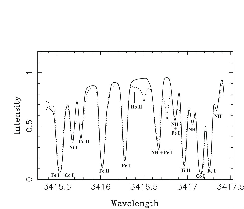
Figure 1: Synthesis (solid line) of the $\lambda 3416.4$ region of the solar spectrum with no absorption due to holmium included in the model. The observed Jungfraujoch spectrum is indicated with the dotted line and is not fit at all by the computations in the vicinity of the putative Ho II feature at 3416.38 Å. Remaining identifications are from MMH; absorptions of unknown origin are indicated by question marks. No attempt has been made to improve the overall fit by including the hfs of the cobalt lines, although some adjustments to the wavelengths and $gf$-values of a few lines were made to achieve better agreement with the observations as described in the text.

It should be noted that in Figure 1, no attempt has been made to improve the fit by including the hfs of the cobalt lines appearing in the region, although some adjustments to the VALD $gf$-values of a few lines (e.g. Ni I $\lambda 3415.68$ and Fe II $\lambda 3416.09$) were made to achieve better agreement with the observations. Also, because of its potential influence on the structure of the spectrum immediately to the blue of the Ho II feature at 3416.38 Å, care was taken to fit the Fe I line at 3416.28 Å as well as possible. In particular, small adjustments have been made in the VALD-values of the log($gf$) (reduced by 0.2 dex), the wavelength (reduced by 0.003 Å), and the damping width (increased by 20%). As it turned out, when tests were made, it was discovered that the best-fit holmium abundance was insensitive at the level of less than 0.05 dex to the modest modifications of the VALD values proposed above. In the figures that follow, the calculations have incorporated the modified choices for these parameters.

MMH also identify a feature at $\lambda_{\odot}3416.512$ as a predicted line of Fe I, but no line with this approximate wavelength appears in the VALD database or in the recent work on this ion by Nave, et al. (1994). Synthesis of this feature using only weak lines of Cr I and Ti I in the VALD list at $\lambda\lambda 3416.501$ and $3416.504$, respectively, clearly produces poor agreement with the observations (cf. Figure 1), confirming some degree of missing line opacity in this region. In the absence of complete data, an attempt was made to better fit this absorption by making small adjustments to the wavelengths of the Cr I and Ti I lines and by increasing their oscillator strengths by about 3 dex each. The resultant profile is still not a completely satisfactory fit to the observations, as may be seen in subsequent figures, but it provides a reasonable match to the red wing of the Ho II feature and serves to demonstrate the influence of the extended hfs of this line.

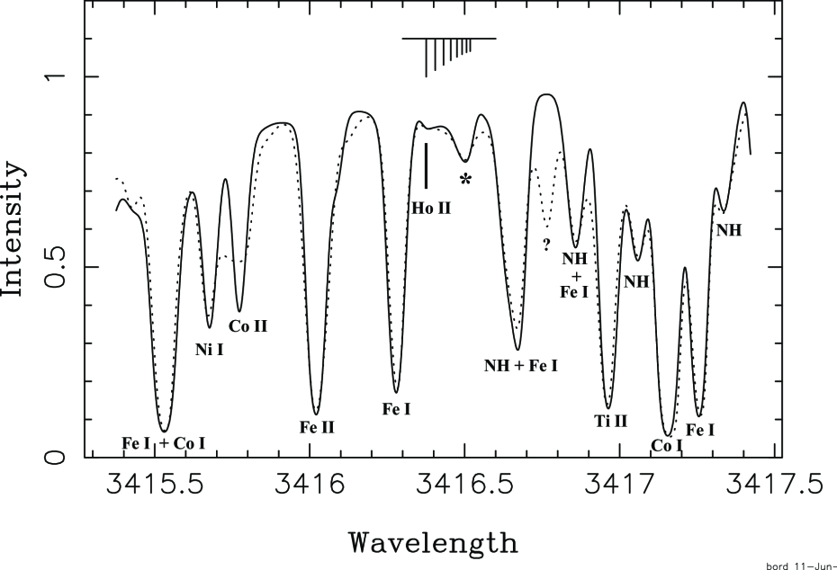
Figure 2: Synthesis (solid line) of the $\lambda 3416.4$ region of the solar spectrum with an adopted holmium abundance of +0.53 on the usual scale where log(H) = 12.00. The observations are again given by the dotted curve. The primary octet pattern in the hfs for the Ho II feature is also shown. The fit also reflects modifications in the positions and oscillator strengths of Ti I and Cr I lines near 3416.5 Å (asterisk symbol) as described in the text to better model the unidentified absorption (cf. Figure 1) immediately to the red of the Ho II line of interest. All other identifications follow Figure 1.

Figure 2 shows our synthesis (solid line) of this region for log(Ho) = +0.53. The observations are again given by the dotted curve. The primary hyperfine pattern for the Ho II feature is shown, with intensities drawn approximately to scale. Although only the eight principal lines are given in the figure, all twenty-two have been included in the synthesis. As isotope 165 comprises 100% of naturally occurring holmium, no additional wavelength shifts due to isotope effects are neccessary. Gravitational redshift effects on the wavelength of this line have been ignored in the calculation. As may be seen, with this choice of holmium abundance, the weak solar feature at 3416.375 Å is accounted for in a respectable fashion. This figure also shows the effects of “mocking up” the unidentified absorption at $\lambda_{\odot}3416.51$ by adjusting the VALD parameters for the Cr I and Ti I lines as remarked upon above.

Figure 3: Detail of solar spectrum in the vicinity of the Ho II 3416.44 Å line. As in Figure 2, the heavy solid line is the computed spectrum for log(Ho)=+0.53, while the observed spectrum is dotted. The upper(lower) thin lines show synthetic calculations with the holmium abundance decreased(increased) by 0.1 dex. The fit is obviously poorer near the positions of the strongest hfs components for the augmented(decremented) spectrum. The primary hfs for the Ho II line is again shown for reference, and its influence of the structure of the unidentified absorption feature at 3416.51 Å is obvious.

Figure 3 highlights the wavelength region in the immediate vicinity of the Ho II line and shows the effects of small variations in the abundance of this element. In particular, the thin solid lines show the calculated spectrum with the holmium abundance increased (bottom curve) or decreased (upper curve) by 0.1 dex with respect to the value adopted in Figure 2. As may be seen, the fit is demonstrably poorer near the positions of the strongest hfs components for the augmented and decremented plots. By additional fine tuning, a slightly better fit to the observations than that afforded by the heavy solid line might be achieved, but, given our earlier comments regarding the formal errors in the computations attributable to uncertainties in the adopted model atmosphere and the atomic parameters, we did not see much profit in doing so. As it is, our nominal best-fit value for the solar holmium abundance falls within 0.02 dex of the meteoritic value reported by GS, while prior considerations persuade us that our result is accurate to $\pm 0.15$ dex at best. We are reassured, to some degree however, of the validity of our result by the agreement between the holmium abundance derived from our best fit to the solar spectrum and that found by simply correcting the estimate of DBG to account for improvements in the partition function for this ion.

5 Conclusions

Uncertainties in the spectrum synthesis not withstanding, the results presented herein lend credence to the view that the abundance of holmium in the Sun follows the pattern of other rare-earth elements in showing general agreement with the meteorites. In Figure 4 we plot the logarithmic CI abundances from the compilation of McDonough and Sun (1995) minus the solar abundances from GS (with some small modifications to reflect recent work on the light elements by Holweger (2001)). Because McDonough and Sun have not been involved with the reconciliation of solar and meteoritic abundances, they may be considered an independent source for the meteoritic values, which are, in any case, very close to those reported by GS. (For example, McDonough and Sun give the logarithmic abundance of holmium in the meteorites as +0.49, 0.02 dex lower than the value quoted by GS but within the latter’s stated error.) The abundance differences are plotted versus elemental condensation temperatures taken from Lodders and Fegley (1998).

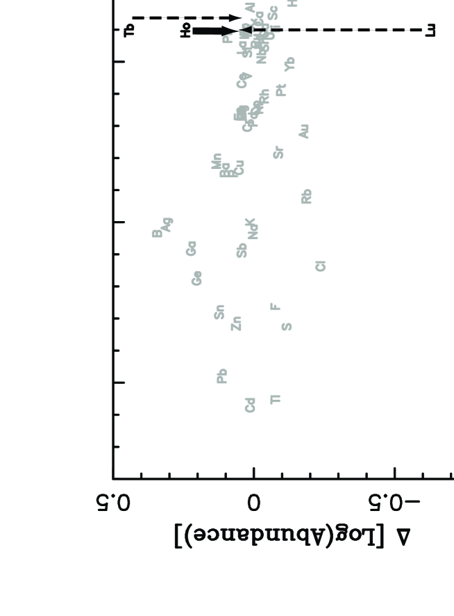
Figure 4: Logarithmic CI minus solar photospheric abundances vs. elemental condensation temperatures. Points are indicated by the chemical symbols of the elements. The position of holmium prior to and after the present work is shown by the heavy arrow. Recent adjustments in the abundances of lutetium and terbium are shown by the dashed arrows. Among the heavy and rare-earth elements, only tungsten (W) remains seriously discordant.

As may be seen in Figure 4, with recent revisions to the solar abundances of lutetium (Bord, Cowley, and Mirijanian, 1998), terbium (Lawler, et al., 2001) and now holmium, among the heavy and rare-earth elements, only tungsten remains seriously anomalous. The authors are currently investigating the prospects of being able to improve the photospheric abundance of this element using the techniques described in this paper.

Among the volatile elements, indium ($Z=49$) presents the greatest discordance. We have recently re-evaluated the solar abundance of this element in a manner similar to that described in this paper (cf. Bord and Cowley, 2001). Specifically, we synthesized a 2.25 Å segment of the solar spectrum centered on the position of the resonance line of In I at $\lambda 4511.3$. The hfs constants were taken from Jackson (1957, 1958), and the VALD log($gf$) = $-0.210$ was adopted. Our best fit to the solar data yielded log(In) = 1.56. This is about 0.1 dex smaller than the value found by Lambert, Mallia, and Warner (1969), the difference arising almost entirely from revisions in the oscillator strength of the line. We estimate that the formal errors in the computation are at least $\pm 0.2$ dex, half of which is due to residual uncertainties in the oscillator strength. The remainder of the error is contributed by uncertainties associated with the placement of the continuum which amount to about 1% in this region. We have thus confirmed that the Sun is overabundant in indium by a factor of more than 5, with log(In_CI)$-$log(In_⊙) $=-0.74$.

This difference is reflected in Figure 4 and remains a challenge to our understanding. With no other unblended indium lines available, further refinements in the solar abundance of this element appear remote. Moreover, the meteoritic abundance rests on 24 separate analyses made at three different labs and is uncertain by only 6% (Anders and Ebihara, 1982). Given that indium should be one of the last of the chalcophiles to leave the gas phase, conditions in the solar nebula may have led to its incomplete condensation and to a depletion of this species in the CI meteorites. If this were to be the case, one might expect to see a similar depletion of cadmium ($Z=48$) in these meteorites relative to the Sun. However, the cadmium abundance in the CI meteorites is within 0.01 dex of that found for the solar photosphere (Youssef, Dönszelmann, and Grevesse, 1990), so the mystery persists.

These exceptions not withstanding, it is quite remarkable - indeed, puzzling perhaps - the degree to which the abundances of the CI meteorites agree with those of the solar photosphere. Given the complex chemical histories of these meteorites in which aqueous alteration has likely played a significant role, it is surprising that the bulk atomic compositions of these bodies seem to have remained largely unfractionated. Continuing efforts to refine the abundances of trace elements in the Sun to permit more precise comparisons between the abundance patterns in our star and these meteorites hold promise for providing greater insight into the history of both.

- [1] Anders, E., and Ebihara, M.: 1982, Geochem. Cosmochem. Acta 46, 2363.
- [2] Bolton, C. T.: 1970, Astrophys. J. 161, 1187.
- [3] Bord, D. J.: 2000, Astron. Astrophys. Suppl. 114, 517.
- [4] Bord, D. J., and Cowley, C. R.: 2001, Bull. Amer. Astron. Soc. 33(4), 1433.
- [5] Bord, D. J., Cowley, C. R., and Mirijanian, D.: 1998, Solar Phys. 178, 221.
- [6] Brazier, C. R., Ram, R. S., and Bernath, P. F.: 1986, J. Mol. Spectr. 120, 381.
- [7] Brewer, L.: 1971, J. Opt. Soc. Amer. 61, 1666.
- [8] Cowan, R. D.: 1981, The Theory of Atomic Structure and Spectra (Berkeley: Univ. California Press).
- [9] Cowan, R. D.: 1995, Programs RCN/RCN2/RCG/RCE, Los Alamos National Laboratory (May 1995).
- [10] Cowley, C. R.: 1984, Physica Scripta T8, 28.
- [11] Cowley, C. R.: 1996, in S. J. Adelman, F. Kupka, and W. W. Weiss (eds.), Model Atmospheres and Spectrum Synthesis: 5th Vienna Workshop (San Francisco, CA: Astron. Soc. Pacific), p. 170.
- [12] Cowley, C. R., and Barisciano, Jr., L. P.: 1994, The Observatory 114, 308.
- [13] Daems, R., Biémont, E., and Grevesse, N.: 1984, unpublished results. (DBG)
- [14] Delbouille, L., and Roland, G.: 1995, in A. J. Sauval, R. Blomme, and N. Grevesse (eds.), Laboratory and Astronomical High Resolution Spectra, ASP Conf. Series, Vol. 81, p. 32.
- [15] Gorshkov, V. N., and Komarovskii, V. A.: 1979, Opt. Spectrosc. (USSR) 47, 350.
- [16] Grevesse, N.: 1984, Physica Scripta T8, 49.
- [17] Grevesse, N., and Blanquet, G.: 1969, Solar Phys. 8, 5. (GB)
- [18] Grevesse, N., and Sauval, A. J.: 1998, Space Sci. Rev. 85, 161. (GS)
- [19] Holweger, H.: 2001, in R. F. Wimmer-Schweingruber (ed.), Solar and Galactic Composition, ASP Conf. Series, in press.
- [20] Holweger, H., and Müller, E. A.: 1974, Solar Phys. 39, 19.
- [21] Jackson, D. A.: 1957, Proc. R. Soc. A241, 283.
- [22] Jackson, D. A.: 1958, Proc. R. Soc. A246, 344.
- [23] Kupka, F., Piskunov, N. E., Ryabchikova, T. A., Stempels, H. C., and Weiss, W. W.: 1999, Astron. Astrophys. Suppl. 138, 199.
- [24] Kurucz, R. L.: 1993, CD-ROM Nos. 15 and 18 (Cambridge, MA: Smithsonian Astrophys. Obs.).
- [25] Lambert, D. L., Mallia, E. A., and Warner, B.: 1969, Mon. Not. R. Astr. Soc. 142, 71.
- [26] Lawler, J. E., Wickliffe, M. E., Cowley, C. R., and Sneden, C.: 2001, Astrophys. J. Suppl. 137, 341.
- [27] Lodders, K., and Fegley, Jr., B.: 1998, The Planetary Scientist’s Companion (Oxford: Oxford Univ. Press), p. 83ff.
- [28] Martin, W. C., Zalubas, R., and Hagan, L.: 1978, Atomic Energy Levels–The Rare Earth Elements, NSRDS-NBS 60 (Washington: U. S. Gov. Print. Off.). (MZH)
- [29] McDonough, W. F., and Sun, S.-S.: 1995, Chem. Geol. 120, 223.
- [30] Meggers, W. F., Corliss, C. H., and Scribner, B. F.: 1975, Tables of Spectral Line Intensities, Part I, NBS Monograph 145 (Washington: U. S. Gov. Print. Off.).
- [31] Moore, C. E., Minnaert, M. G. J., and Houtgast, J.: 1966, The Solar Spectrum 2935Å to 8770Å, N.B.S. Monograph 61 (Washington: U. S. Gov. Print. Off.). (MMH)
- [32] Nave, G., Johansson, S., Learner, R. C. M., Thorne, A. P., and Brault, J. W.: 1994, Astrophys. J. Suppl. 94, 221.
- [33] Neckel, H.: 1999, Solar Phys. 184, 421.
- [34] Neckel, H., and Labs, D.: 1984, Solar Phys. 90, 205.
- [35] Radziemski, L. J., and Mack, J. M.: 1980, Physica 102B, 35.
- [36] Sneden, C., McWilliam, A., Preston, G. W., Cowan, J. J., Burris, D. L., and Armosky, B. J.: 1996, Astrophys. J. 467, 819.
- [37] Sugar, J.: 1968, J. Opt. Soc. Am. 58. 1519.
- [38] Worm, T., Shi, P., and Poulsen, O.: 1990, Phys. Scripta 42, 569.
- [39] Wyart, J.-F., Koot, J. J. A., and van Kleef, T. A. M.: 1974, Physica (Utrecht) 77, 159.
- [40] Youssef, N. H., Dönszelmann, A., and Grevesse, N.: 1990, Astron. Astrophys. 239, 367.
- [41] Zhang, Z. G., Svanberg, S., Palmeri, P., Quinet, P., and Biémont, E.: 2002, Astron. Astrophys. 385, 724.