Return mapping of phases and the analysis of the gravitational clustering hierarchy

Abstract

In the standard paradigm for cosmological structure formation, clustering develops from initially random-phase (Gaussian) density fluctuations in the early Universe by a process of gravitational instability. The later, non-linear stages of this process involve Fourier mode-mode interactions that result in a complex pattern of non-random phases. We present a novel mapping technique that reveals mode coupling induced by this form of nonlinear interaction and allows it to be quantified statistically. The phase mapping technique circumvents the difficulty of the circular characteristic of $\phi_{\mbox{\boldmath$k$}}$ and illustrates the statistical significance of phase difference at the same time. This generalized method on phases allows us to detect weak coupling of phases on any $\Delta{\mbox{\boldmath$k$}}$ scales.

1 Introduction

The morphology of the large-scale structure in the Universe is that of a complex hierarchy of nodes, filaments and sheets interlocking large voids. The Fourier-space description of such a pattern is dominated by the properties of the phases rather than the amplitudes of the Fourier modes [Chiang 2001]. According to the prevailing theoretical ideas this pattern developed by a process of gravitational instability from an amorphous pattern of density fluctuations characterized by a Gaussian field with random phases. Since the non-random phases of the present structure have grown from random-phase initial perturbations then there is strong motivation for understanding how phase information develops within this paradigm and to construct a statistical description of galaxy clustering that could be used as a test of the basic idea.

Unfortunately, quantifying the properties of Fourier phases is difficult for a number of technical reasons, so their use in statistical studies has so far been limited. Ryden & Gramann (1991), Soda & Suto (1992) and Jain & Bertschinger (1996) focused on the evolution of individual phases away from their initial values but since the initial phases are unknown these studies can not be used as the basis of a statistical descriptor. The pattern of association between phases is subtle and hard to visualize which makes a statistical test hard to construct a priori.

As the first step in a different approach towards quantifying phase information, Coles & Chiang (2000) proposed a colour representation method to visualize phase coupling that at least reveals qualitatively how phase information arises during the evolution of $N$-body experiments but does not in itself constitute a statistical descriptor. In a related study, Chiang & Coles (2000) quantified phase information using a statistic derived from the Shannon entropy of the distribution of successive phase differences. This study displayed interesting relationships between phase entropy and gravitational clustering but still did not provide a general statistical description.

In this paper we use a generalization of the concept of a return map [May 1976, Chiang & Coles 2000] to transfer the phases of different Fourier modes on to a bounded square upon which simple statistical tests can be applied. In this way, we build upon the earlier studies [Chiang & Coles 2000, Coles & Chiang 2000] to construct a method that allows us to transform the phase information in a clustering pattern into a more useful form.

2 Phase Coupling in the Nonlinear Regime

The mathematical description of an inhomogeneous Universe revolves around the dimensionless density contrast, $\delta({\mbox{\boldmath$x$}})$, which is obtained from the spatially-varying matter density $\rho({\mbox{\boldmath$x$}})$ via

$$\delta({\mbox{\boldmath$x$}})=\frac{\rho({\mbox{\boldmath$x$}})-\rho_{0}}{\rho_{0}},$$ (1)

where $\rho_{0}$ is the global mean density. When the density perturbation is small, the evolution of the density contrast can be obtained analytically through linear perturbation theory from 3 coupled partial differential equations. They are the linearized continuity equation,

$${\partial\delta\over\partial t}=-{1\over a}{\mbox{\boldmath$\nabla$}_{x}}\cdot{\mbox{\boldmath$v$}},$$ (2)

the linearized Euler equation

$${\partial{\mbox{\boldmath$v$}}\over\partial t}+{\dot{a}\over a}{\mbox{\boldmath$v$}}=-{1\over\rho a}{\mbox{\boldmath$\nabla$}_{x}}p-{1\over a}{\mbox{\boldmath$\nabla$}_{x}}\phi,$$ (3)

and the linearized Poisson equation

$${\mbox{\boldmath$\nabla$}_{x}}^{2}\phi=4\pi Ga^{2}\rho_{0}\delta.$$ (4)

In these equations, $a$ is the expansion factor, $p$ is the pressure, ${\mbox{\boldmath$\nabla$}_{x}}$ denotes a derivative with respect to the comoving coordinates $x$, ${\mbox{\boldmath$v$}}=a\dot{\mbox{\boldmath$x$}}$ is the peculiar velocity and $\phi({\mbox{\boldmath$x$}},t)$ is the peculiar gravitational potential. From Eq. (2)-(4), and if one ignores pressure forces, it is easy to obtain an equation for the evolution of $\delta$:

$$\ddot{\delta}+2(\frac{\dot{a}}{a})\delta-4\pi G\rho_{0}\delta=0.$$ (5)

For a spatially flat universe dominated by pressureless matter, $\rho_{0}(t)=1/6\pi Gt^{2}$ and Eq. (5) admits two linearly independent power law solutions $\delta({\mbox{\boldmath$x$}},t)=b_{\pm}(t)\delta_{0}({\mbox{\boldmath$x$}})$, where $\delta_{0}({\mbox{\boldmath$x$}})$ is the initial condition, $b_{+}(t)\propto a(t)\propto t^{2/3}$ is the growing mode and $b_{-}(t)\propto t^{-1}$ is the decaying mode.

It is useful to expand the density contrast in Fourier series, in which $\delta$ is treated as a superposition of plane waves:

$$\delta({\mbox{\boldmath$x$}})=\sum\tilde{\delta}({\mbox{\boldmath$k$}})\exp(i{\mbox{\boldmath$k$}}\cdot{\mbox{\boldmath$x$}}).$$ (6)

The Fourier transform $\tilde{\delta}({\mbox{\boldmath$k$}})$ is complex and therefore possesses both amplitude $|\tilde{\delta}({\mbox{\boldmath$k$}})|$ and phase $\phi_{\mbox{\boldmath$k$}}$ where

$$\tilde{\delta}({\mbox{\boldmath$k$}})=|\tilde{\delta}({\mbox{\boldmath$k$}})|\exp(i\phi_{\mbox{\boldmath$k$}}).$$ (7)

In the standard picture of ‘gravitational instability’ model for the origin of cosmic structure, particularly those involving inflation, the initial perturbations are Gaussian [Bardeen et al. 1986]. The most relevant property of Gaussian random fields is that they possess Fourier modes whose real and imaginary parts are independently distributed. In other words, they have phase angles $\phi_{\mbox{\boldmath$k$}}$ that are independently distributed and uniformly random on the interval $[0,2\pi]$. Terms in the perturbative evolution equations for the Fourier modes that represent coupling between different waves are of second (or higher) order in $\delta$ and these are neglected in linear perturbation theory. When fluctuations are small, i.e., during the linear regime, the Fourier modes evolve independently (Eq.( 5) and (6)) and the Gaussian character is retained in the linear regime, where the phases remain independent and uniformly random. In the later stages of evolution, however, modes begin to couple together. In this non-linear regime that Fourier phases become non-random. For a thorough review of the theory and implications of non-linear evolution from the point of view of perturbation theory, see Bernardeau et al. (2002).

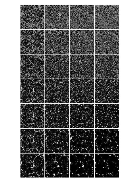
Figure 1: 2D $N$-body simulations for initial power spectral index, from left to right, $n=-1$, 0, 1 and 2, respectively. We choose 7 stages, named stage 1 to 7 from top to bottom, with an increasing level of non-linearity as described in the text. We control the simulations by setting the same initial random phase configuration for each index. Consequently, it is easy to see that the evolving structures have density concentration at the same locations; the difference is due to the initial spectral index: large $n$ will produce more clumps, small $n$ will have filaments.

Standard methods of analysis proceed via the power-spectrum, $P(k)$, essentially proportional to $|\tilde{\delta}({\mbox{\boldmath$k$}})|^{2}$. The probabilistic properties of Gaussian random fields are completely specified by knowledge of $P(k)$. Higher-order quantities based on $\tilde{\delta}({\mbox{\boldmath$k$}})$ can also be defined, such as the bispectrum [Peebles 1980, Matarrese, Verde & Heavens 1997, Scoccimarro et al. 1998, Scoccimarro, Couchman & Frieman 1999, Verde et al. 2000, Verde et al. 2001, Verde et al. 2002], which vanishes for Gaussian fields, or quantities related to correlations of $|\tilde{\delta}({\mbox{\boldmath$k$}})|^{2}$ [Stirling & Peacock 1996]. Phase coupling results in a non-Gaussian field in which the bispectrum and higher-order polyspectra may be non-zero [Watts & Coles 2002]. Phase information is at the heart of non-linear galaxy clustering.

Figure 2: Phase mapping onto the return map. The horizontal and vertical axes represent $\phi_{\mbox{\boldmath$k$}}$ and $\phi_{{\mbox{\boldmath$k$}}+\Delta{\mbox{\boldmath$k$}}}$, ranging from $0^{\circ}$ to $360^{\circ}$. In panel (a) the phases are taken from the stage 3, spectral index $n=1$ of the $N$-body simulations shown in Fig. 1 and the scale of phase mapping is $\Delta{\mbox{\boldmath$k$}}\equiv(m,n)=(0,33)$. The phases are condensed along the diagonal strip. Panels (b), (c) and (d) are the smoothed versions of various phase maps where the contour levels are drawn upwards starting from the mean value. Panel (b) is from a random-phase realization and (c) is that of stage 2, $n=1$. For comparison, both (b) and (c) are mapping from the same $\Delta{\mbox{\boldmath$k$}}$ scale $(m,n)=(-2,44)$. Panel (d) is the smoothed version of panel (a).

3 Directional Phase Mapping

There are two principal difficulties involved in constructing a statistic from Fourier phases. One is that because phases reflect the morphology, their values change according to the position of structural features [Chiang 2001]. For example, the phases of a peak in the form of Dirac-$\delta$ function $\delta_{D}(x-x_{0})$, $\phi_{k}=kx_{0}$ suffer change in slope along the $k$-axis when there is shift of the peak $\delta_{D}(x-x_{0}-x^{{}^{\prime}})$, the phases being $\phi_{k}=k(x_{0}+x^{{}^{\prime}})$. If a pattern is statistically homogeneous, any descriptor of it should be translation-invariant and this is manifestly not true of the phases themselves. The other problem is that phases are of circular measures and therefore defined modulo $2\pi$. Traditional measures of association, such as covariances of the form $\langle\phi_{i}\phi_{j}\rangle$, are based on the assumption that the measure associated with the variable is linear and are therefore not appropriate to cases where values separated by $2\pi$ are in fact equal in value.

To address these problems, Chiang & Coles (2000) used the phase difference (or phase gradient), $D_{k}$, defined in one dimension by

$$D_{k}\equiv\phi_{k+1}-\phi_{k},$$ (8)

i.e. for neighbouring phases. In two or three dimensions differences can be taken in orthogonal directions. The quantity $D_{k}$ has the twin advantages that for random phases it is also random but upon translation $x^{\prime}$ it changes by a constant $x^{\prime}$ for all $k$. The statistical properties of the set of differences $D_{k}$ contain information about the correlations of neighbouring Fourier modes. Strong correlation of the neighbouring modes at large $k$ corresponds to the highest peak in the clustering pattern. Naselsky, Novikov and Silk (2002) used this characteristic to extract point sources in the CMB map. Moreover, Chiang et al. (2001) used the phase analysis for extracting the in-flight beam shape properties of CMB experiments. To construct a more general description of phase coupling we need to extend this method to modes that are not necessarily neighbours. We do this by constructing a directional phase map, based on the return maps used in non-linear dynamics [May 1976].

The basic idea is simple and based on a study of one-dimensional examples contained in Chiang & Coles (2000) which provides a useful illustration of the more general approach. With a set of phases $\phi_{k}$ from the Fourier transform of a one-dimensional process, one can plot a map of $\phi_{k}$ against $\phi_{k+1}$ for each pair $(\phi_{k},\phi_{k+1})$. If the phases are random this will be a scatter plot with points distributed randomly within the bounded square of side $[0,2\pi]$. If there is association between neighbouring phases the plot will contain correlations; the quantity $D_{k}$ is sensitive to linear association. If the spatial pattern consists of a single high-amplitude peak the points display linear association and are mapped into a diagonal lines on the diagram.

Figure 3: The $\overline{\chi^{2}}$ statistics on grey scale for different realisations on the $(m,n)$ plane. The 4 panels correspond to the 4 realisations of Fig. 1, stage 2, 3, 4 and 5, spectral index $n=1$ of the 2D $N$-body simulations. In order to show clearly the maximal points, we set the same grey scale for panel (a), (b) and (c), and note that the grey scale of (d) is different. The maximal $\overline{\chi^{2}}$ for stage 2 is $2.53\times 10^{-2}$ at $(m,n)=(-2,44)$, and $3.27\times 10^{-2}$ for stage 3 at $(m,n)=(0,33)$, both mapping of the particular scale being shown in Fig. 2 (c) and (d). For panel (c) and (d) the $\overline{\chi^{2}}_{\max}=4.90\times 10^{-2}$ and $1.17\times 10^{-1}$ at $(m,n)=(12,5)$ and $(-4,8)$, respectively, which indicates the scale of phase coupling in the highly non-linear regime is at small $\Delta{\mbox{\boldmath$k$}}$.

In what follows, for illustration, we shall use two-dimensional examples based on numerical simulations with periodic boundaries, so we take $\Delta{\mbox{\boldmath$k$}}\equiv(m,n)$ where $m$ and $n$ are integers. The simulations are done on a $512^{2}$ grid. In Fig. 1 we show 4 sets of such $N$–body simulations for initial power spectral index $n=-1$, 0, 1 and 2 (see Chiang & Coles 2000 for details of the simulations). The evolutionary stages are characterized by an increasing scale of non-linearity defined by $\left<\left(\delta\rho/\rho\right)^{2}\right>_{k_{\rm NL}}=b^{2}_{+}(t)\int^{k_{\rm NL}}_{0}P(k)\>d^{2}k=1$, where $b_{+}(t)$ is the growing mode of the linear density contrast and $P(k)$ is the linear extrapolation of the initial power spectrum. This definition of $k_{\rm NL}$ identifies the corresponding scale $2\pi k_{\rm NL}^{-1}$ as the boundary between linearity and non-linearity. The stages in Fig. 1 are chosen such that the scales of non-linearity $k_{\rm NL}$ between any two successive stages vary by a factor of 2. The levels of non-linearity of the stages are thus $k_{\rm NL}=256$, 128, 64, 32, 16, 8 and 4.

We can use these simulations to illustrate how we extend the return mapping between neighbouring phases ($\Delta{\mbox{\boldmath$k$}}=1$) to pairs of phases with any $\Delta{\mbox{\boldmath$k$}}$ scales in $k$-space. We map all pairs of phases $\phi(i,j)$ and $\phi(i+m,j+n)$ onto the $x$ and $y$ values of the return map. The axes therefore range over $[0,2\pi]$ for both $\phi({\mbox{\boldmath$k$}})$ ($x$) and $\phi({\mbox{\boldmath$k$}}+\Delta{\mbox{\boldmath$k$}})$ ($y$) axes. For example, for $(m,n)=(4,6)$ we have points on the return map $(\phi(i,j),\phi(i+4,j+6))$ for all $i\in[-255,256]$, $j\in[1,256]$, i.e., all points $(\phi(1,1),\phi(5,7))$, $(\phi(2,1),\phi(6,7))$, $(\phi(1,2),\phi(5,8))\ldots$, from a 2D Fourier transform of a realisation. This represents the directional phase coupling for coupling scale $\Delta{\mbox{\boldmath$k$}}\equiv(\Delta k_{x},\Delta k_{y})\equiv(m,n)$ in $k$-space. The neighbouring phase differences in the $k_{x}$-direction and $k_{y}$-direction used by Chiang & Coles (2000) simply corresponds to $(m,n)=(1,0)$ and $(0,1)$ respectively.

In Fig. 2 (a) we show one example of phase mapping from the realization of stage 3, spectral index $n=1$ simulation. The particular $\Delta{\mbox{\boldmath$k$}}$ in this example is $(m,n)=(0,33)$. This panel demonstrates how weak coupling between phase pairs with fixed scale $\Delta{\mbox{\boldmath$k$}}$ can manifest itself in the return map as non-uniform density in the map plane.

This directional phase mapping approach circumvents the problem of the circular character of $\phi_{\mbox{\boldmath$k$}}$ but does not attempt to condense all the related information into a single quantity. It, on the other hand, exploits all the information between all Fourier modes. For example, the phase coupling of a 1D distribution can be expressed in a (2D) return map. It therefore allows us to build simple statistics to test the significance of general non-randomness. The phase difference between any pair at a fixed scale becomes a single point on the return map for that scale. The circular characteristic of $\phi_{\mbox{\boldmath$k$}}$ is transferred to a bounded square, topologically equivalent to a torus owing to the periodicity of $x$ and $y$ axes. The bands seen in Fig. 2 (a) therefore correspond to twisted linear features on this torus.

The key advantage of directional phase mapping is that, for a Gaussian random field, any directional phase mapping for any scale $\Delta{\mbox{\boldmath$k$}}\equiv(m,n)$ should produce a random Poisson distribution. Weak phase coupling will produce correlations at large vectors $(m,n)$ while strong non-linearity will produce highly non-uniform phase maps at all scales $(m,n)$.

4 A $\chi^{2}$ Test on Phase Maps

Once we have transferred the phase information onto a phase map like that shown in Fig. 2 (a), many different statistical tests can be used to analyse its properties. Here we outline a simple yet powerful method.

First we smooth the return map. Smoothing enhances our visualization of the pattern of phase coupling. In Fig. 2 (b), (c), and (d) we show the contour maps of the smoothed return map. In these simple illustrative experiments we divide the square of the return map into $128^{2}$ pixels, and we bin the 32 768 points so that, for a perfectly even distribution in the map plane the occupation of each pixel is $\langle p(i,j)\rangle=2$. Then we smooth this $128^{2}$ mesh by

$$p({\mbox{\boldmath$x$}},R)=(\sqrt{2\pi}R)^{-2}\int d^{2}{\mbox{\boldmath$x$}^{{}^{\prime}}}\>p({\mbox{\boldmath$x$}^{{}^{\prime}}})\>\exp\left(-\frac{|{\mbox{\boldmath$x$}}-{\mbox{\boldmath$x$}^{{}^{\prime}}}|^{2}}{2R^{2}}\right).$$ (9)

The contour levels are drawn upwards starting from the mean value. Panel (b) is the contour of a smoothed return map from a realization of random phases. Panel (c) is that from stage 2, $n=1$ of Fig. 1 with $(m,n)=(-2,44)$. For comparison, the coupling scale $\Delta{\mbox{\boldmath$k$}}$ for both (b) and (c) is set the same. We can see that even for the mildly non-linear regime represented by stage 2 (for which $\delta\simeq 1.8$), phase mapping does reveal the existence of coupling by starting to condense on the diagonal strip. Panel (d) is the smoothed version of (a) with $(m,n)=(0,33)$, in which the condensed strip from (a) is much clearer.

We define a mean $\chi^{2}$ statistic as

$$\overline{\chi^{2}}=\frac{1}{M}\sum_{i,j}\frac{\big{[}p(i,j)-\overline{p}\big{]}^{2}}{\overline{p}}$$ (10)

where $M$ is the number of pixels we assign on the return map and $\overline{p}$ is the mean value for each pixel.

In Fig. 2, the smoothing scale on the $128^{2}$ mesh is $R=2$ and the contour levels are drawn starting from the mean value. We use this pixel size and smoothing scale in all our calculations of $\overline{\chi^{2}}$ in the following, but one can vary the scale as part of a statistical test.

5 Simulation Results

We now illustrate the results of this analysis using the 2D $N$-body simulations described earlier. First we Fourier transform the realizations of the $N^{2}$ mesh ($N=512$ in our simulations). Because of the reality of the original distribution, and the consequent Hermitian conjugate relations in the Fourier image, only half of the Fourier transform contains independent information. We end up with $N^{2}/2$ Fourier modes available, so we take $-k_{N/2}+1$ to $k_{N/2}$ in $k_{x}$ axis and from 1 to $k_{N/2}$ in $k_{y}$ axis.

Figure 4: The maximal $\overline{\chi^{2}}$ is plotted against 1D Fourier scale $|\Delta{\mbox{\boldmath$k$}}|\equiv\sqrt{m^{2}+n^{2}}$ for stage 2 and 3 of simulations from initial spectral index $n=-1$, 0, 1 and 2. The maxima are taken from each $|\Delta{\mbox{\boldmath$k$}}|$ ring of the $(m,n)$ plane.

We carry out a phase mapping for each $(m,n)$. The directional phase mapping is performed for the vectors $(m,n)$, where $m\in[-49,50]$ and $n\in[1,50]$ for the phase base $\phi(i,j)$, where $i\in[-127,128]$, and $j\in[1,128]$, a quarter of the available phases. The limited range of mapping vectors is chosen to ensure that the map can be constructed without running out of sensible wavenumbers. Thus, in such a case, for each return map of $(m,n)$ there are $2\times 128^{2}$ points. We set up $M=128^{2}$ pixels in this $[0,2\pi]$ square and then smooth the return map to decrease the fluctuation. The $\overline{\chi^{2}}(m,n)$ for each fixed scale $(m,n)$ is calculated by Eq. (10).

Figure 3 shows ‘supermaps’ of all the phase information contained in the $\overline{\chi^{2}}(m,n)$ using a grey scale in the $(m,n)$ plane from various realisations of simulations. We are interested specifically on the mild non-linear regime, so in Fig. 3 the panels (a), (b), (c) and (d) correspond to stages 2, 3, 4 and 5 of $n=1$ in Fig. 1, respectively. The $m$-axis ranges from $-49$ to $50$ and $n$-axis ranges from 1 to 50. Each pixel therefore displays the level of phase coupling on a certain scale $(\Delta k_{x},\Delta k_{y})\equiv(m,n)$ in terms of the $\overline{\chi^{2}}$ statistics. The bright points in Figure 3 are direct indications of phase coupling for the corresponding $\Delta{\mbox{\boldmath$k$}}$ scales.

Figure 5: The maximal $\overline{\chi^{2}}$ is plotted against 1D Fourier scales $|\Delta{\mbox{\boldmath$k$}}|\equiv\sqrt{m^{2}+n^{2}}$ for stage 4 and 5 of simulations from initial spectral index $n=-1$, 0, 1 and 2. The maxima are taken from each $|\Delta{\mbox{\boldmath$k$}}|$ ring of the $(m,n)$ plane.

The reason we present the specific scales $(m,n)=(-2,44)$ for stage 2 and $(m,n)=(0,33)$ for stage 3, $n=1$ in Fig. 2 is that the calculation of the $\overline{\chi^{2}}$ statistics shows them to be ‘hotspots’ of phase correlation. The scales of phase coupling for those two panels correspond to the brightest points, i.e. the maximum $\overline{\chi^{2}}$ on the corresponding $(m,n)$ planes in Fig. 3.

In Fig. 4, 5 and 6 we plot the maximum $\overline{\chi^{2}}$ against $|\Delta{\mbox{\boldmath$k$}}|$ for all 4 sets of simulations. These 1D plots show that the maximal phase coupling from each ring $|\Delta{\mbox{\boldmath$k$}}|\equiv\sqrt{m^{2}+n^{2}}$ of the $(m,n)$ plane. As we control the simulations by assigning the same set of initial random phases, These 1D plots will display how the scale $|\Delta{\mbox{\boldmath$k$}}|$ of phase coupling is related to morphology.

The $N$-body simulations we have carried out is of self-similar nature, that is, a distribution function $f({\mbox{\boldmath$x$}},t)$ has the same statistical measure as the re-scaled one

$$f\mapsto\lambda^{\alpha}f({\mbox{\boldmath$x$}}/\lambda^{\beta},\lambda t),\mbox{ as $t\mapsto\lambda t$}.$$ (11)

With the reciprocal-scaling property of Fourier transform,

$$f(\alpha{\mbox{\boldmath$x$}})=\frac{1}{|\alpha|}F\left(\frac{\mbox{\boldmath$k$}}{\alpha}\right),$$ (12)

for non-linear scales ${\mbox{\boldmath$x$}}_{\rm NL}$ increasing, i.e. $\alpha>1$, the corresponding scales in $k$ space are decreasing. Although phases do not possess a linear relationship owing to their circular nature, it can be understood qualitatively that, if there exists coupling between pairs of phases with fixed $\Delta{\mbox{\boldmath$k$}}$, this scale has to decrease as gravitational clustering proceeds.

Figure 6: The maximal $\overline{\chi^{2}}$ is plotted against 1D Fourier scales $|\Delta{\mbox{\boldmath$k$}}|\equiv\sqrt{m^{2}+n^{2}}$ for stage 6 and 7 of simulations from initial spectral index $n=-1$, 0, 1 and 2. The maxima are taken from each $|\Delta{\mbox{\boldmath$k$}}|$ ring of the $(m,n)$ plane. Note that the scale of $y$-axis is 10 times larger than that in Fig. 4 and 5.

It is therefore clear that for the case such as $n=-1$, where large-scale filaments are the prominent feature, phase coupling starts from low $\Delta{\mbox{\boldmath$k$}}$, which also has cascade effect on to higher $\Delta{\mbox{\boldmath$k$}}$, as phases strongly couple on any $\Delta{\mbox{\boldmath$k$}}$ might also do so at multiples of $\Delta{\mbox{\boldmath$k$}}$. For high $n$, on the other hand, where small clumps form first, phase coupling starts from large $\Delta{\mbox{\boldmath$k$}}$. This also explains why the Shannon entropy from neighbouring phase difference can produce considerable results at early stages for $n=-1$, but not for $n=2$ (see the fig.5 of Chiang & Coles 2000). On the other hand, the coupling between the amplitudes are enhanced by the factor $1/\alpha$ as clustering proceeds, so mode-mode coupling between amplitudes at early stages is not as obvious as between phases. For a discussion of how this relates to the development of phase correlations in mildly non-linear evolution, see Watts & Coles (2002).

The $\overline{\chi^{2}}$ statistics shown on the $(m,n)$ plane and those 1D plots confirm the visualization of phase coupling presented by Coles & Chiang (2000). Phase coupling firstly appears on large $\Delta{\mbox{\boldmath$k$}}$ when the the scale of non-linearity is small in real space, then it shifts on the $(m,n)$ plane to small $\Delta{\mbox{\boldmath$k$}}$ in Fig. 3 (c) and (d) and finally dominates at neighbouring modes as seen in Fig. 6.

6 Conclusion

We have generalized a method based on phase mapping on the return map. This simple, easy-to-implement method can detect phase coupling at any scales $\Delta{\mbox{\boldmath$k$}}$ in $k$ space. We apply this method to two-dimensional simulations of gravitational clustering and the result has shown that even when the evolution is in the mild non-linear regime, phase coupling on certain scale is revealed through the $\overline{\chi^{2}}$ statistics on the $(m,n)$ plane.

In contrast to other methods, such as the Shannon entropy of the distribution of neighbouring phase differences [Chiang & Coles 2000], this method does not require large number of phases. Moreover, this approach can detect the scale of phase coupling through the phase mapping as shown in Fig. 2.

With the systematic $N$-body simulations shown in Fig. 1, we have also demonstrated in Fig. 4-6 that the scale of phase coupling differs according to the clustering morphology: modes between small $\Delta{\mbox{\boldmath$k$}}$ for large-scale filaments, large for small clumps.

This method reveals a signature of non-linear gravitational instability, but also offers the opportunity to provide a general test of Gaussianity that could be applied to cosmic microwave background temperature maps. In future work we shall evaluate the effectiveness for such method.

References

- [Bardeen et al. 1986] Bardeen J.M., Bond J.R., Kaiser N., Szalay A.S., 1986, ApJ, 304, 15
- [Bernardeau et al. 2002] Bernardeau F., Colombi S., Gaztanaga E., Scoccimarro R., 2002, Phys. Rep., in press (astro-ph/0112551)
- [Chiang 2001] Chiang L.-Y., 2001, MNRAS, 325, 405
- [Chiang & Coles 2000] Chiang L.-Y., Coles P., 2000, MNRAS, 311, 809
- [Chiang et al. 2001] Chiang L.-Y. et al., 2001, A&A in press (astro-ph/0110139)
- [Coles & Chiang 2000] Coles P., Chiang L.-Y., 2000, Nat, 406, 376
- [Jain & Bertschinger 1996] Jain B., Bertschinger E., 1996, ApJ, 456, 43
- [Matarrese, Verde & Heavens 1997] Matarrese S., Verde L., Heavens A.F., 1997, MNRAS, 290, 651
- [May 1976] May R.M., 1976, Nat, 261, 459
- [Naselsky, Novikov & Silk 2000] Naselsky P.D., Novikov D.I., Silk J., 2002, ApJ, 655, 565
- [Peebles 1980] Peebles P.J.E., 1980, The Large-Scale Structure of the Universe, Princeton Univ. Press, Princeton, NJ
- [Ryden & Gramann 1991] Ryden B.S., Gramann M., 1991, ApJL, 383, L33
- [Scherrer, Melott & Shandarin 1991] Scherrer R.J., Melott A.L., Shandarin S.F., 1991, ApJ, 377, 29
- [Scoccimarro et al. 1998] Scoccimarro R., Colombi S., Fry J.N., Frieman J.A., Hivon E., Melott A.L., 1998, ApJ, 496, 586
- [Scoccimarro, Couchman & Frieman 1999] Scoccimarro R., Couchman H.M.P., Frieman J.A., 1999, ApJ, 517, 531
- [Soda & Suto 1992] Soda J., Suto Y., 1992, ApJ, 396, 379
- [Stirling & Peacock 1996] Stirling A.J., Peacock J.A., 1996, MNRAS, 283, L99
- [Verde et al. 2001] Verde L., Jimenez R., Kamionkowski M., Matarrese S., 2001, MNRAS, 325, 412
- [Verde et al. 2000] Verde L., Wang L., Heavens A.F., Kamionkowski M., 2000, MNRAS, 313, 141
- [Verde et al. 2002] Verde L. et al. 2002, MNRAS in press (astro-ph/0112161)
- [Watts & Coles 2002] Watts P.I.R., Coles P., 2002, MNRAS, submitted