On the Temperature Structure of M87

Abstract

We revisit the XMM-Newton observation of M87 focusing our attention on the temperature structure. We find that spectra for most regions of M87 can be adequately fit by single temperature models. Only in a few regions, which are cospatial with the E and SW radio arms, we find evidence of a second temperature. The cooler component (kT $\sim$ 0.8-1 keV) fills a small volume compared to the hotter component (kT $\sim$ 1.6-2.5 keV), it is confined to the radio arms rather than being associated with the potential well of the central cD and is probably structured in blobs with typical sizes smaller than a few 100 pc. Thermal conduction must be suppressed for the cool blobs to survive in the hotter ambient gas. Since the cool gas is observed only in those regions of M87 where we have evidence of radio halos our results favor models in which magnetic fields play a role in suppressing heat conduction. The entropy of the cool blobs is in general smaller than that of the hot phase gas thus cool blobs cannot originate from adiabatic evolution of hot phase gas entrained by buoyant radio bubbles, as suggested by Churazov et al. (2001). An exploration of alternative origins for the cool gas leads to unsatisfactory results.

1 Introduction

M87 is the giant elliptical galaxy at the center of the Virgo cluster. It is amongst the most studied objects in the sky. Observations at radio and X-ray wavelengths, over the past few years, have allowed us to improve substantially our understanding of the physical processes in this source. The ROSAT analysis of M87 (Böhringer et al. 1995) has shown excess emission correlated with the radio structure and that this emission originates from gas cooler than the surrounding intracluster medium. A detailed radio map of M87 obtained with the VLA at 90 cm (Owen et al. 2000) provided evidence for a very complex radio structure. The authors identified two “bubbles” of synchrotron emission located respectively E and SW some 20-30 kpc from the nucleus. The bubbles are most likely supplied with energy and relativistic plasma which come ultimately from the active nucleus and the inner jet of M87. Largely on the basis of the above X-ray and radio observations Churazov et al. (2001) have developed a model for M87. These authors propose that the bubbles discovered by Owen et al. (2000) buoyantly rise through the cluster atmosphere. During their rise the bubbles uplift relatively cool X-ray emitting gas from the central regions to larger distances. Since the entrained gas is cooler than the ambient gas, the radio bubbles are trailed by cool elongated X-ray features. From the analysis of the XMM-Newton observation of M87, Belsole et al. (2001) have shown that cospatially with the radio bubbles the X-ray emission can be modeled as the sum of two single temperature components, with temperatures of about 2 and 1 keV respectively. In a recent paper based on a Chandra observation of M87, Young et al. (2002) have confirmed the results reported by Belsole et al. (2001).

In this Letter we revisit the XMM-Newton observation, and also make some use of a Chandra observation of M87. We perform a detailed spectroscopic analysis with the aim of better constraining the temperature structure of M87 and consequently gain a deeper understanding of the physical processes at work in this source. The remainder of the paper is organized as follows. In Section 2 we briefly review the XMM-Newton observation and data preparation. In Section 3 we describe the spectral modeling of the M87 data. In Section 4 we focus on the cool component emission. Finally in Section 5 we summarize our main results.

2 Observations and Data Preparation

We use XMM-Newton EPIC data from the PV observation of M87/Virgo. Details on the observation, as well as results from the analysis of this object, have already been published in various papers including Böhringer et al. (2001), Belsole et al. (2001), Molendi & Pizzolato (2001), Molendi & Gastaldello (2001), Gastaldello & Molendi (2002) and Matsushita et al (2002).

We have obtained calibrated event files for the MOS1, MOS2 and pn cameras with SASv5.2. In this Letter we use pn data only for the imaging analysis described in Section 4, spectral analysis has been performed on MOS1 and MOS2 data. At the time of writing, the calibration of the MOS detector in the relevant energy range (0.4-4.0 keV) is better than that of the pn detector, moreover the superior spectral resolution of the MOS with respect to pn allows a better modeling of the line rich spectra observed in M87.

Data were manually screened to remove any remaining bright pixels or hot column. There have been no soft-proton flares during the M87 observation and consequently no rejection for time periods with high background has been applied. We have divided the M87 observation in 8 concentric annuli centered on the emission peak. Each ring has been further divided into sectors for a total of 107 regions.

Spectra have been accumulated for MOS1 and MOS2 independently. The Lockman hole observations have been used for the background. Periods in which the background is increased by soft-proton flares have been excluded using an intensity filter; we rejected all events accumulated when the count rate exceeds 15 cts/100s in the $[10-12]$ keV band. Background spectra have been accumulated from the same detector regions as the source spectra. The vignetting correction has been applied to the spectra rather than to the effective areas, similarly to what has been done by other authors who have analyzed EPIC data (e.g. Arnaud et al. 2001). Spectral fits were performed in the 0.4-4.0 keV band. Data below 0.4 keV were excluded to avoid residual calibration problems in the MOS response matrices at soft energies. Data above 4 keV were excluded because above this energy the spectra show a substantial contamination from hotter gas emitted farther out in the cluster, on the same line of sight.

3 Spectral Modeling

All spectral fitting has been performed using version 11.0.1 of the XSPEC package. All models discussed below include a multiplicative component to account for the galactic absorption on the line of sight of M87. The column density is always fixed at a value of 1.8$\times 10^{20}$ cm^-2, which has been determined from a detailed 21 cm measurement in the direction of M87 (Lieu et al. 1996). The above value is somewhat smaller than the one derived by Stark et al. (1992), 2.5$\times 10^{20}$ cm^-2, obtained at a lower spatial resolution. We note that such small variations in column density do not affect in any substantial way our results.

We have first compared our data with a single temperature model (vmekal model in XSPEC), which allows to fit separately individual metal abundances. This model has 14 free parameters: the temperature $T$, the normalization and the abundance of $N$, $O$, $Ne$, $Na$, $Mg$, $Al$, $Si$, $S$, $Ar$, $Ca$, $Fe$ and $Ni$, which are all expressed in solar units.

As shown in Gastaldello & Molendi (2002) using the apec rather than the mekal model yields very similar results as far as the temperature and the normalization are concerned. Since temperatures and normalizations are the quantities we are interested in we have not run the apec model on our data.

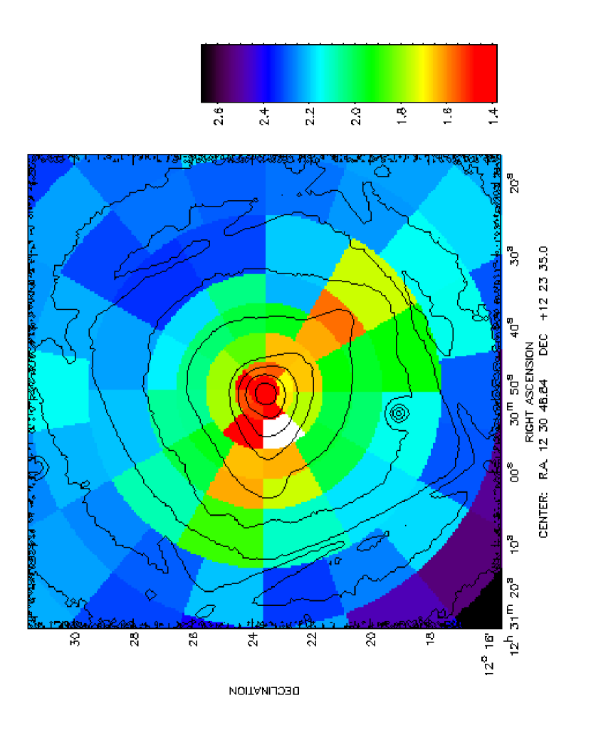
Figure 1: Temperature map, obtained from the 1 temperature run, overlaid on intensity contours. The color palette on the right shows the correspondence between colors and temperature expressed in keV. The white patch corresponds to a value slightly below 1.4 keV

In Figure 1 we show the temperature map obtained from the single temperature model run on the data. The map shows that in general the temperature is smaller at smaller radii. However the most interesting result is the presence of cooler regions which extend from the core in the E and SW directions. We will refer to these regions from now on as the E and SW “arms”. Our findings are in agreement with previous analysis of the XMM M87 observation by Belsole et al. (2001) and Matsushita et al. (2002).

We have then compared our data with a two temperature model (vmekal + vmekal model in XSPEC). This model has two free parameters more than the single temperature model: the temperature and the normalization of the second component. Since we are interested in the temperature structure we have chosen to link the metal abundance of the second component to that of the first component. From tests on sample spectra we have found that, with the exception of Fe, allowing the metal abundances of the two components to vary independently results in little difference in the normalizations and temperatures of the best fitting model. In the case of Fe there is a correlation between the normalization and the Fe abundance for the cooler component, because the spectral range where this component contributes most significantly to the observed spectra is around 0.8-1.0 keV where the cooler component emission is dominated by the Fe-L shell line blend. Tests on sample spectra show that the correlation between normalization and Fe abundance of the cooler component is such that, within the 90% confidence contours, the former can be reduced up to 30-50% if the latter is allowed to increase by a similar amount.

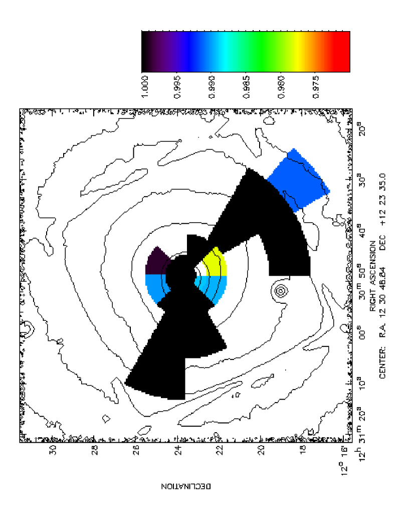
Figure 2: F-Probability map obtained by comparing the best fits of the 1 and 2 temperature runs, overlaid on intensity contours. The color palette on the right shows the correspondence between colors and probability values.

To establish if spectra are better represented by a 2 temperature model than by a 1 temperature model we have made use of the F-test. In Figure 2 we show the value of the probability, associated to the F-test, for the improvement to be statistically significant. Quite interestingly it is only for the two arms extending from the core in the E and SW directions that we have evidence of more than 1 temperature. For all other regions spectra are consistent with being emitted by a single-phase gas.

One possible way to test the robustness of our characterization of the cooler component is to take the spectrum from a region where we have evidence of two temperatures and subtract from this the spectrum of a nearby region at the same angular distance from the center of M87 showing no evidence of the cool component. Since, as detailed later on in this section, the hotter component does not feature strong azimuthal variations, we expect that the spectrum resulting from the above subtraction should be well represented by a single temperature model with temperature and normalization similar to those found for the cool component. We have conducted the above test on 4 sectors, some in the SW and others in the E arm, in all cases we find that the resulting spectra can be well fitted by a single temperature model with temperature and normalization differing no more than 10% from those previously derived from the two temperature fits of the same regions.

We note that the presence of a second temperature component in the E and SW arms was already discussed in the Matsushita et al. (2002) and Belsole et al. (2002) paper; the statistical test we conduct here firmly establishes that this second thermal component is found in the SW and E arms and nowhere else at a comparable statistical significance level.

In general the reduced $\chi^{2}$ we obtain from our 2 temperature fits indicate that this model provides a fair description of the data. There are three regions for which the probability associated to the $\chi^{2}$ is smaller than 0.01, visual inspection of the residuals shows that in all three cases an important contribution to the total $\chi^{2}$ comes from two spectral ranges: the first around 1.1-1.3 keV and the second around 1.7-1.9 keV range. Inspection of other spectra, where the fits are formally acceptable, indicates that residuals in the above energy ranges are rather common. For the 1.1-1.3 keV range the residuals may reflect an incomplete modeling of the Fe-L lines in the mekal code while for the 1.7-1.9 keV they are probably due to an insufficient modeling of the Si edge fine structure in the detector quantum efficiency.

We have fitted spectra showing evidence of a second thermal component with a 3 temperature model (vmekal + vmekal + vmekal model in XSPEC) and with a 2 temperature plus cooling-flow model (vmekal + vmekal + vmcflow in XSPEC). By making use of the F-test we find that the introduction of a third temperature or of a cooling-flow component does not provide a statistically significant improvement to the fit. Thus, from an observational point of view, our results on the temperature structure may be summarized as follows. For most regions the gas can be well described by a single temperature model. For the two arms extending respectively E and SW the spectra can be adequately described by a two temperature model. The lack of improvement in the fit when going to models more complicated than 2 temperatures does not mean that the gas is strictly composed of two phases and there is no emission at all at any other temperature. The correct way of interpreting our result is that the bulk of the emission is coming from gas with a temperature close to either one of the two temperatures found in our best fits. Emission from any other component is relatively small. To quantify the latter statement we have performed the following exercise on the sector with bounding radii 2^′ and 3^′ and bounding angles 150^o and 180^o (angles are counted starting from West and going counter clockwise), which is characterized by a particularly intense cool component. We have added a third temperature component to our two temperature model and frozen the temperatures of the first 2 components as well as the normalization of the hotter component to the best fitting values found from the 2T fit. We have then run fits stepping the temperature of the third component from 0.5 to 5 keV. For each fit we have derived the 90% confidence upper limit for the normalization of the third component. In Figure 3 we show the ratio of the 90% upper limit for the normalization of the third component over the cool component normalization as a function of the temperature of the third component. The plot nicely illustrates that a third component can contribute substantially with respect to the cool component measured in the two temperature fit, only if its temperature is larger than $\sim 0.8$ keV, emission from gas at temperatures smaller than 0.6 keV has an associated normalization that is no more than 2% of that of the cool component. Some emission from gas with temperatures in the range between 1.7 and 5 keV cannot be ruled out, the intensity of this emission can be relatively large if compared to that of the cool component, however it is much smaller (a few percent) when compared to that of the hot component.

In Figure 4 we report the “normalized” emission integrals (EI), i.e. the emission integrals, as derived by spectral fitting, divided by the area of the region over which they have been measured, as a function of radius (for more details see the Figure caption). For those sectors where we have evidence of two temperatures, we report the normalized EI of the hot and cool components while for all other sectors we plot the normalized EI obtained from the one temperature fit. Similarly in Figure 5 we report the temperatures as a function of radius, showing both hot and cool component temperatures for two temperature regions and the temperature obtained from the 1T fits for all other regions. We note that neither the normalized EIs nor the temperatures for the hot or single phase component show evidence of a large scatter at any given radius, indicating that no strong azimuthal gradients are present. Moreover for those annuli where we have 1 and 2 temperature measurements we find that the temperature and normalized EI of the hot component are not clearly separated from the temperature and normalized EI of the single temperature fits, as is to be expected if the hot component observed in the 2 temperature regions is essentially the same we measure in the 1 temperature regions. Thus the picture emerging from our analysis is that of a 2 temperature structure, with the hot component that is distributed in a regular and symmetric fashion and a cool component that is observed only in the SW and E arms. It is to this latter component that we now turn our attention.

4 The cool component

In a number of papers based on ASCA observations various authors (e.g. Ikebe et al. 1996, Makishima et al. 2001) have discussed 2 temperature models as an alternative to the multi-phase cooling-flow model preferred by other authors. In the two temperature model presented by the above authors the higher and lower temperature components are associated respectively to gas in the potential well of the cluster and of the cD galaxy. The potential would thus be characterized by a sort of hierarchical structure. From Figure 2 it is evident that the lower temperature component has a highly asymmetric distribution which is reminiscent of the radio emission (cfr. Owen et al. 2000) and is not associated to the cD which has a much more regular structure. Thus the EPIC observation provides evidence against a model in which the lower temperature component is associated to gas in the potential well of the cD galaxy.

We now wish to further investigate the nature of the cooler component, and more specifically to determine the volume occupied by this component with respect to that occupied by the hot component. For a given region this can be expressed as $V_{c}\sim EI_{c}/n_{c}^{2}$, where $V_{c}$ is the volume occupied by the cool component and $EI_{c}$ and $n_{c}$ are respectively the emission integral and gas density of the cool component. Note that the above estimate is valid under the assumption that the cool component is confined to a scale in projection comparable to the observed extent of the arms within the plane of the sky. To compute $V_{c}$ we need an estimate of $n_{c}$, which can be obtained by assuming that the hot and cool components are in pressure equilibrium with one another.

There are a number of reasons that favor pressure equilibrium between the various components: 1) the X-ray data does not show evidence of shocks anywhere in M87, which would be expected in the presence of substantial pressure jumps and/or supersonic motions; 2) radio observations (Owen et al. 2000) indicate that the radio bubbles are most likely not overpressurized with respect to the X-ray gas; 3) if strong pressure gradients were present between the hotter and cooler X-ray emitting gas and or the radio plasma they would be reduced on a few sound crossing timescales which, assuming a typical size of a few kpc would be smaller than $10^{7}$ yr. Finally we note that, as far as our calculations are concerned, we do not require exact pressure equilibrium. Indeed as we shall see below our conclusions would not change if the pressure of the hot and cool components were within a factor of 2 of each other.

Under the assumption of pressure equilibrium the volume occupied by the cool component can be expressed as $V_{c}\sim EI_{c}/n_{h}^{2}\cdot kT_{c}^{2}/kT_{h}^{2}$, where $kT_{c}$ and $kT_{h}$ are respectively the temperature of the cool and hot components and $n_{h}$ is the gas density for the hot component. The ratio between the volumes occupied by the cool and hot components may then be estimated in two different ways. In the first case we assume that, as for the cool component, $V_{h}\sim EI_{h}/n_{h}^{2}$, where $V_{h}$ and $EI_{h}$ are respectively the volume and the emission integral of the hot component. In this case the ratio between the volumes occupied by the cool and hot components is simply

$$V_{c}/V_{h}=EI_{c}/EI_{h}\Big{(}{kT_{c}\over kT_{h}}\Big{)}^{2}.$$

Alternatively the hot component density can be recovered by deprojecting the M87 data and the volume occupied by the hot component can be estimated by assuming that the linear extent of a given region in projection is similar to that in the plane of the sky, i.e. $V_{h}=A^{3/2}$, where $A$ is the area from which the spectrum has been extracted. We have estimated the $V_{c}/V_{h}$ ratio for all regions where we have evidence of a statistically significant cooler component applying both methods. From direct application of eq. (1) we find that $V_{c}/V_{h}$ varies between a few times $10^{-3}$ and a few times $10^{-2}$. For the second method the adopted deprojected $n_{h}$ profile has been derived from Matsushita et al. (2002) and from our own deprojection analysis (Pizzolato et al. in prep.), the two profiles are in good agreement with one another and so are the derived $V_{c}/V_{h}$ ratios. Estimates of $V_{c}/V_{h}$ based on the deprojected $n_{h}$ method are about a factor of two larger than those obtained from direct application of eq. (1). The difference between the two estimates is due to the fact that in the first case the emission integral for the hot component, $EI_{h}$, overestimates $V_{h}\cdot n_{h}^{2}$ because it contains contributions from gas farther out in the cluster observed on the same line of sight. This is borne out by estimates of the relative contribution to $EI_{h}$ from gas in a given spherical shell and from the overlaying gas observed on the same line of sight. Given the approximations we have made to compute $V_{c}/V_{h}$, and the difference in values returned by our two methods, it is fair to say that our measurements are good within a factor of $\sim$ 2.

As shown in Figure 4 and already discussed in Section 3, for those annuli where we have 1 and 2 temperature sectors, the normalized EIs for the hot component in 2 temperature sectors are similar to the normalized EIs for the single phase gas in one temperature sectors. This implies that the SW and E arms do not contain substantially less hot phase gas than regions which do not feature strong radio emission and are located at similar radial distances from the cluster core. If, as we have argued above, the radio emitting plasma is in pressure equilibrium with the thermal gas, the above result implies then the filling factor of the radio plasma must be small. Owen et al. (2000), from the analysis of an image of M87 at 90 cm, find that the radio halo is highly filamentary and speculate that the interfilament region could be dominated by the thermal plasma, our findings indicate that this may well be the case.

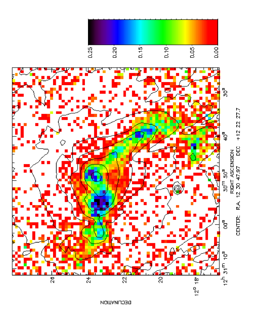
Figure 6: Emission integral ratio map, derived from EPIC data, overlaid on intensity contours, pixels are $10^{\prime\prime}\times 10^{\prime\prime}$ or 750pc$\times$750pc. The color palette on the right shows the correspondence between colors and Emission Integral ratios.

Our analysis shows that the volume occupied by the cooler phase is, for all regions, much smaller than the volume occupied by the hot phase. Moreover the size of the individual structures, possibly blobs, producing the cool emission, must be considerably smaller than the size of the regions for which we have accumulated spectra. To place tighter constraints on the size of these structures we have produced an emission integral ratio map according to the following procedure. We have produced two images: a “soft” image, S, extracting events from the 0.8-1.0 keV band, where the ratio of the cool component to the hot component is largest and a “hard” image, H, extracting events from the 0.5-0.7 keV and 1.1-4.0 keV bands where, on the contrary, the hot dominates over the cool emission. Assuming a cool component temperature of 0.85 keV and a hot component temperature of 1.7 keV, we have expressed the ratio of the soft component to the hot component in the soft band as a function of the counts in the soft and hard bands. We have then converted this in a cool over hot component emission integral ratio and reported the resulting map in Figure 6. As can be seen, the cool component emission is concentrated in the SW and E arms. Moreover the emission integral of the cool component is always between 0.01 and 0.2 of that of the hot component, roughly corresponding to a $V_{c}/V_{h}$ ratio in the range 0.0025 to 0.07 if we use eq. (1) and 0.005 to 0.14 if we correct for the factor of 2 found when comparing results obtained from eq. (1) to those obtained using deprojected values for $n_{h}$.

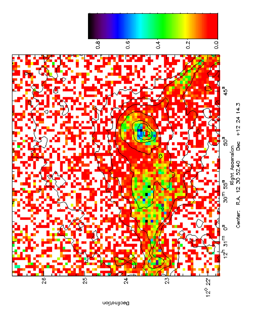
Figure 7: Emission integral ratio map, derived from Chandra data, overlaid on intensity contour, pixels are $4^{\prime\prime}\times 4^{\prime\prime}$ or 300pc$\times$300pc. The color palette on the right shows the correspondence between colors and Emission Integral ratios.

The obvious implication is that, even when pushing the resolution of the EPIC image to its limits and perhaps a little beyond (the pixels in our images are $10\arcmin\arcmin\times 10\arcmin\arcmin$ ) we still do not resolve the cool component blobs. To further constrain the size of the cool component structures we have produced a new emission integral ratio map using a Chandra observation of M87. The observation was carried out with the S3 chip in the aim point between the 29th and 30th of July 2000, the total effective exposure time, after minor cleaning for flares, is $\sim$35.3 ks, data was reprocessed using version 2.2.1 of CIAO and 2.10 of the calibration database. Thanks to the better spatial resolution of Chandra and high surface brightness of M87 we can employ $4\arcmin\arcmin\times 4\arcmin\arcmin$ pixels corresponding to 300 pc $\times$ 300 pc. The map has been produced following the same procedure adopted for the EPIC data. The Chandra map, see Figure 7, yields emission integral ratios similar to those found from the EPIC map, indicating that in most regions the size of the cool blobs is smaller than the resolution of the Chandra image. There is however one region 5$\times$2 pixels in size, localized $\sim 10\arcmin\arcmin$ N of the nucleus, where the ratio has an unusually high value of $\sim 0.7$. In this region we may be observing a cool component blob with a linear size of $\sim$ 1 kpc. Our assessments of the typical sizes of blobs are ofcourse rather crude, and are only meant as order of magnitude estimates. More detailed estimates would probably require comparisons with simulations in three dimensions.

The survival of small cool blobs embedded in a hotter medium brings us to the role of thermal conduction. In the absence of any inhibition, the timescale over which the blobs will evaporate from contact with the hotter gas is very short, assuming a typical size of 300 pc and density of $3\times 10^{-2}$ cm^-3, the conduction timescale is a few times $10^{5}$ yr (note that, even though we consider relatively small sizes, we do not expect conduction to be saturated as the mean free path for electrons is roughly ten times smaller). Thus, either blobs are continuously generated by an unknown mechanism or they survive thanks to substantial suppression of thermal conduction. It is hard to envisage a mechanism capable of continuously generating cool blobs for at least two reasons, firstly because the thermal conduction timescale is shorter than other timescales, such as the sonic or the cooling timescales on which such a mechanism may operate; secondly because, as we shall discuss in more detail later, the entropy of the cool blobs is smaller than that of the hotter gas from which they would presumably be formed. Thus the most likely scenario is one in which thermal conduction is suppressed. Assuming that the age of the blobs is equal or larger than the timescale over which the radio bubbles rise through the cluster atmosphere (a few times 10⁷ yr) we estimate that conduction must be suppressed by a factor of 100 or more. For many years it has been recognized that heat conduction might be suppressed in the ICM (e.g. Binney and Cowie 1981), and many authors (e.g. Chandran et al. 1999) have invoked magnetic fields as a possible means to achieve suppression. It is therefore quite remarkable that we find evidence of suppression only in those regions of M87 where we know magnetic field are present because we see radio halos.

In Figure 8 we show the entropy $S$, defined as $S\equiv T/n^{2/3}$, for the cooler and hotter components as a function of the radius. The density is estimated from a spectral deprojection of the data (Pizzolato et al. in prep.), while the temperature is the emission weighted temperature measured directly from spectral fits, using the density profile presented in Matsushita et al. (2002) produces very similar results. As can be seen, the entropy of the cool phase is virtually everywhere smaller than the entropy of the hot phase. This brings us to the rather important question of how the cool blobs where formed.

In a recent paper Churazov et al. (2001) have developed a detailed model to explain the radio and X-ray structure observed in M87. The authors envisage a scenario in which radio bubbles rise subsonically through the cluster atmosphere. As the bubbles rise, they capture ambient gas, dragging it upwards, during its upward motion the entrained gas is expected to evolve adiabatically. The above model was constructed to satisfy, amongst others, constraints coming from X-ray observations carried out with the ROSAT satellite. It is therefore important to test whether the model can live up to the better quality XMM-Newton EPIC and Chandra ACIS data. The model fails to explain two fundamental observational facts. Firstly, the model predicts that as the blobs rise their temperature drops adiabatically, while from Figure 5 we observe that the blob temperatures are remarkably contained everywhere between 0.8 and 1.0 keV, with no indication of a temperature drop with increasing radius. Secondly, since the cooler gas entropy is virtually everywhere smaller than the hotter gas entropy (see Fig. 8), the cooler gas cannot result from adiabatic expansion of the hotter gas entrained by the radio bubbles. Even assuming a conservative indetermination of a factor 2 on our relative entropy estimates we can allow for an adiabatic evolution only of those blobs currently located at radii larger than $\simeq 2^{\prime}$, blobs at smaller distances from the core would remain unexplained. Note also that, since the timescale on which the bubbles rise, a few times $10^{7}$ years, is smaller than the cooling timescale of the gas, a few times $10^{8}$ years, the entropy of the entrained gas cannot have been reduced through cooling.

The lack of a temperature gradient for the cool gas argues against a long adiabatic rise of the blobs through the cluster atmosphere. As suggested by Nulsen et al. (2001), the entrainment of the cool blobs from the radio bubbles may be unstable, thus the blobs could be captured and then released after having risen only a short way. If conduction is suppressed by magnetic fields associated to the bubble than the release of the blob from the bubble could be rapidly followed by heating of the blob to the ambient gas temperature, this could explain the clear separation between the cool and the hot gas temperatures.

Perhaps the most puzzling issue is the low entropy of the cool blobs. As already pointed out, this argues against the cool blobs originating from the ambient gas. One possible solution is to assume that, as envisaged by Fabian et al. (2001), metals are distributed in a highly inhomogeneous way in the ICM. If, for example, about 1% percent of the gas had a metallicity of 50, in solar units, and the rest of the gas had a metallicity of 1/2, again in solar units, than the metal rich gas would cool at a rate more than 20 times faster than the metal poor gas. Outside the region dominated by radio bubbles thermal conduction would maintain the metal rich blobs at the same temperature of the metal poor gas. In the radio bubbles, where magnetic fields suppress conduction, the metal rich gas would cool on timescales comparable or even shorter than those on which the radio bubbles rise through the cluster atmosphere. In this scenario the cool blobs are metal rich lumps which are kept at a roughly constant temperature due to a balance between radiative cooling and suppressed thermal conduction. Indeed, even if conduction is suppressed, cooling of the blobs increases the gradient between the cool and the hot phase making conduction more efficient. The entropy problem would also be solved because, as the metal rich lumps cool, they radiate away entropy. Unfortunately this rather attractive scenario does not do well when tested against the EPIC data. When fitting some of the spectra of the 2 temperature regions with a 2 temperature model allowing the Fe abundance of the two components to vary independently, we find that the Fe abundance of the cool component cannot be larger than 3-4 in solar units, even when using 99% confidence intervals.

Another alternative to explain the low entropy of the cool blobs is to assume that they have been generated by heating of cooler gas, perhaps through interaction with the radio lobes. However detailed studies at longer wavelengths have shown that the mass of cold gas present in M87 is orders of magnitudes smaller than the mass of the cool phase gas which we observe in X-rays. For instance Sparks et al. (1993) estimate a total mass of the order of $10^{5}-10^{7}M_{\odot}$ in the form of ionized gas in dusty filaments, while Edge (2001) derives an upper limit of $\sim 1.5\times 10^{8}M_{\odot}$ for any molecular gas, this is to be compared with a total mass of about $4\times 10^{9}M_{\odot}$ for the cool component, which we estimate from our measurements. A possible way out would be to assume that the gas has all been heated up, as might be expected if the core of M87 had recently undergone a starburst phase. If this were to be the case, we would expect to observe an enhancement in the abundance of heavy element. As discussed in Gastaldello and Molendi (2002) and in Canizares et al. (1982) we do indeed have evidence of an O overabundance in the core of M87, however a simple estimate of the mass of the starburst required to explain the O excess yields $4-5\times 10^{8}$ M_⊙, which is an order of magnitude smaller than the mass of the cool gas we observe at X-ray wavelengths.

5 Summary

We have performed an analysis of M87 using XMM-Newton EPIC and Chandra ACIS data. Our main findings may be summarized as follows.

• Spectra for most regions of M87 can be adequately fit by single temperature models. It is only for a few regions, which are cospatial with the E and SW radio arms, that we find evidence of a second temperature. Fitting more complicated spectral models to these regions (i.e. including a third temperature or a cooling-flow component) does not improve the quality of the fits.

• The lack of X-ray “holes” at the location of the SW and E radio arms indicates that the radio plasma has a small filling factor. As already suggested by Owen et al. (2000) the radio structures are most likely highly filamented with the interfilamentary regions dominated by the hot phase thermal plasma.

• The cool component fills a small volume compared to the hot component, it is probably structured in blobs with typical linear sizes smaller than a few 100 pc.

• Thermal conduction must be suppressed for these blobs to survive in the hotter ambient gas. Since the cool gas is observed only in those regions of M87 where we have evidence of radio halos our results provide important evidence that magnetic fields could be responsible for the suppression of heat conduction.

• The model proposed by Churazov et al. (2001) is found to be in contradiction with our observational results in two major aspects. Firstly, it predicts that as the blobs rise their temperature drops adiabatically, while we find no indication of a temperature drop with increasing radius. Secondly, the entropy of the cool blobs is in general smaller than that of the hot phase gas, thus cool blobs cannot originate from adiabatic evolution of hot phase gas entrained by buoyant radio bubbles, as suggested by Churazov et al. (2001).

• We have investigated two alternative solutions to solve the puzzle of the low entropy of the cool blobs. The first solution requires that the blobs, which originate from higher entropy ambient gas, rapidly radiate away their excess entropy thanks to their high metal content. However detailed spectral modeling of the EPIC data does not allow for a very high metal content of the cool blobs. The second assumes the cool gas originates from heating of cold gas. However, current estimates of the mass of cold gas are orders of magnitude smaller than the mass of cool gas we observe $\sim 4\times 10^{9}M_{\odot}$. Thus, at the present time, we are not capable of providing a convincing origin for the cool gas we observe in M87.

Figure 3: Ratio of the 90% confidence upper limit for the normalization of the third temperature component over the normalization of the cool component, as determined from the 2 temperature fit, versus the temperature of the third component. The spectrum used for this exercise is from the sector with bounding radii 2^′ and 3^′ and bounding angles 150^o and 180^o (angles are counted starting from West and going counter clockwise).

Figure 4: Normalized Emission Integral, i.e. EI/Area, versus radius. EI $\equiv{10^{-14}\over 4\pi d_{A}^{2}(1+z)^{2}}\int n_{e}n_{H}dV$, where $d_{A}$ is the angular distance to the source in cm, $z$ is the redshift, $n_{e}$ is the electron density in cm^-3, and $n_{H}$ is the hydrogen density in cm^-3. Area is in units of arcmin². Full circles are measurements from 1 temperature regions, empty circles and empty triangles indicate respectively measurements for the hot and cool components in 2 temperature regions.

Figure 5: Temperature versus radius. Symbols as in Fig. 4.

Figure 8: Entropy, defined as $S\equiv kT/n^{2/3}$, versus radius for 2 temperature regions. Full and empty circles indicate respectively measurements for the hot and cool component.

References

- (1) Arnaud, M., Neumann, D. M., Aghanim, N., Gastaud, R., Majerowicz, S., & Hughes, J. P. 2001, A&A, 365, L80
- (2) Belsole, E., Sauvageot, J. L., B hringer, H., Worrall, D. M.; Matsushita, K., Mushotzky, R. F., Sakelliou, I., Molendi, S., Ehle, M., Kennea, J., & Stewart, G. 2001, A&A, 365, L188
- (3) Binney, J., Cowie, L. L. 1981, ApJ, 247, 464
- (4) Bohringer, H., Nulsen, P.E.J., Braun, R., Fabian, A.C. 1995, MNRAS, 274, L67
- (5) Böhringer, H., Belsole, E., Kennea, J., Matsushita, K., Molendi, S., Worrall, D. M., Mushotzky, R. F., Ehle, M., Guainazzi, M., Sakelliou, I., Stewart, G., Vestrand, W. T., Dos Santos, S. 2001, A&A, 365, L181
- (6) Canizares, C. R., Clark, G. W., Jernigan, J. G.; Markert, T. H. 1982, ApJ, 262, 33
- (7) Chandran, B.D.G., Cowley, S.C., Albright, B 1999, in Proceedings of the Workshop held at Ringberg Castle, Germany, April 19-23, 1999., p.242
- (8) Churazov, E., Brüggen, M., Kaiser, C. R., Böhringer, H., Forman, W. 2001, ApJ, 554, 261
- (9) Edge, A.C 2001, MNRAS, 328, 762
- (10) Fabian, A.C., Mushotzky R.F., Nulsen P.E.J., & Peterson J.R. 2001, MNRAS, 321, L20
- (11) Gastaldello, F., Molendi, S. 2002, Apj in press
- (12) Ikebe, Y., Ezawa, H., Fukazawa, Y., Hirayama, M., Izhisaki, Y., Kikuchi, K., Kubo, H., Makishima, K., Matsushita, K., Ohashi, T., Takahashi, T., Tamura, T. 1996, Nature, 379, 427
- (13) Lieu, R., Mittaz, J. P. D., Bowyer, S., et al. 1996, ApJ, 458, L5
- (14) Makishima, K., Ezawa, H., Fukuzawa, Y., Honda, H., Ikebe, Y., Kamae, T., Kikuchi, K., Matsushita, K., Nakazawa, K., Ohashi, T., Takahashi, T., Tamura, T., Xu, H. 2001, PASJ, 53, 401
- (15) Molendi, S., Pizzolato, F. 2001, ApJ, 560, 194
- (16) Molendi, S., Gastaldello, F. 2001, A&A, 375, L14
- (17) Nulsen, P. E. J., David, L. P., McNamara, B. R., Jones, C., Forman, W. R., Wise, M. 2002, ApJ, 568,163
- (18) Owen, F. N., Eilek, J. A., Kassim, N. E. 2000, ApJ, 543, 611
- (19) Pizzolato et al. in prep.
- (20) Sparks, W. B., Ford, H. C., Kinney, A. L. 1993, ApJ, 413, 531
- (21) Young, A.J., Wilson, A.S., Mundell, C.G. 2002, submitted to ApJ