Differential rotation and meridional flow in the solar supergranulation layer: Measuring the eddy viscosity

We measure the eddy viscosity in the outermost layers of the solar convection zone by comparing the rotation law computed with the Reynolds stress resulting from f-plane simulations of the angular momentum transport in rotating convection with the observed differential rotation pattern. The simulations lead to a negative vertical and a positive horizontal angular momentum transport. The consequence is a subrotation of the outermost layers, as it is indeed indicated both by helioseismology and the observed rotation rates of sunspots. In order to reproduce the observed gradient of the rotation rate a value of about $1.5\times 10^{13}$ cm²/s for the eddy viscosity is necessary. Comparison with the magnetic eddy diffusivity derived from the sunspot decay yields a surprisingly large magnetic Prandtl number of 150 for the supergranulation layer. The negative gradient of the rotation rate also drives a surface meridional flow towards the poles, in agreement with the results from Doppler measurements. The successful reproduction of the abnormally positive horizontal cross correlation (on the northern hemisphere) observed for bipolar groups then provides an independent test for the resulting eddy viscosity.

1 Introduction and observations

Over the last years, while observing the solar oscillations on longer timescales and with higher precision, it has become evident that these oscillations play an important role in understanding the solar interior, bearing more or less the only information from the deeper parts of the sun, which cannot be probed otherwise. Helioseismology reveals a maximum of the angular velocity at all latitudes rather close to the surface, as shown in Fig. 1 (Howe et al. 2000).

It is known, on the other hand, that sunspots rotate faster than the solar surface plasma by about 4 % or 80 m/s at all latitudes. Such a clearly verified subrotation of the outermost layer of the convection zone is easiest understood as a result of angular momentum conservation of fluid elements with purely radial motions. But in this domain of the solar convection zone the velocity field is dominated by horizontal motions. Fluctuating fields with predominantly horizontal intensity should produce superrotation rather than subrotation. There is, however, another strong argument for considering the exceptional behavior of the horizontal motions in more detail.

Ward (1965) was the first to consider the horizontal cross-correlation of the proper motions of sunspot groups, the faster of which tend to move toward the equator. He found

$$Q_{\theta\phi}\approx\ 0.1\ ({\rm deg/day})^{2}\approx 2\times 10^{7}{\rm cm}^{2}/{\rm s}^{2}$$ (1)

on the northern hemisphere. More recent observations found smaller, but always positive values (Gilman & Howard 1984; Nesme-Ribes et al. 1993; Komm et al. 1994, see an overview by Meunier et al. 1997). This result has a strong implication for theory confirming the existence of the positive $H$ coefficient in the expression (3) for the horizontal Reynolds stress.

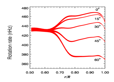
Figure 1: The internal rotation of the Sun as found by helioseismology. Image: NSF’s National Solar Observatory

We shall demonstrate the close relation between the negative radial gradient of the rotation rate and the positive sign of the horizontal cross correlation by solving the Reynolds equation on the basis of new data from hydrodynamic simulations of rotating convection in the outermost layer of the convection zone. The computations provide a tool for measuring the eddy viscosity in the outer solar convection zone.

2 The Reynolds stress

We start with the construction of the two components of the Reynolds stress tensor,

$$Q_{ij}=\langle u_{i}^{\prime}(\mbox{\boldmath$x$},t)u_{j}^{\prime}(\mbox{\boldmath$x$},t)\rangle,$$ (2)

which describe the angular momentum transport, i.e.

$$Q_{r\phi} = -\nu_{\rm T}r{\partial{\it\Omega}\over\partial r}\sin\theta+I\cdot V\sin\theta,$$

$$Q_{\theta\phi} = -\nu_{\rm T}{\partial{\it\Omega}\over\partial\theta}\sin\theta+I\cdot H\cos\theta.$$ (3)

Due to the terms containing the quantity $I$, angular momentum is transported even in case of rigid rotation, ${\it\Omega}=$ const.. This non-diffusive part of the stress, which only exists in case of anisotropic turbulence subject to a basic rotation, is known as the $\Lambda$-effect (Rüdiger 1989). The problem of the angular velocity gradient in the outer part of the solar convection zone has already been discussed by Gilman & Foukal (1979) and Gailitis & Rüdiger (1981) with theories based on the $\Lambda$-effect.

The stress (3) contains three unknown parameters, which determine the internal rotation law: the vertical angular momentum transport $V$, the horizontal angular momentum transport $H$, and the eddy viscosity $\nu_{\rm T}$. If the rotation law is known from observations and the $\Lambda$-effect is known from simulations, one should be able to measure the eddy viscosity. Once all three parameters are known we can compute a theoretical Ward profile, which can then be compared with the observed one as a test.

In (3), we have introduced the turbulence intensity,

$$I=\sqrt{\langle u_{r}^{\prime 2}\rangle\langle u_{\phi}^{\prime 2}\rangle},$$ (4)

from the simulations to normalize the $\Lambda$-effect. The functions $V$ and $H$ are also known from the simulations, but not the eddy viscosity, which we shall choose such that the observations are reproduced. With the same normalization for the eddy viscosity as for the $\Lambda$-effect, i.e.

$$\nu_{\rm T}=\tilde{\nu}\ {I\over{\it\Omega}},$$ (5)

the Reynolds stress reads

$$Q_{r\phi} = {I\over{\it\Omega}}\bigg{(}-\tilde{\nu}r{\partial{\it\Omega}\over\partial r}+V{\it\Omega}\bigg{)}\sin\theta,$$

$$Q_{\theta\phi} = {I\over{\it\Omega}}\bigg{(}-\tilde{\nu}{\partial{\it\Omega}\over\partial\theta}\sin\theta+H{\it\Omega}\cos\theta\bigg{)},$$ (6)

with $\tilde{\nu}$ as the only free parameter. It is varied between 0 and 1 in order to reproduce the observed value of 5% for the decrease of the rotation rate with radius. It is obvious that large values of $\tilde{\nu}$ will produce negative (positive) cross correlations on the northern (southern) hemisphere, while small numbers of $\tilde{\nu}$ and positive values of $H$ are required for the observed (opposite) behavior. Indeed, as we have scaled the eddy viscosity with the rotation period rather than with the convective turnover time in (5), we must expect a rather small value for $\tilde{\nu}$. As the eddy viscosity in the solar convection zone fixes the value of the Taylor number, the Taylor number fixes the amplitude of the meridional flow, and the meridional flow might fix the solar dynamo, it is important to derive the eddy viscosity from observations.

3 The simulations

We obtain the functions $V$ and $H$ from the f-plane numerical simulations of Chan (2001). These calculations computed rotating convection in local pieces of the spherical shell and obtained values of the turbulence Reynolds stress at a different latitudes. The latitudinal coverage of the cases is dense enough for us to obtain analytical fits of the numerical data. The strong density stratification is completely included in the model simulations, as is the energy transport by radiation (gradient of temperature) and convection (gradient of entropy).

The resulting $\Lambda$-effect from the ${\it\Omega}=1/2,F/0.25=1/8$ case, as tabulated in Chan (2001, Table 3), is given in the Figs. 2 and 3 showing the data from the simulation vs. the expansions of Eqs. (8) and (9). The main feature of the vertical $\Lambda$-effect, $V$, is its negative sign (see Fig. 2) while the horizontal $\Lambda$-effect, $H$, proves to be positive (see Fig. 3).

After the theory of the $\Lambda$-effect, the vertical transport can be approximated with $V\propto\langle u_{\phi}^{\prime 2}\rangle-\langle u_{r}^{\prime 2}\rangle$ for slow rotation, so that predominantly vertical turbulence, $\langle u_{r}^{\prime 2}\rangle>\langle u_{\phi}^{\prime 2}\rangle$, is needed for $V$ to assume negative values. As Table 2 in Chan (2001) shows, this is indeed the case.

Figure 2: The latitudinal profile of the vertical $\Lambda$-effect, $V$. Solid line: values from Chan (2001), dash-dotted line: The profile described by Eq. (8)

Figure 3: The latitudinal profile of the horizontal $\Lambda$-effect, $H$. Solid line: values from Chan (2001), dash-dotted line: The profile described by Eq. (9)

By the signs of both $H$ and $V$, these results are very promising in order to reproduce the negative slope of the rotation rate as well as the positive sign of the horizontal cross correlations. However, in contrast to expectations, $V$ exhibits a minimum at the equator while $H$ is highly concentrated at low latitudes.

As in Rüdiger (1989), the $\Lambda$-effect terms in (8) and (9) are written as

$$V=\sum_{l=0}V^{(l)}\sin^{2l}\theta,\quad H=\sum_{l=1}H^{(l)}\sin^{2l}\theta,$$ (7)

so that the result of the simulations can be summarized with the series expansion

$$V = -0.300+0.187\sin^{2}\theta+0.0158\sin^{4}\theta+$$ (8)

$$\qquad\qquad\qquad+0.0337\sin^{6}\theta,$$

and

$$H=0.727\sin^{6}\theta,$$ (9)

so that

$$V^{(0)} = -0.30,\qquad\qquad\qquad\ \ V^{(1)}=0.19,$$

$$V^{(2)} = \ \ \ 0.016,\qquad\qquad\qquad V^{(3)}=0.034,$$ (10)

$$H^{(1)} = H^{(2)}=0,\qquad\qquad\ \ \ \ \ H^{(3)}=0.73$$

results. These results are very interesting insofar as the surface effects of the convection zone are included in the model, in contrast to the computation of the $\Lambda$-effect for free turbulence by Kitchatinov & Rüdiger (1993, KR93). In the latter model the $\Lambda$-effect is a function of the Coriolis number,

$$\Omega^{*}=4\pi\frac{\tau_{\rm corr}}{P_{\rm rot}},$$ (11)

where $\tau_{\rm corr}$ is the convective turnover time and $P_{\rm rot}$ the rotation period. The result is shown in Fig. 4. For slow rotation, $\Omega^{*}\ll 1$, positive values result for $V^{(0)}$, and $V^{(1)}=H^{(1)}$ is small but negative. On the other hand, for fast rotation one finds $V^{(0)}<0$ and $V^{(1)}=H^{(1)}\lower 1.72218pt\hbox{$\;\buildrel>\over{\scriptstyle\sim}\;$}0$ similar to the numbers in Figs. 2 and 3. In the supergranulation layer of the solar convection zone, however, one cannot apply the results for $\Omega^{*}\gg 1$.

The values in (10) differ considerably from the predictions of the KR93 theory indicating that the latter is invalid for the outermost layers of the convection zone, where surface effects such as the presence of a boundary, strong density stratification, and radiation transport are essential.

Figure 4: The turbulence-originated coefficients in the non-diffusive fluxes of angular momentum in the solar convection zone from KR93. Solid line: $V^{(0)}$. Dashed line: $V^{(1)}=\mbox{\boldmath$H$}^{(1)}$. Note that $V^{(0)}$ is positive for slow rotation

4 The solution

We are looking for the eddy viscosity parameter $\tilde{\nu}$. It must be positive and it must reproduce the 5% radial decrease of the rotation rate through the supergranulation layer. With the expressions (6), we solve the Reynolds equation,

$$\rho\left[\frac{\partial\mbox{\boldmath$\bar{u}$}}{\partial t}+(\mbox{\boldmath$\bar{u}$}\cdot\nabla)\mbox{\boldmath$\bar{u}$}\right]=-\nabla p-\nabla\cdot(\rho Q)+\rho\mbox{\boldmath$g$},$$ (12)

assuming axisymmetry and under the anelastic approximation,

$$\nabla\cdot(\rho\mbox{\boldmath$\bar{u}$})=0.$$ (13)

In cases where the meridional flow can be neglected, the azimuthal component of Eq. (12) is reduced to

$$\nabla\cdot(r\sin\theta\rho\langle u^{\prime}_{\phi}\mbox{\boldmath$u^{\prime}$}\rangle)=0.$$ (14)

Expanding the rotation rate in terms of Legendre functions,

$${\it\Omega}={\it\Omega}_{0}\sum\omega_{n-1}(x){P_{n}^{(1)}(\cos\theta)\over\sin\theta},$$ (15)

Eq. (14) can be solved analytically for a thin layer with stress-free boundary conditions,

$$Q_{r\phi}=0,$$ (16)

as described in detail by Rüdiger (1989). The boundary conditions,

$$\tilde{\nu}\omega_{0}^{\prime}=V_{0}\quad\tilde{\nu}\omega_{2}^{\prime}=V_{2},$$ (17)

where $V_{n}$ now are the components of the function $V$ expanded in terms of orthogonal polynomials, lead to

$$V_{0} = V^{(0)}+0.8V^{(1)}+0.069V^{(2)}\simeq-0.15,$$

$$V_{1} \simeq -0.02.$$ (18)

Inserting the slope $\omega_{0}^{\prime}\simeq-1.4$ from the observed rotation law in Eqs. (17) and (18), we obtain

$$\tilde{\nu}\simeq 0.11$$ (19)

for the eddy viscosity.

The derivation of the result (19) is only valid for a very thin surface layer. To treat a layer of finite depth, we solve Eq. (12) numerically with $\tilde{\nu}$ as an input parameter. At the lower boundary, at $x_{\rm in}$=0.95, we prescribe the rotation law,

$${\it\Omega}(\theta)={\it\Omega}_{0}(0.7+0.3\sin^{2}\theta),$$ (20)

to impose the observed latitudinal shear. The upper boundary is stress-free. The density stratification is taken from a standard solar model (Ahrens et al. 1992). The code used is the same as in Küker & Stix (2001). We have made runs with and without the meridional flow included and found no significant difference between the results. The results shown in Fig. 5 were obtained with the meridional flow included.

Indeed a negative slope of the rotation law results for all latitudes. Its amplitude grows with decreasing viscosity. For

$$\tilde{\nu}=0.1$$ (21)

the results in the Fig. 5 comply with the observations. Again the $\partial{\it\Omega}/\partial r$ is negative for all latitudes.

Figure 5: Rotation rate at the equator, 15, 30, 45, and 60 degrees latitude (from top to bottom) in the outermost region of the solar convection zone for $\tilde{\nu}=0.3$ (left), $\tilde{\nu}=0.1$ (middle), $\tilde{\nu}=0.03$ (right)

5 Eddy viscosity and magnetic Prandtl number

As there are no observations about (say) the decay of large-scale vortices at the solar surface, we have no direct information about the amplitude of the eddy viscosity. The only way to determine it is the study of the internal differential rotation of the Sun. We have shown that for $\tilde{\nu}\simeq$ 0.1 the observed radial gradients of the outer solar rotation law can be reproduced. It might be interesting to use this value to estimate the eddy viscosity amplitude in the outermost layers of the solar convection zone. With a RMS value of about 200 m/s for the velocity fluctuations (see Fig. 6),

$$\nu_{\rm T}\simeq 1.5\times 10^{13}\ \ {\rm cm^{2}/s}$$ (22)

follows from Eq. (5).

Figure 6: The turbulence intensity in the solar supergranulation layer after Ahrens et al. (1992)

In stellar magnetohydrodynamics, the turbulent magnetic Prandtl number, Pm=$\nu_{\rm T}$/$\eta_{\rm T}$, is an important parameter. It is often assumed to be of order unity, but this is not finally clear. The advection-dominated solar dynamo, e.g., requires an eddy magnetic diffusivity smaller than $10^{12}$ cm²/s (Choudhuri et al. 1995, Dikpati & Charbonneau 1999, Küker et al. 2001), hence after (22) a turbulent magnetic Prandtl number greater than 15. The value increases to Pm $\simeq 150$ if – as it is suggestive – the eddy magnetic diffusivity, $\eta_{\rm T}$, is derived from the sunspot decay ($\simeq 10^{11}$cm²/s). The dispersal of large-scale patterns in the surface magnetic flux, however indicates a considerably larger value of $6\times 10^{12}$ cm²/s for the eddy magnetic diffusivity (Sheeley 1992), hence a turbulent magnetic Prandtl number of about 2.5.

Large values of the magnetic Prandtl number are not quite unreasonable. It is shown in Rüdiger (1989) that the turbulent Prandtl number runs with the inverse microscopic Prandtl number, which takes the value of 0.01 for the solar plasma and thus would indeed lead to values of about 100 for the turbulent magnetic Prandtl number.

6 The Ward profile

An important test is whether such viscosity values would generate the positive Ward profile. This is indeed the case. At low northern latitudes the horizontal cross correlation is positive, but we do not have any information about the higher latitudes. From the stress (6), we find for the Ward profile,

$$W=-{\tilde{\nu}\over{\it\Omega}}{\partial{\it\Omega}\over\partial\theta}\sin\theta+H\cos\theta.$$ (23)

The results for various values of $\tilde{\nu}$ are shown in Fig. 7. Note that the covariance is indeed positive (in the northern hemisphere) at low latitudes, and slightly negative at high latitudes, from where we do not have any reliable data.

Figure 7: The Ward profile W for $\tilde{\nu}=0.3,0.1,0.03$ (from top to bottom). The correlation is slightly negative in the high northern latitudes but it is positive as observed in low northern latitudes

7 The meridional flow

Doppler measurements find a surface meridional flow that is directed polewards with maximum speeds between 10 and 15 m/s (Komm et al. 1993). Models of solar differential rotation based on the KR93 Reynolds stress usually fail to produce this surface flow, though a corresponding flow cell exists in the bulk of the convection zone. It is, however, superseeded by a second flow cell in the surface layers with opposite flow direction, hence producing a surface flow towards the equator. This superficial flow cell is driven by the positive radial gradient of the rotation rate, which is due to the short convective turnover time (and thus small Coriolis number) in the supergranulation layer. Since the meridional flow is mainly driven by the gradient of the rotation rate in $z$-direction, the effect on the flow pattern is profound. With the $\Lambda$-effect from the Chan (2001) simulations, both the positive rotational shear and the additional flow cell vanish. Figure 8 shows the maximum surface flow speed as a function of the viscosity parameter $\tilde{\nu}$. Contrary to Kitchatinov & Rüdiger (1999) and Küker & Stix (2001), the surface flow is directed towards the poles, and (again) for the $\tilde{\nu}=0.1$ case (which best reproduces the radial shear) the flow speed lies in the observed range.

Figure 8: The amplitude of the poleward directed meridional flow at the solar surface

8 Conclusions

The theory of turbulent angular momentum transport in stellar convection zones based on the Second Order Correlation Approximation (SOCA) in KR93 predicts a positive vertical and vanishing horizontal $\Lambda$-effect in the solar supergranulation layer, and negative vertical as well as positive horizontal $\Lambda$-effect in the bulk of the solar convection zone. Solutions of the Reynolds equation with the stress tensor from KR93 therefore reproduce the observed variation of the rotation rate with latitude remarkably well, but lack the decrease of the rotation rate with increasing radius in the outermost part of the convection zone.

Simulations of rotating convection in the upper part of the solar convection zone show a strong and positive horizontal and a negative vertical $\Lambda$-effect. With the $\Lambda$-coefficients as derived from the simulations, the solutions show a negative shear, $\partial\Omega/\partial r<0$, of the observed amplitude when a value of $1.5\times 10^{13}{\rm cm}^{2}/{\rm s}$ is chosen for the eddy viscosity. As there is no way to directly measure the eddy viscosity, this is the only method to derive its value from observations.

As an independent test, we have computed theoretical Ward profiles. With the $\Lambda$-effect from KR93, the horizontal cross-correlation is always negative because the horizontal $\Lambda$-effect vanishes in the surface layer. With the large positive value of $H$ from the simulations, on the other hand, $Q_{\theta\phi}$ is always positive at low latitudes, as observed, and the amplitudes are in good agreement as well.

In models of the solar differential rotation with positive radial $\Lambda$-effect in the outermost layers of the convection zone, the radial shear is always positive in that layer, and the surface gas flow is directed towards the equator, both in contradiction to the observations. The negative radial $\Lambda$-effect derived from the Chan (2001) simulations removes both these contradictions by maintaining a negative gradient of the rotation rate, which in turn drives the surface flow towards the poles.

We conclude that the KR93 expressions for the Reynolds stress are invalid in the outermost part of the solar convection zone. Possible reasons are the proximinty of the outer boundary, the increasing importance of radiative energy transport with decreasing depth, and the neglect of the inherent anisotropy of turbulent convection, which is driven by a large-scale entropy gradient rather than a random force.

References

- (1) Ahrens, B., Stix, M., & Thorn, M. 1992, A&A, 264, 673
- (2) Chan, K.L. 2001, ApJ, 548, 1102
- (3) Choudhuri, A., Schüssler, M., Dikpati, M. 1995, A&A, 303, L29
- (4) Dikpati, M., & Charbonneau, P. 1999, ApJ, 518, 508
- (5) Gailitis, A., & Rüdiger, G. 1981, ApJ, L22, 89
- (6) Gilman, P.A., & Foukal, P.V. 1979, ApJ, 229, 1179
- (7) Gilman, P.A., & Howard, R.F. 1984, Solar Phys., 93, 171
- (8) Howe, R., Christensen-Dalsgaard, J., Hill, F., et al. 2000, Sci, 287, 2456
- (9) Kitchatinov, L. L., & Rüdiger, G. 1993, A&A, 276, 96, KR93
- (10) Kitchatinov, L. L., & Rüdiger, G. 1999, A&A, 344, 911
- (11) Komm, R.W., Howard, R.F., & Harvey, J.W. 1993, Solar Phys., 147, 207
- (12) Komm, R.W., Howard, R.F., & Harvey, J.W. 1994, Solar Phys., 151, 15
- (13) Küker, M., & Stix, M. 2001, A&A, 366, 668
- (14) Küker, M., Rüdiger, G., Schultz, M. 2001, A&A, 374, 301
- (15) Meunier, N., Proctor, M. R. E., Sokoloff, D. D., Soward, A. M., Tobias, S. M. 1997, GAFD, 86, 249
- (16) Nesme-Ribes, E., Ferreira, E.N., & Vince, L. 1993, A&A, 276, 211
- (17) Rüdiger, G. 1989, Differential Rotation and Stellar Convection: Sun and Solar-type Stars (Gordon & Breach Science Publishers, New York)
- (18) Sheeley, N.R. 1992, in K.L. Harvey (ed.), The Solar Cycle, A.S.P. Conf. Series Vol. 27, Astron. Soc. of the Pac., San Francisco
- (19) Ward, F. 1965, ApJ, 141, 534