Gabor Transforms on the Sphere with Applications to CMB Power Spectrum Estimation

Abstract

The Fourier transform of a dataset apodised with a window function is known as the Gabor transform. In this paper we extend the Gabor transform formalism to the sphere with the intention of applying it to CMB data analysis. The Gabor coefficients on the sphere known as the pseudo power spectrum is studied for windows of different size. By assuming that the pseudo power spectrum coefficients are Gaussian distributed, we formulate a likelihood ansatz using these as input parameters to estimate the full sky power spectrum from a patch on the sky. Since this likelihood can be calculated quickly without having to invert huge matrices, this allows for fast power spectrum estimation. By using the pseudo power spectrum from several patches on the sky together, the full sky power spectrum can be estimated from full-sky or nearly full-sky observations.

1 introduction

The Cosmic Microwave Background (CMB) is one of our most important sources of information about the early universe [Bond 1995, Jungman et al. 1996, Hu, Sugiyama & Silk 1997, Durrer 2001]. The pattern of the temperature fluctuations in the CMB contains information about a number of cosmological parameters. If the temperature fluctuations are Gaussian as predicted by most models of the early universe, all this information is stored in the angular power spectrum coefficients $C_{\ell}$. For this reason, several experiments have been conducted to measure the CMB power spectrum. The COBE satellite discovered the fluctuations in 1992 [G. F. Smoot et al. 1992], and since then several ground based and balloon borne experiments [De Bernardis et al. 2000, Hanany et al. 2000, Netterfield et al. 2001, Lee et al. 2001, Halverson et al. 2001, Pryke et al. 2001] have been made to study the CMB at an ever increasing resolution. As the amount of CMB data from these experiments is rapidly growing, the task of extracting the power spectrum from the data is getting harder.

Analysing the CMB data from a given experiment consists of several steps as the data consists of several components not belonging to the CMB [Maino et al. 2001, Stolyarov et al. 2001]. In this paper, we will concentrate on extracting the power spectrum from a CMB map with foregrounds removed. The standard method of extracting the power spectrum from a sky map is the method of maximum likelihood. This method gives the smallest error bars on the power spectrum estimates, but has the drawback that the number of operations needed to perform the estimation, scales as $N_{\mathrm{pix}}^{3}$, where $N_{\mathrm{pix}}$ is the number of pixels in the map. For experiments with high resolution the number of pixels can be up to several million and this method becomes infeasible using current computers [Borrill 1999].

In [Oh, Spergel & Hinshaw 1999], it is shown how the likelihood analysis can be speeded up to scale as $N_{\mathrm{pix}}^{2}$ with assumptions about azimuthal symmetry and uncorrelated noise. Another $N_{\mathrm{pix}}^{3/2}$ method for large azimuthally symmetric parts of the sky with uncorrelated noise was presented in [Wandelt, Górski & Hivon 2000]. The likelihood problem can also be solved exact in $~{}N_{\mathrm{pix}}^{2}$ operations with correlated noise for special scanning strategies as demonstrated in [Wandelt 2000, Wandelt & Hansen 2001]. In [Bond 1995, Bond, Jaffe & Knox 2000, Bartlett et al. 2000] it is shown how one can approximate the likelihood to speed up the calculations, but still an $~{}N_{\mathrm{pix}}^{3}$ operation is needed. This has led people to find other estimators than the maximum likelihood estimator to extract the power spectrum. In [Tegmark, Taylor & Heavens 1997] an optimal estimator was found but the calculation scales as $N_{\mathrm{pix}}^{2}$ times a huge prefactor. Recently some near optimal estimators have been found which can be calculated in $~{}N_{\mathrm{pix}}^{2}$ operations [Dore, Knox & Peel 2001, Szapudi et al. 2000, Hivon et al. 2002] The data from the BOOMERANG [De Bernardis et al. 2000, Netterfield et al. 2001] experiment was analysed using the MASTER method [Hivon et al. 2002]. In this method, the power spectrum was extracted by a quadratic estimator based on the pseudo power spectrum (the power spectrum on the cut sky). A similar method was suggested by [Balbi et al. 2002] for the Planck surveyor. Here we propose to use the pseudo power spectrum ($\tilde{C}_{\ell}$) for likelihood estimation. This principle was also used in [Wandelt, Górski & Hivon 2000] but then for large sky coverage so that the correlations between the $\tilde{C}_{\ell}$ coefficients could be neglected.

In this paper, we study the effect of Gabor transforms on the sphere. Gabor transforms, or windowed Fourier transforms are just Fourier transforms where the function $f(x)$ to be Fourier transformed is multiplied with a Gabor window $W(x)$ [Gabor 1946]. In the discrete case $f(x_{i})$ can be a data stream. If parts of the data stream are of poor quality or is missing, this can be represented as $W(x_{i})f(x_{i})$ where the window $W$ is zero where there are missing parts. The window can also be formed so that it smoothes the edges close to the missing parts and in this way avoid ringing in the Fourier spectrum.

We will study the effect of Gabor transforms on the sphere and use it for fast CMB power spectrum estimation. The Gabor transform in this context is just the multiplication of the CMB sky with a window function before using the spherical harmonic transform to get the Gabor transform coefficients in this case called the pseudo power spectrum. The window can be a top-hat to take out certain parts of the sky in the case of limited sky coverage. Another window can be a Gaussian Gabor window for smoothing the transition between the observed and unobserved area of the sky. The Gabor window can also be designed in such a way as to increase signal-to-noise by giving pixels with high signal-to-noise higher significance in the analysis. The use of the windowed Fourier transform was already studied in [Hobson & Magueijo 1996] in the flat-sky approximation. We show that some of their results are also valid on the sphere.

In the standard likelihood approach of power spectrum estimation, the pixels on the CMB sky or the spherical harmonic coefficients $a_{\ell m}$ are used as elements in the data vector in which case the correlation matrix will have dimensions of the order $N_{\mathrm{pix}}\times N_{\mathrm{pix}}$. A matrix of this size can not be inverted in a reasonable amount of time with current computers. We propose to use the pseudo power spectrum coefficients $\tilde{C}_{\ell}$ as elements of the data vector in the likelihood. In this case the size of the correlation matrix will at most be $l_{\mathrm{max}}\times l_{\mathrm{max}}$ which can be inverted in a few seconds. The most time consuming part is the calculation of the elements of the correlation matrix of pseudo-$C_{\ell}$.

In Section (2) we will first describe the one dimensional Gabor transform and then define the Gabor transform on the sphere. We will define the pseudo power spectrum which is just the Gabor coefficients on the CMB sky. The kernel relating the full sky power spectrum and the pseudo power spectrum for a Gaussian and top-hat Gabor window will be discussed. Then in Section (3) we will use the pseudo power spectrum as input values to a maximum likelihood estimation of the full sky power spectrum. The probability distribution of the pseudo power spectrum coefficients will be assumed Gaussian and we will show that this is a good approximation at high multipoles ($\ell>100$). Some examples of likelihood estimations of the power spectrum with different noise patterns will be shown. In Section (4) two extensions of the method will be discussed. First the use of the pseudo power spectrum from different Gabor windows centred at different points on the sphere simultaneously is demonstrated. In this way full-sky or nearly full-sky observations can be analysed. The second extension of the method is the use of Monte Carlo simulations to obtain noise properties in the case where this is faster than using the analytic expression or where the noise is correlated. Finally in Section (5) the results and further extensions are discussed.

2 The Gabor Transformation and the Temperature Power Spectrum

In this section we will first describe the Gabor transform for functions on a one dimensional line. Then we extend the formalism to functions on the sphere and the properties of the Gabor transform coefficients on the CMB sky, the pseudo-$C_{\ell}$, are discussed. As most CMB experiment will not be able to observe the full sky, it is important to study the properties of the power spectrum on the sky apodised with a window function. As we will show later, the best way to construct the window is not always to set it to $1$ in the observed area and to $0$ in the non-observed area of the sky. For this reason we will study the Gabor transform for windows with different profiles. On the cut sky the pseudo power spectrum coefficients will get coupled [Wandelt, Górski & Hivon 2000, Hivon et al. 2002]. We will study how strong this coupling is for different window sizes and for different windows. We will in particular study the top-hat and the Gaussian windows. The top-hat window is important, as it is the window which preserves most of the information in the observed data set. The Gaussian window smoothes of the edges between the observed and unobserved areas of the sky and in this way cuts off long range correlations between pseudo $C_{\ell}$.

2.1 The one dimensional Gabor transform

For a data set $d_{j}$ with N elements, the normal Fourier transform is defined as,

$$\tilde{d}_{k}=\sum_{j}d_{j}\mathrm{e}^{\mathrm{i}2\pi jk/N}.$$ (1)

A tilde on $\tilde{d}$ shows that these are the Fourier coefficients. The inverse transform is then,

$$d_{j}=\frac{1}{N}\sum_{k}\tilde{d}_{k}\mathrm{e}^{-\mathrm{i}2\pi jk/N}.$$ (2)

Sometimes it is useful to study the spectrum of just a part of the data set. This could be if some parts are of poor quality or the spectrum is changing along the data set. In this case, one can multiply the data set with a function, removing the unwanted parts and taking out a segment to be studied. The function can be a step function cutting out the segment to study with sharp edges or a function which smoothes the edges of the segment to avoid ringing (typically a Gaussian).

The Fourier transform with such a multiplication was studied by Gabor [Gabor 1946] and is called the Gabor Transform. It is defined for a segment centred at $j=M$ and with wavenumber $k$ as,

$$\tilde{d}_{kM}=\sum_{j}d_{j}G_{j-M}\mathrm{e}^{\mathrm{i}2\pi jk/N}.$$ (3)

Here $G_{j-M}$ is the Gabor window, the function to multiply the data set with. The transform is similar to the Wavelet transform. The difference is that the window function in the Wavelet transform is frequency dependent so that the size of the segment is changing with frequency.

Analogously to the Fourier transform, there is also an inverse Gabor transform. To recover the whole data set from a Gabor transform, one needs the Fourier coefficients taken with several windows $G_{j-M}$ being centred at different points $M$. This means that the data set has to be split into several segments. The centre of each segment is set to $M=mK$ where $K$ determines the density of segments and $m$ is an integer specifying the segment number. One then has for the inverse transform

$$d_{j}=\sum_{m}\sum_{k}\tilde{d}_{km}g_{km}.$$ (4)

Due to the non-orthogonality of the Gabor transform, the dual Gabor window $g_{km}$ is not trivial to find, but several techniques have been developed for calculating this dual window (e.g. [Strohmer 1997] and references therein).

In this paper we will study the Gabor transform on the sphere and apply it to CMB analysis. We will take out a disc on the CMB sky, using either top-hat or Gaussian apodisation and then derive the pseudo power spectrum $\tilde{C}_{\ell}$ on the apodised sky. The $\tilde{C}_{\ell}$ will be used for likelihood estimation of the underlying full sky power spectrum. We also show how several discs (segments) centred at different points can be combined to yield the full sky power spectrum.

2.2 Gabor transform on the sphere

We start by defining the $\tilde{C}_{\ell}$ for a Gabor window $G({\mathbf{\hat{n}}})$ as,

$$\tilde{C}_{\ell}=\sum_{m}\frac{\tilde{a}_{\ell m}^{*}\tilde{a}_{\ell m}}{2\ell+1},$$ (5)

where

$$\tilde{a}_{\ell m}=\int d{\mathbf{\hat{n}}}T({\mathbf{\hat{n}}})G({\mathbf{\hat{n}}})Y^{*}_{\ell m}({\mathbf{\hat{n}}}).$$ (6)

Here $T({\mathbf{\hat{n}}})$ is the observed temperature in the direction of the unit vector ${\mathbf{\hat{n}}}$, $Y_{\ell m}({\mathbf{\hat{n}}})$ is the spherical Harmonic function and $G({\mathbf{\hat{n}}})$ is the Gabor window. We now find an expression for the expectation value of $\tilde{C}_{\ell}$.

We will here use a Gabor window which is azimuthally symmetric about a point ${\mathbf{\hat{n}}}_{0}$ on the sphere, so that the window is only a function of the angular distance from this point on the sphere $\cos\theta={\mathbf{\hat{n}}}\cdot{\mathbf{\hat{n}}}_{0}$. Then one can write the Legendre expansion of the window as,

$$G(\theta)=\sum_{\ell}\frac{2\ell+1}{4\pi}g_{\ell}P_{\ell}(\cos\theta)=\sum_{\ell m}g_{\ell}Y_{\ell m}({\mathbf{\hat{n}}})Y^{*}_{\ell m}({\mathbf{\hat{n}}}_{0}).$$ (7)

One can also write,

$$T({\mathbf{\hat{n}}})=\sum_{\ell m}a_{\ell m}Y_{\ell m}({\mathbf{\hat{n}}}).$$ (8)

Inserting these two expressions in equation (6) one gets

$$\tilde{a}_{\ell m} = \sum_{\ell^{\prime}m^{\prime}}a_{\ell^{\prime}m^{\prime}}\sum_{\ell^{\prime\prime}m^{\prime\prime}}g_{\ell^{\prime\prime}}Y^{*}_{\ell^{\prime\prime}m^{\prime\prime}}({\mathbf{n}}_{0})\int Y^{*}_{\ell m}({\mathbf{\hat{n}}})Y_{\ell^{\prime}m^{\prime}}({\mathbf{\hat{n}}})Y_{\ell^{\prime\prime}m^{\prime\prime}}({\mathbf{\hat{n}}})d{\mathbf{\hat{n}}}$$ (9)

$$= \sum_{\ell^{\prime}m^{\prime}}a_{\ell^{\prime}m^{\prime}}\sum_{\ell^{\prime\prime}m^{\prime\prime}}g_{\ell^{\prime\prime}}Y^{*}_{\ell^{\prime\prime}m^{\prime\prime}}({\mathbf{\hat{n}}}_{0})\sqrt{\frac{(2\ell+1)(2\ell^{\prime}+1)(2\ell^{\prime\prime}+1)}{4\pi}}$$ (15)

$$\times{\left(\begin{array}[]{ccc}\ell&\ell^{\prime}&\ell^{\prime\prime}\\ -m&m^{\prime}&m^{\prime\prime}\\ \end{array}\right)}{\left(\begin{array}[]{ccc}\ell&\ell^{\prime}&\ell^{\prime\prime}\\ 0&0&0\\ \end{array}\right)}(-1)^{m},$$

where relation (43) for Wigner 3j Symbols were used. Using this expression, the relation $\langle a_{\ell m}^{*}a_{\ell^{\prime}m^{\prime}}\rangle=C_{\ell}\delta_{\ell\ell^{\prime}}\delta_{mm^{\prime}}$ and the orthogonality of Wigner symbols (equation 41), one can write $\langle\tilde{C}_{\ell}\rangle$ as,

$$\langle\tilde{C}_{\ell}\rangle=\sum_{\ell^{\prime}}C_{\ell^{\prime}}K(\ell,\ell^{\prime}).$$ (16)

With $C_{\ell}$ we will always mean $\langle C_{\ell}\rangle$ when we are referring to the full sky power spectrum. In this expression, $K(\ell,\ell^{\prime})$ is the Gabor kernel,

$$K(\ell,\ell^{\prime})=(2\ell^{\prime}+1)\sum_{\ell^{\prime\prime}}g_{\ell^{\prime\prime}}^{2}\frac{(2\ell^{\prime\prime}+1)}{(4\pi)^{2}}{\left(\begin{array}[]{ccc}\ell&\ell^{\prime}&\ell^{\prime\prime}\\ 0&0&0\\ \end{array}\right)}^{2}.$$ (17)

The Legendre coefficients $g_{\ell}$, are found by the inverse Legendre transformation,

$$g_{\ell}=2\pi\int_{\theta=0}^{\theta=\theta_{\mathrm{C}}}G(\theta)P_{\ell}(\cos\theta)d\cos\theta,$$ (18)

where $\theta_{\mathrm{C}}$ is the cut-off angle where the window goes to zero. One sees from the expression for the kernel, that there is no dependency on ${\mathbf{\hat{n}}}_{0}$. This means that $\langle\tilde{C}_{\ell}\rangle$ is the same, independent on where the Gabor window is centred. In the rest of this section we will study the shape of this kernel which couples the $\tilde{C}_{\ell}$ on the apodised sphere.

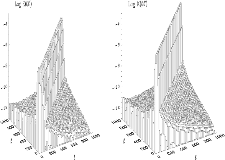
Figure 1: The logarithm of the kernel $K(\ell,\ell^{\prime})$ describing the connection between the spherical harmonic coefficients $C_{\ell}$ on the full sky and the corresponding coefficients $\tilde{C}_{\ell}$ on the apodised sky via the relation $\tilde{C}_{\ell}=\sum_{\ell^{\prime}}K(\ell,\ell^{\prime})C_{\ell^{\prime}}$. The figure shows the kernel for a $5^{\circ}$ and $15^{\circ}$ FWHM Gaussian Gabor window with $\theta_{\mathrm{C}}=3\sigma$ (left and right respectively).

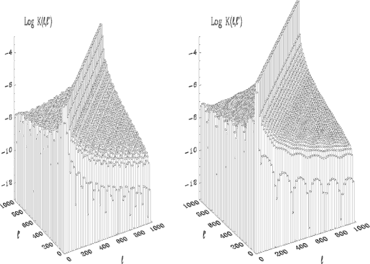
Figure 2: Same as Fig. 1 for top-hat Gabor windows covering the same area on the sky as the Gaussian windows.

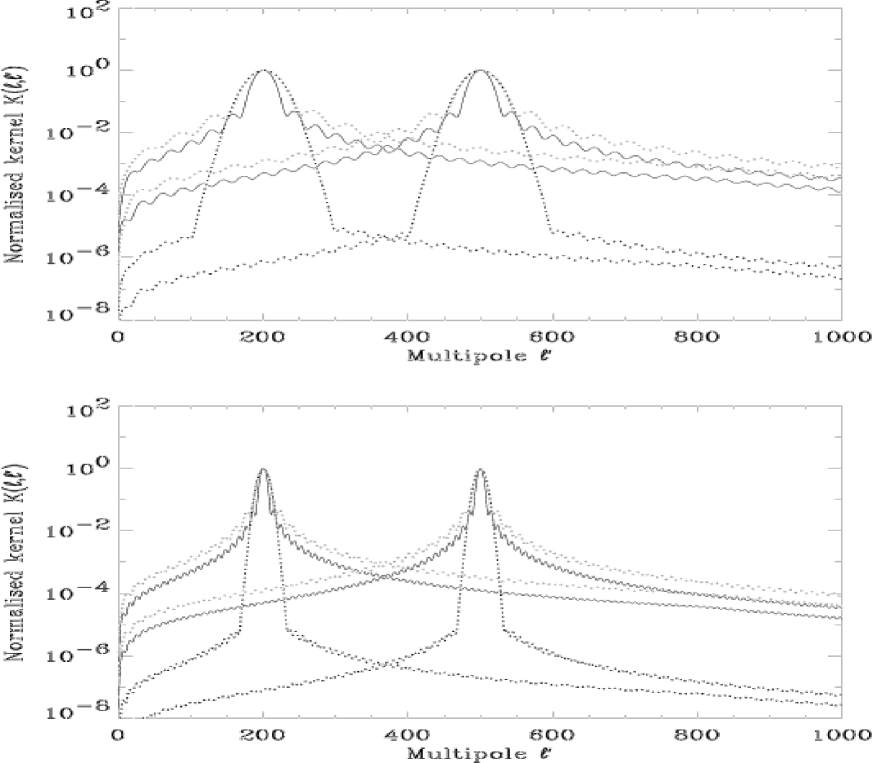
Figure 3: The figures show slices of the kernel $K(\ell,\ell^{\prime})$ connecting the full sky and cut sky spherical harmonic coefficients. The full kernels are shown in Figs. 1 and 2. The slices are taken at $\ell=200$ and $\ell=500$ for the 5 (upper plot) and 15 (lower plot) degree Gaussian Gabor window (dotted black line). The solid line is for the corresponding (same area on the sky) top-hat window $W_{\mathrm{A}}$. The dotted coloured line is for the top-hat window $W_{\mathrm{I}}$ having the same integrated area as the Gaussian window. The kernels are here normalised so that the peak in the given slice has its maximum at $1$. In this way one can easier compare the shape of the kernels.

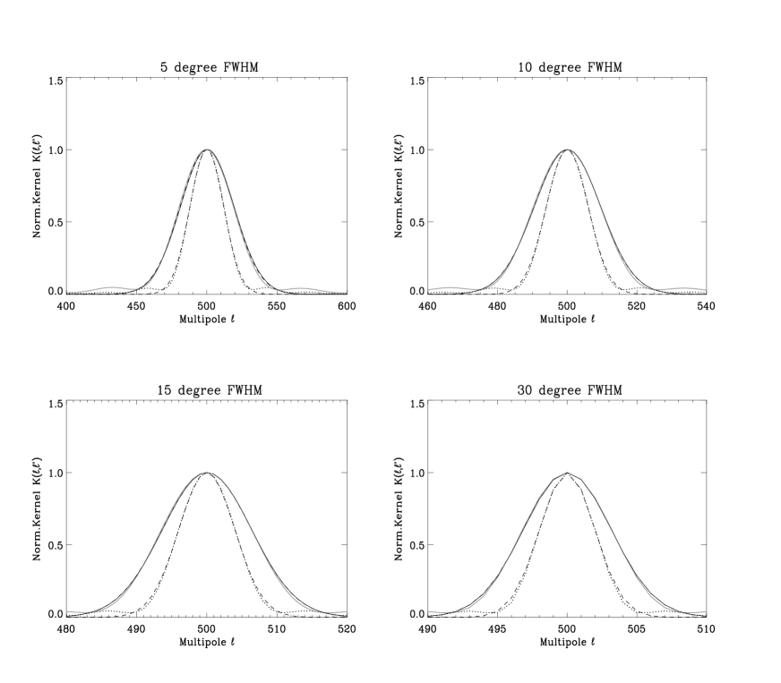
Figure 4: The figures show a slice of the kernel $K(\ell,\ell^{\prime})$ connecting the full sky and cut sky spherical harmonic coefficients. The slices are taken at $\ell=500$ for a $5$, $10$, $15$ and $30$ degree FWHM Gaussian Gabor window (solid line) with a $\theta_{\mathrm{C}}=3\sigma$ cut-off. The dotted line shows the kernel for a top-hat window $W_{\mathrm{A}}$ covering the same area on the sky. The coloured lines which are almost on top of the lines for the Gaussian Gabor windows show the kernels for a top-hat window $W_{\mathrm{I}}$ which has the same integrated area as the Gaussian windows $W_{\mathrm{G}}$. The dashed lines which are almost on top of the dotted and solid line (and for this reason not so easily seen in the plot) are Gaussian fits to the curves.

Figure 5: The figure shows the uncertainty relation $\Delta\ell\Delta\theta=\mathrm{constant}$ for a Gabor transform on the sphere. The solid line shows the width $\Delta\ell$ of the Gabor kernel $K(\ell,\ell^{\prime})$ connecting the full sky and the cut sky power spectra when applying a Gaussian Gabor window with a cut $\theta_{\mathrm{C}}=3\sigma$. The FWHM is shown on the lower abscissa. The dashed line shows the width of the kernel for a top-hat window. The full radius of the top-hat window is shown on the upper abscissa. The curves are well described by $\Delta\ell=220/\theta_{\mathrm{FWHM}}$ and $\Delta\ell=175/\theta_{\mathrm{radius}}$ for the Gaussian and top-hat windows respectively. As will be discussed in Section 3.2, this relation also describes the width of the correlation matrix of $\tilde{C}_{\ell}$. The width of the correlation matrix using a Gaussian window follows the relation in this plot times a factor $1.42$. For the top-hat window, the width of the correlation matrix is the same as for the kernel shown in this figure.

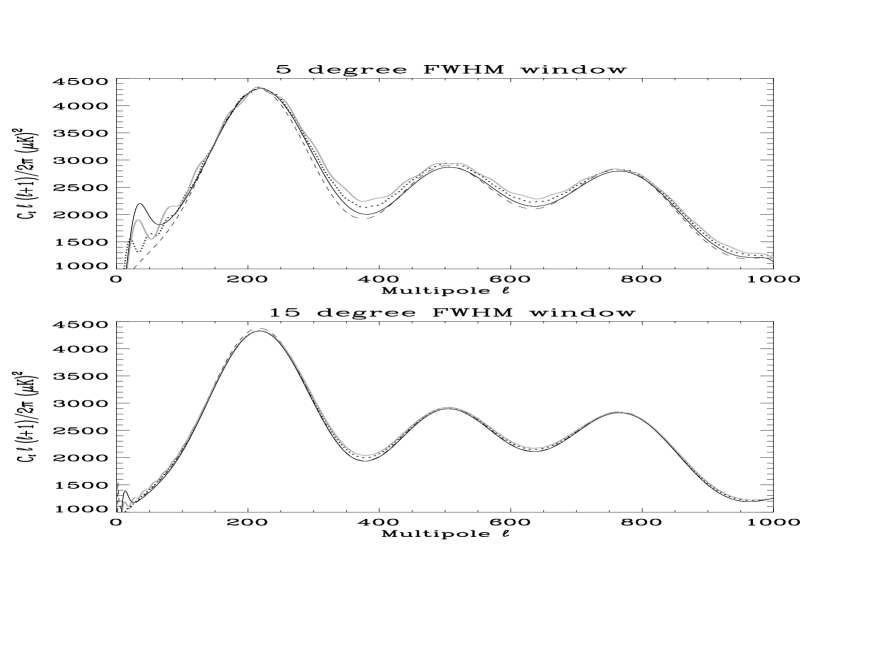
Figure 6: The windowed power spectra $\tilde{C}_{\ell}$ for a $5$ and $15$ degree FWHM Gaussian Gabor Gabor window $W_{\mathrm{G}}$ cut at $\theta_{\mathrm{C}}=3\sigma$ (solid line) and for a top-hat window $W_{\mathrm{A}}$ covering the same area on the sky (dotted line). The spectrum for the top-hat window $W_{\mathrm{I}}$ for which the integrated area of the window corresponds to the Gaussian is shown as a coloured line. All spectra are normalised in such a way that they can be compared directly with the full sky spectrum which is shown on each plot as a dashed line. Only in the first plot are all four lines visible. In the last plot, the full sky spectrum and the Gaussian pseudo spectrum (dashed and solid line) are only distinguishable in the first few multipoles.

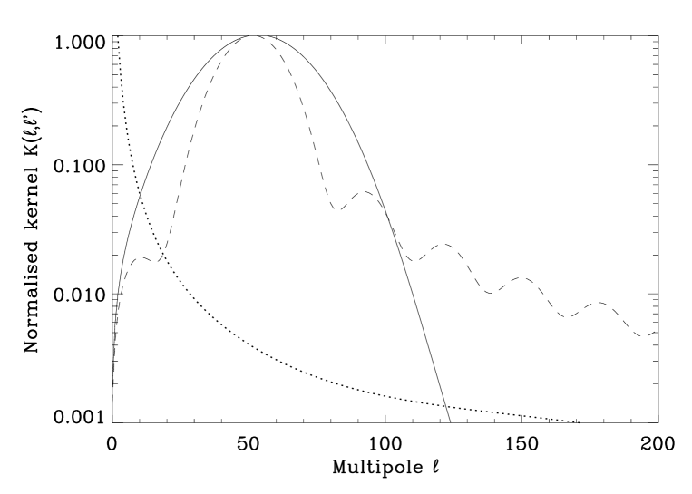
Figure 7: The figure shows a slice of the kernel $K(\ell,\ell^{\prime})$ connecting the full sky and cut sky spherical harmonic coefficients. The slice is taken at $\ell=50$ for a $5$ degree FWHM Gaussian Gabor window (solid line) and a corresponding top-hat window $W_{\mathrm{A}}$ (dashed line). The kernels are normalised to one at the peak. A typical power spectrum normalised to one at the quadrupole is plotted as a dotted line. The figure aims at explaining the extra peak in the pseudo power spectrum at low multipoles for the Gaussian Gabor window shown in Fig. 6.

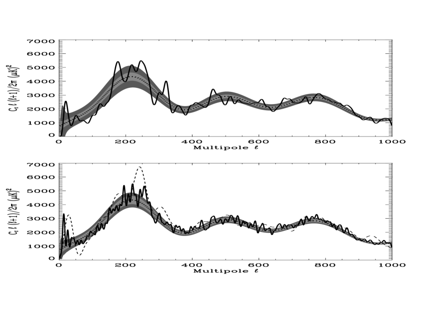
Figure 8: One realisation of the windowed power spectra. The upper plot shows a realisation of a pseudo power spectrum using a $15$ degree FWHM Gaussian Gabor window. The pseudo spectrum is normalised in such a way that it can be compared directly to the full sky spectrum which average is shown as a dotted line. The lower plot shows the same realisation using a corresponding top-hat window. The light shaded area shows $1\sigma$ cosmic variance around the full sky average spectrum. The darker area shows $1\sigma$ cosmic and sampling variance taken from the theoretical formula. On the lower plot, the pseudo spectrum with a top-hat window $W_{\mathrm{A}}$ having the same integrated area as in the upper plot is shown as a dashed line.

In Fig. 1 we have plotted the kernel for a Gaussian Gabor window,

$$G(\theta)= \mathrm{e}^{-\theta^{2}/(2\sigma^{2})} \theta\leq\theta_{\mathrm{C}},$$ (19)

$$G(\theta)= 0 \theta>\theta_{\mathrm{C}},$$ (20)

with $5$ and $15$ degrees FWHM (corresponding to $\sigma=2.12^{\circ}$ and $\sigma=6.38^{\circ}$) and $\theta_{\mathrm{C}}=3\sigma$. One sees that the kernel is centred about $\ell=\ell^{\prime}$, and falls off rapidly. Fig. (2) shows the same for the corresponding top-hat Gabor windows,

$$G(\theta)= 1 \theta\leq\theta_{\mathrm{C}},$$ (21)

$$G(\theta)= 0 \theta>\theta_{\mathrm{C}}.$$ (22)

The top-hat windows are covering the same area on the sky as the corresponding Gaussian windows in Fig. 1 ($\theta_{\mathrm{C}}$ is the same). Ones sees that the diagonal is broader for the smaller windows indicating stronger couplings. Another thing to notice is that whereas the kernel for the top-hat Gabor window only falls by about 4 orders of magnitude from the diagonal to the far off-diagonal elements, the Gaussian Gabor kernel falls by about 8 orders of magnitude (the vertical axis on the four plots are the same). The smooth cut-off of the Gaussian Gabor window cuts off long range correlations in spherical harmonic space. One of the aims of the first part of this paper is to see how the pseudo power spectrum of a given disc on the sky (top-hat window) is affected by the multiplication with a Gaussian Gabor window. For this reason the pseudo spectrum will be studied for a top-hat and a Gaussian covering the same area on the sky. We will also study a top-hat window which has the same integrated area as the Gaussian window. The cut-off angle $\theta_{\mathrm{C}}=\theta_{\mathrm{int}}$ for these windows is given by

$$\int_{\theta=0}^{\theta=3\sigma}G(\theta)d\cos\theta=\int_{\theta=0}^{\theta=\theta_{\mathrm{int}}}d\cos\theta.$$ (23)

In this section we will be comparing a Gaussian window (called $W_{\mathrm{G}}$) having $\theta_{\mathrm{C}}=3\sigma$ with a top-hat window (called $W_{\mathrm{A}}$) having the same area on the sky ($\theta_{\mathrm{C}}=3\sigma$) and with a top-hat window (called $W_{\mathrm{I}}$) having the same integrated area ($\theta_{\mathrm{C}}=\theta_{\mathrm{int}}$).

In Fig. 3, we have plotted slices of the kernel at $\ell=200$ and $\ell=500$ for the 5 and 15 degree FWHM Gaussian Gabor windows (dashed line). The solid line is the corresponding kernel (same area on the sky) when using the top-hat Gabor window ($W_{\mathrm{A}}$). One sees that the Gaussian window effectively cuts off long range correlations whereas the top-hat window is narrower close to the diagonal. The Gaussian window has larger short range correlations. The coloured lines show the slice of the kernel for a top-hat window having the same integrated area as the Gaussian window ($W_{\mathrm{I}}$). These kernels have the same widths as the kernels for the Gaussian windows, but the long range correlations are significantly larger. In [Hobson & Magueijo 1996] it was shown that in the flat-sky approximation, the long range correlations are significant when the window has a sharp cut-off. On the sphere we see that even for a sharp top-hat window the long range correlations are damped.

Fig. 4 shows how the width of the kernel gets narrower and the correlations smaller as the Gabor window opens up. The four kernels are shown for $\ell=500$ and the Gaussian windows have 5, 10, 15 and 30 degree FWHM with $\theta_{\mathrm{C}}=3\sigma$. The same kernels for the top-hat windows $W_{\mathrm{A}}$ (dotted lines) and $W_{\mathrm{I}}$ (coloured line) are plotted on top. Gaussian fits are plotted on top of the kernels and show that the kernels are very close to Gaussian functions near the diagonal.

In Fig. 5 we have plotted the relation between the FWHM width $\Delta\ell$ of the kernel and the size $\Delta\theta$ of the window for Gaussian and top-hat windows. The two curves are very well described by $\Delta\ell=220/\theta_{\mathrm{FWHM}}$ for the Gaussian window ($\theta_{\mathrm{FWHM}}$ in degrees) and $\Delta\ell=175/\theta_{\mathrm{radius}}$ ($\theta_{\mathrm{radius}}$ being the radius of the top-hat window in degrees) for the top-hat window. Clearly for a given observed area of the sky, multiplying with a Gaussian will increase the FWHM of the kernel. This is also what was seen in Figs 3 and 4. We will see that this results in a lower spectral resolution for the Gaussian window compared to the top-hat window. But the lower long range correlations of the Gaussian window makes the shape of the pseudo power spectrum closer to that of the full sky power spectrum.

In Fig. 6, we show the shapes of the $\tilde{C}_{\ell}$ for Gaussian and top-hat windows compared to the full sky spectrum. The plots which were made using the analytical formula (16) show $\tilde{C}_{\ell}$ for a $5$ and $15$ degree FWHM Gaussian Gabor window (solid line) cut at $3\sigma$. The corresponding spectrum for the top-hat Gabor window $W_{\mathrm{A}}$ is shown as dotted lines and for the top-hat window $W_{\mathrm{I}}$ as coloured lines. The spectra are normalised in such a way that they can be compared to the full sky power spectrum (dashed line). For the $5^{\circ}$ FWHM window one can still distinguish the four lines. At this window size the pseudo spectra are very similar to the full sky spectra but with small deviations depending on the shapes of the kernel and the shape of the power spectrum. In this case the spectrum for the Gaussian window seems to be smaller at the peaks and larger at the troughs whereas the spectrum for the top-hat windows is always larger.

For the $15^{\circ}$ FWHM windows the pseudo spectrum using the Gaussian Gabor window are on top of the full sky power spectrum. For the top-hat windows it is still possible to distinguish the pseudo spectrum from the full sky power spectrum although the lines are still very close. The plot implies that the $\tilde{C}_{\ell}$ could be good estimators of the underlying full sky $C_{\ell}$ provided that the window is big enough. Note that for small windows, the Gaussian Gabor window makes the pseudo spectrum a better estimator than the pseudo-spectrum for a top-hat window at higher multipoles. In [Hobson & Magueijo 1996] it was shown in the flat-sky approximation that the pseudo power spectrum for small fields get significantly distorted, but that the shape of the pseudo spectrum gradually approaches the shape of the full sky power spectrum when the window gets larger. We see here that the same results applies to the treatment on the sphere. In the flat-sky approximation however, the error in estimating the average power spectrum from the pseudo power spectrum from one single realisation is bigger due to the long range correlations of the pseudo power spectrum coefficients in the flat-sky approximation.

One feature which is very prominent is the additional peak at low $\ell$ for the Gaussian window. The reason for this peak comes from the fact that the diagonal in the Gaussian kernel is broader than in the top-hat kernel for a top-hat window with corresponding area. For the low multipoles the power spectrum is dropping rapidly because of the Sachs-Wolfe effect and the lowest multipole $C_{\ell}$ are much bigger than the $C_{\ell}$ for higher multipoles. Since the Gaussian kernel is broad, the $\tilde{C}_{\ell}$ at low multipoles will pick up more from the $C_{\ell}$ at lower multipoles than the narrower top-hat kernel (see Fig. 3). These low multipole $C_{\ell}$ have very high values compared to the higher multipole $C_{\ell}$ and for that reason the $\tilde{C}_{\ell}$ for the Gaussian window will get a higher value. This is illustrated in Fig. 7 where a slice of the kernel at $\ell=50$ is shown for the $5^{\circ}$ FWHM Gaussian Gabor window (solid line) and the corresponding top-hat $W_{\mathrm{A}}$ (dashed line) normalised to one at the peak. The dotted line shows a typical power spectrum. Clearly the Gaussian kernel will pick up more of the high value $C_{\ell}$ at low multipoles. Note that for the pseudo spectrum for the top-hat window $W_{\mathrm{I}}$ where the integral of the top-hat window corresponds to the integrated Gaussian window (coloured line), there is also a peak at low multipole. The reason is that the width of the kernel is the same as for the Gaussian.

In Fig. 8 we show the pseudo power spectra for a particular realisation using a $15$ degree FWHM Gaussian window (upper plot) and a top-hat window $W_{\mathrm{A}}$(lower plot). The pseudo spectra are compared to the average full sky spectra shown as a dashed line. The dark shaded area shows the expected $1\sigma$ cosmic and sample variance on the pseudo spectra taken from the formulae to be developed in the next sections. The lighter shaded area shows only cosmic variance. Note that the pseudo spectrum for the Gaussian window is smoother than the pseudo spectrum for the top-hat window. This shows the lower spectral resolution of the Gaussian window due to the broader kernel.

3 Likelihood Analysis

In this section we will show how the pseudo power spectrum can be used as input to a likelihood analysis for estimating the full sky power spectrum from an observed disc on the sky multiplied with a Gabor window. We will in this section concentrate on a Gaussian Gabor $W_{\mathrm{G}}$ window, but the formalism is valid for any azimuthally symmetric Gabor window. We start by showing that the pseudo-$C_{\ell}$ are close to Gaussian distributed which allows for a Gaussian form of the likelihood function. Then we show how the correlation matrices can be calculated quickly for an axisymmetric patch on the sky with uncorrelated noise. The extension to the more realistic situation with correlated noise and non-axisymmetric sky patches will be made in the next section. We will show the results of power spectrum estimations with different noise profiles and window sizes. We will also show that the use of a window different from the top-hat window can be advantageous for some noise profiles, even if the window has a lower spectral resolution than the top-hat window.

3.1 The form of the likelihood function

To know the form of the likelihood function, one needs to know the probability distribution of $\tilde{C}_{\ell}$. In Figs 9 and 10 we show the probability distribution from 10000 simulations with a $5^{\circ}$ and $15^{\circ}$ FWHM Gaussian Gabor window respectively. The dashed line shows a Gaussian with mean value and standard deviation found from the formulae given in the previous and next section. One can see that the probability distribution is slightly skewed for low $\ell$, but for high $\ell$ it seems to be very well approximated by a Gaussian. Also the small window shows more deviations from a Gaussian than the bigger window. In Fig. 11 we show that this result is not limited to the Gaussian window. The plot shows the probability distribution from a simulation with a top-hat Gabor window $W_{\mathrm{A}}$ covering the same area on the sky as the $15^{\circ}$ FWHM Gaussian window. Also for this window the probability distribution is close to Gaussian.

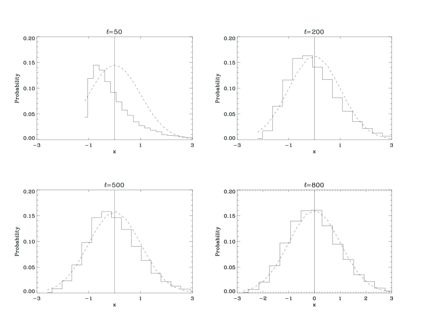
Figure 9: The probability distribution of $\tilde{C}_{\ell}$ taken from 10000 simulations with a $5^{\circ}$ FWHM Gaussian Gabor window truncated at $\theta_{\mathrm{C}}=3\sigma$. The variable $x$ is given as $x=(\tilde{C}_{\ell}-\langle\tilde{C}_{\ell}\rangle)/\sqrt{\langle(\tilde{C}_{\ell}-\langle\tilde{C}_{\ell}\rangle)^{2}\rangle}$. The dashed line is a Gaussian with the theoretical mean and standard deviation of the $\tilde{C}_{\ell}$. The plot shows the $\tilde{C}_{\ell}$ distribution for $\ell=50$, $\ell=200$, $\ell=500$, and $\ell=800$. The probabilities are normalised such that the integral over $x$ is $1$.

Figure 10: Same as Fig. 9 but for a $15^{\circ}$ FWHM Gaussian Gabor window.

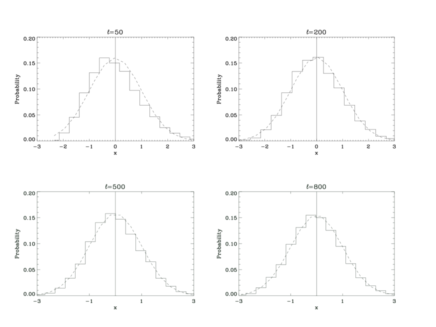
Figure 11: Same as Fig. 10 but for a top-hat Gabor window $W_{\mathrm{A}}$ covering the same area on the sky.

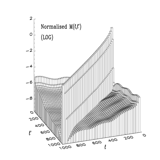
Figure 12: The figure shows the correlation matrix $M_{\ell\ell^{\prime}}$ between pseudo spectrum coefficients normalised with the pseudo spectrum $(\langle\tilde{C}^{\mathrm{T}}_{\ell}\tilde{C}^{\mathrm{T}}_{\ell^{\prime}}\rangle-\langle\tilde{C}^{\mathrm{T}}_{\ell}\rangle\langle\tilde{C}^{\mathrm{T}}_{\ell^{\prime}}\rangle)/(\langle\tilde{C}^{\mathrm{T}}_{\ell}\rangle\langle\tilde{C}^{\mathrm{T}}_{\ell^{\prime}}\rangle)$ for a 15 degree FWHM Gaussian Gabor window. A standard CDM power spectrum was used to produce this matrix.

Figure 13: The analysis of an input model with $\Omega_{\mathrm{total}}=1$, $\Omega_{\Lambda}=0.7$, $\Omega_{\mathrm{b}}h^{2}=0.03$ and $n_{\mathrm{s}}=0.975$. We used a non-uniform white noise model with $S/N=1$ at $\ell=575$. The dotted line is the input average full sky power spectrum and the histogram shows the binned pseudo power spectrum for this realisation (without noise). We used $N^{\mathrm{bin}}=20$ bins and $N^{\mathrm{in}}=100$ input sample points to the likelihood. The shaded areas around the binned average full sky spectrum (which is not plotted) are the theoretical variance with and without noise. The bright shaded area shows cosmic and sample variance and the dark shaded area also has variance due to noise included. The variance due to noise was calculated using formula (32) for uniform noise. The $1\sigma$ error bars on the estimates are taken from the inverse Fisher matrix. The solid line increasing from the left to the right is the noise power spectrum.

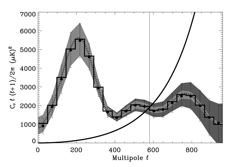
Figure 14: Same as in Fig. 13 but this is an average over 1000 simulations and estimations. The histogram is now the binned average full sky power spectrum. The error bars on this plot are the $1\sigma$ variances taken from Monte Carlo.

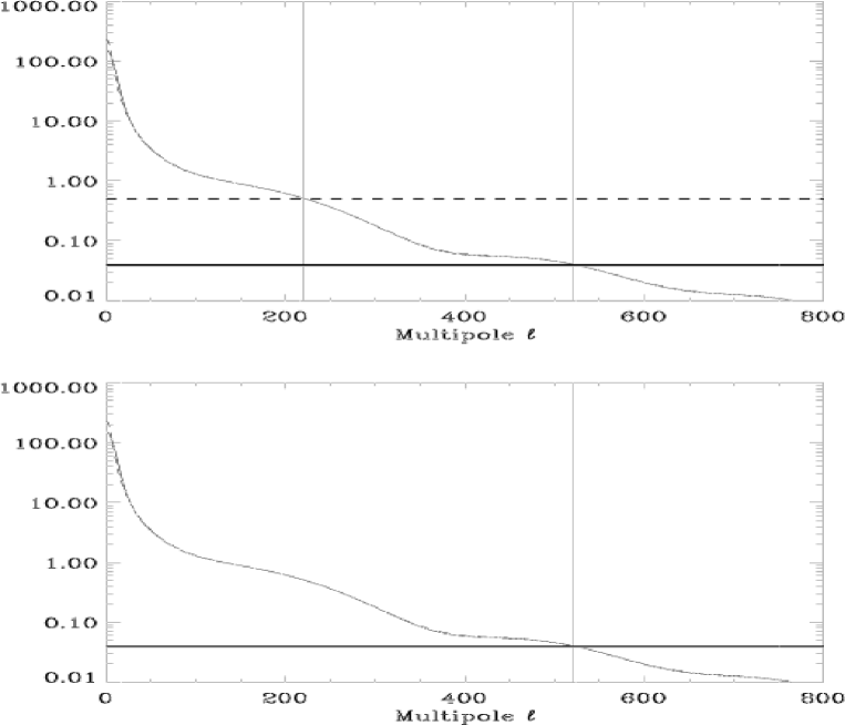
Figure 15: The plots show average signal and noise pseudo power spectra plotted separately. The spectra are normalised so that they can be compared to the full sky power spectrum. The solid and dashed curves which almost fall together are the signal pseudo power spectra for a $15$ degree FWHM Gaussian Gabor window $W_{\mathrm{G}}$ and a corresponding top-hat window $W_{\mathrm{A}}$ respectively. In the upper plot the noise model shown in Fig. 16 was used. This noise model is increasing from the north pole and down to the edges of the patch. This is opposite of the Gaussian window and for this reason the Gaussian window gets higher signal to noise ratio. The solid horizontal line in the upper plot shows the noise pseudo power spectrum for the Gaussian window and the dashed horizontal line shows the noise pseudo power spectrum for the top-hat window. In the lower plot a uniform noise model was used so that the noise pseudo power spectra fall together and are shown as a solid vertical line. The figure shows how a Gabor window different from a top-hat can be used to increase signal to noise.

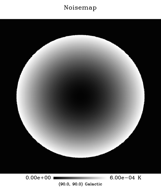
Figure 16: The noise map with noise increasing from the north pole and downwards. The figure shows a gnomic projection with the north pole in the centre.

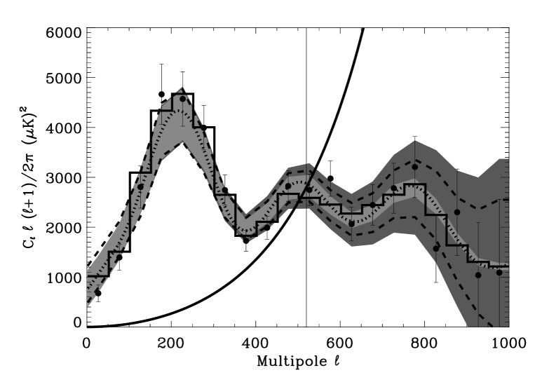
Figure 17: Same as Fig. 13 but for a standard CDM model. The noise is increasing from the centre and out to the edges while the Gaussian Gabor window has the opposite effect, giving an increased significance to pixels with less noise. As in Fig. 13 the shaded areas show the analytically calculated variance using the ‘naive’ formula for the uniform noise case. The dashed lines show the expected variance using the inverse of the Fisher matrix.

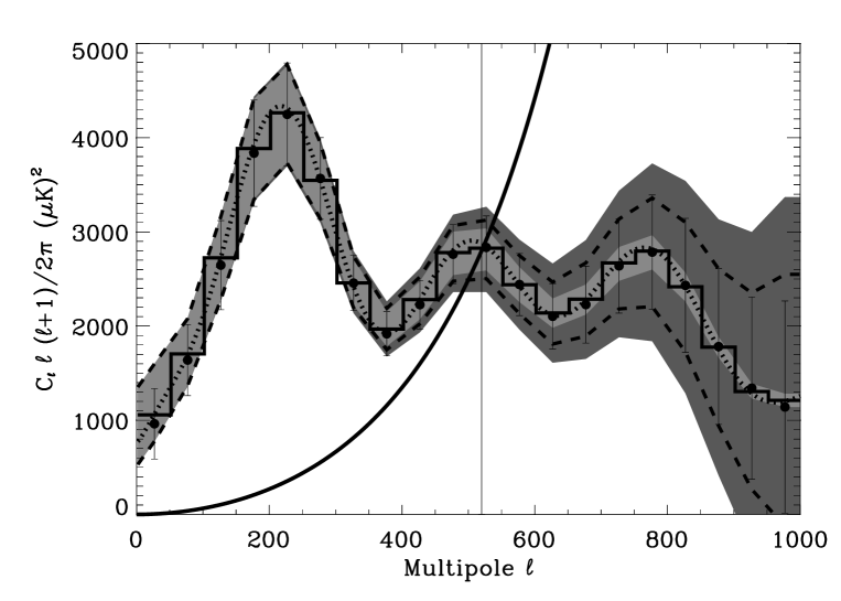
Figure 18: Same as Fig. 17 but with 5000 simulations and estimations averaged. The histogram now shows the binned average full sky power spectrum. The error bars on the estimates are here the $1\sigma$ averages from Monte Carlo.

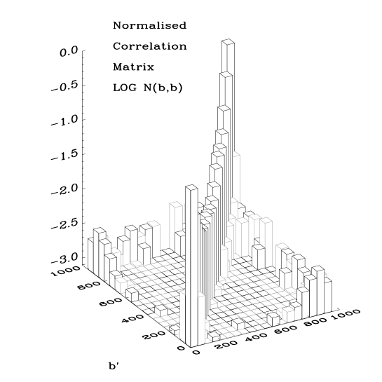
Figure 19: The average correlation matrix $N(b,b^{\prime})\equiv\langle D_{b}D_{b^{\prime}}\rangle/(\langle D_{b}\rangle\langle D_{b^{\prime}}\rangle)-1$ of the estimates in Fig. 18. The negative elements are coloured.

Figure 20: The probability distribution of the estimates $D_{b}$ in Fig. 18. The variable $x$ is given as $x=(D_{b}-\langle D_{b}\rangle)/\sqrt{\langle(D_{b}-\langle D_{b}\rangle)^{2}\rangle}$. The dashed line is a Gaussian with mean and standard deviation taken from Monte Carlo. The plot shows bin estimates centred at $\ell=225$, $\ell=425$, $\ell=525$ and $\ell=725$.

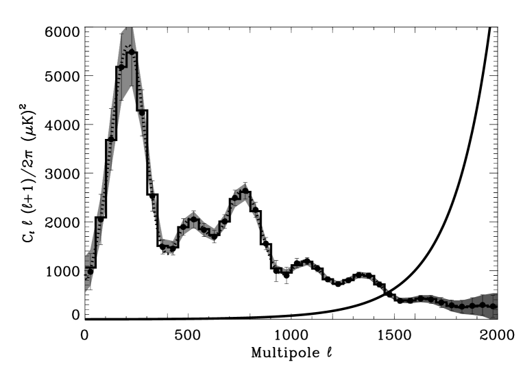
Figure 21: Same as Fig. 14 for $100$ simulations where the beam and noise level was set according to the specifications of the Planck $143\mathrm{GHz}$ channel. Again a $15^{\circ}$ FWHM Gaussian Gabor window was used. The power spectrum was estimated in $40$ bins between $\ell=2$ and $\ell=2048$

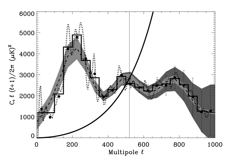
Figure 22: The average of 300 estimations where the input $\tilde{C}_{\ell}$ were taken from simulations with a fixed CMB realisation but varying noise realisations. The dotted line is the $N^{\mathrm{in}}$ input $\tilde{C}_{\ell}$ from the CMB realisation without noise. The histogram is the same spectrum binned in $N^{\mathrm{bin}}$ bins. The dashed line is the binned average full sky power spectrum from which this realisation was made. The shaded areas around the binned full sky spectrum show the variance with (dark) and without (bright) noise. The solid line rising from the left to the right is the noise power spectrum.

From the above plots it seems to be reasonable to approximate the likelihood function with a Gaussian provided the window is big enough and multipoles at high enough $\ell$ values are used,

$$\mathcal{L}=\frac{\mathrm{e}^{-\frac{1}{2}{\mathbf{d}}^{\mathrm{T}}{\mbox{$\textbf{{M}}$}}^{-1}{\mathbf{d}}}}{\sqrt{2\pi\det{\mbox{$\textbf{{M}}$}}}}.$$ (24)

Omitting all constant terms and factors, the log-likelihood can then be written:

$$L={\mathbf{d}}^{\mathrm{T}}{\mbox{$\textbf{{M}}$}}^{-1}{\mathbf{d}}+\ln{\det{{\mbox{$\textbf{{M}}$}}}}.$$ (25)

Here ${\mathbf{d}}$ is the data vector vector which contains the observed $\tilde{C}_{\ell}$ for the set of sample $\ell$-values $\ell_{i}$. The data is taken from the observed windowed sky in the following way:

$$d_{i}=\tilde{C}_{\ell_{i}}-\langle\tilde{C}_{\ell_{i}}\rangle.$$ (26)

The matrix M is the covariance between pseudo-$C_{l}$ which elements are given by:

$$M_{ij}=\langle\tilde{C}_{\ell_{i}}\tilde{C}_{\ell_{j}}\rangle-\langle\tilde{C}_{\ell_{i}}\rangle\langle\tilde{C}_{\ell_{j}}\rangle.$$ (27)

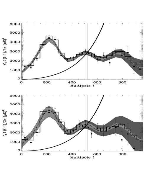
Figure 23: Estimates of $\tilde{C}_{\ell}$ using a Gaussian Gabor window (lower plot) and a top-hat window (upper plot). Here we used a uniform noise model with $S/N=1$ at $\ell=520$. The dotted line shows the average full sky power spectrum and the histogram shows the input pseudo power spectrum without noise for this realisation, binned in the same way as the estimates. The bright shaded area shows the cosmic and sample variance around the binned average spectrum (not plotted). The dark shaded area has the variance due to noise included. The $1\sigma$ error bars on the estimates are taken from the inverse Fisher matrix. The solid line increasing from left to right is the noise power spectrum.

In Appendix (E) and (F) we have found expressions which enable fast evaluations of $d_{i}$ and $M_{ij}$ for signal and noise. These major results are are given in equations (87), (102) and (110) and the recursion which enables fast calculation of these expressions is given in equation (C). In the derivations of the expressions for $M_{ij}$, the rotational invariance of the (not-averaged) $\tilde{C}_{\ell}$ shown in Appendix (D) was used. Because of this rotational invariance, all derivations can be done with the Gabor window centred at the north pole. In Fig. 12 we used the full formula (equation 87) from Appendix (E) to calculate the signal correlation matrix for a typical power spectrum with a $15^{\circ}$ FWHM Gaussian Gabor window (note that in the figure, the correlation matrix is normalised with the pseudo power spectrum). The correlation between $\tilde{C}_{\ell}$ of different multipoles is falling of rapidly with the distance from the diagonal. Only exception being the small ’wall’ at low multipoles which again comes from the coupling to the smallest multipoles which have very high values.

3.2 Likelihood estimation and results

Because of the limited information content in one patch of the sky one can not estimate the full sky $C_{\ell}$ for all multipoles $\ell$. For this reason the full sky power spectrum has to be estimated in $N^{\mathrm{bin}}$ bins. Also the algorithm to minimise the log-likelihood needs the different numbers to be estimated to be of roughly the same order of magnitude. For this reason we estimate for some parameters $D_{b}$ which for bin $b$ is defined as

$$C_{\ell}=\frac{D_{b}}{\ell(\ell+1)},\ \ \ell_{b}\leq\ell<\ell_{b+1},\\$$ (28)

where $\ell_{b}$ is the first multipole in bin $b$.

Since the $\tilde{C}_{\ell}$ are coupled, one can not use all multipoles in the data vector, the covariance matrix would in this case become singular. One has to choose a number $N^{\mathrm{in}}$ of multipoles $\ell_{i}$ for which one finds $d_{i}$. How many multipoles to use depends on how tight the $\tilde{C}_{\ell}$ are coupled which depends on the width $\Delta\ell_{\mathrm{kern}}$ of the kernel (Fig. 5) or the width $\Delta\ell_{\mathrm{cor}}$ of the correlation matrix. The width of the correlation matrix(normalised with the psuedo power spectrum) varies with window size in the same way as the width of the kernel varies with window size. In fact for the top-hat window these two widths are the same and for the Gaussian window we found that $\Delta\ell_{\mathrm{cor}}\approx 1.42\Delta\ell_{\mathrm{kern}}$. The optimal number of $N^{\mathrm{in}}$ to use seems to be $N^{\mathrm{in}}\approx 3/2\ \ell_{\mathrm{max}}/\Delta\ell_{\mathrm{kern}}$. To use a lower $N^{\mathrm{in}}$ increases the error bars on the estimates and a higher $N^{\mathrm{in}}$ does not improve the estimates. One can at most fit for as many $C_{\ell}$s as the number of $\tilde{C}_{\ell}$ ($N^{\mathrm{in}}$) one has used in the analysis. So one needs to find a number $N^{\mathrm{bin}}\leq N^{\mathrm{in}}$ of bin values $D_{b}$ from which one can construct the full sky power spectrum $C_{\ell}$.

In Appendix (E) and (F) we found that the full correlation matrix can be written as

$$M_{ij}=M_{ij}^{\mathrm{S}}+M_{ij}^{\mathrm{N}}+M_{ij}^{\mathrm{X}},$$ (29)

where $M_{ij}^{\mathrm{N}}$ is the noise correlation matrix which has to be precomputed for a specific noise model (analytically or by Monte Carlo as will be shown in Section (4)). The signal and signal-noise cross correlation matrices are on the form

$$M^{\mathrm{S}}_{ij} = \sum_{b}\sum_{b^{\prime}}D_{b}D_{b^{\prime}}\chi(b,b^{\prime},i,j),$$ (30)

$$M^{\mathrm{X}}_{ij} = \sum_{k}D_{b}\chi^{\prime}(b,i,j),$$ (31)

where the $\chi$-functions can be precomputed using formulae (89) and (115).

We will now describe some test simulations to show how the method works. As a first test, we used the same model as was used in [Hivon et al. 2002], with $\Omega_{\mathrm{total}}=1$, $\Omega_{\Lambda}=0.7$, $\Omega_{\mathrm{b}}h^{2}=0.03$ and $n_{\mathrm{s}}=0.975$. These are the parameters from the combined Maxima-Boomerang analysis [Jaffe et al. 2001]. We used a circular patch with $15.5^{\circ}$ radius covering the same fraction of the sky as in [Hivon et al. 2002]. Using HEALPix we simulated a CMB sky using a standard CDM power spectrum with $l_{\mathrm{max}}=1024$ and a $7^{\prime}$ pixel size ($N_{\mathrm{side}}=512$ in HEALPix language). We smoothed the map with a $10^{\prime}$ beam and added non-correlated non-uniform noise to it. Here a Gaussian Gabor window with $FWHM=12^{\circ}$ was used with a cut-off $\theta_{\mathrm{C}}=3\sigma$. For the likelihood estimation, we had $N^{\mathrm{bin}}=20$ full sky $C_{\ell}$ bins and $N^{\mathrm{in}}=100$ $\tilde{C}_{\ell}$ values between $\ell=2$ and $\ell=960$. In Fig. 13 one can see the result. The shaded areas are the expected $1\sigma$ variance with and without noise. These were found from the theoretical formula

$$\Delta C_{b}=\sqrt{\frac{2}{\nu_{b}}}(C_{b}+N_{b}),$$ (32)

where $N_{b}$ is the noise ‘on the sky’, $\nu_{b}$ is the effective number of degrees of freedom given as

$$(2\ell_{b}+1)\Delta\ell f_{\mathrm{sky}}\frac{w_{2}^{2}}{w_{4}},$$ (33)

and the $w_{i}$ factors are dependent on the window according to

$$f_{\mathrm{sky}}w_{i}=\frac{1}{4\pi}\int_{4\pi}d{\hat{\mathbf{n}}}G^{i}({\hat{\mathbf{n}}}).$$ (34)

This formula is exact for a uniform noise model [Hivon et al. 2002] and is similar to the one used in most publications. It is in this case a very good approximation even with non-uniform noise. In the next example however we will show that the formula has to be used with care. In the figure, the error bars on the estimates are taken from the Fisher matrix and the signal-to-noise ratio $S/N=1$ at $\ell=575$.

In Fig. 14, we have plotted the average of 1000 such simulations, with different noise and sky realisations. From the plot, the method seems to give an unbiased estimate of the power spectrum bins $D_{b}$. For the lowest multipoles the estimates are slightly lower than the binned input spectrum. This is a result of the slightly skewed probability distribution of $\tilde{C}_{\ell}$ for small windows at these low multipoles (see Figs 9 and 10). The probability that the $\tilde{C}_{\ell}$ at lower multipoles have a value lower than the average $\langle\tilde{C}_{\ell}\rangle$ is high and the assumption about a Gaussian distribution about this average leads the estimates to be lower. When a bigger area of the sky is available such that several patches can be analysed jointly to give the full sky power spectrum, this bias seems to disappear. This will be shown in Section (4.1).

In this example one can see that the $1\sigma$ error bars from Monte Carlo coincide very well with the theoretical error shown as shaded areas from the formula in [Hivon et al. 2002]. Note that the error bars on the higher $\ell$ are smaller than in [Hivon et al. 2002] because the noise model used in that paper was not white. Also they took into account errors due to map making which is not considered here.

As a next test, we used a simulation with the same resolution and beam size. The power spectrum was this time a standard CDM power spectrum. We used an axisymmetric noise model with noise increasing from the centre and outwards to the edges (see Fig. 16). This is the kind of noise model which could be expected from an experiment scanning on rings, with the rings crossing in the centre. We now use a circular patch with $18.5^{\circ}$ radius and a $FWHM=15^{\circ}$ Gaussian Gabor window cut at $\theta_{\mathrm{C}}=3\sigma$. An interesting point now is that the Gabor window is decreasing from the centre and outwards, which is opposite of the noise pattern. This gives the pixels with low noise high significant in the analysis and the pixels with high noise low significance. One sees from the expressions for the signal and noise pseudo power spectra that the Gabor window will work differently on both. This means that $S/N$ is different depending on the Gabor window. For this case, we have plotted the average pseudo power spectrum for signal and noise separately in Fig. 15. This shows the described effect. The $S/N$ ratio is much higher for the Gaussian Gabor window in this case, favouring the use of this window for the analysis.

For this example we used again $N^{\mathrm{bin}}=20$ and $N^{\mathrm{in}}=100$. The result is shown in Fig. 17. In Fig. 18 the average over 5000 simulations and estimations is shown. One can see that the estimate also does well beyond $\ell=520$ which is where the effective $S/N=1$. The method is still unbiased. The error bars in the part where noise dominates are here lower than the theoretical approximation (32) shown as the dark shaded area. The dashed lines show the theoretical $1\sigma$ variance taken from the inverse Fisher matrix which here gives a very good agreement with Monte Carlo.

In Fig. 19 we show the average (over 5000 estimations) of the correlation between the estimates $D_{b}$ between different bins. The figure shows that the correlations between estimates are low and in fact in each line all off-diagonal elements are more than an order of magnitude lower than the diagonal element of that line. In Fig. 20 we show that the probability distribution of the estimates in Fig. 18 is almost Gaussian.

To test the method at higher multipoles we also did one estimation up to multipole $\ell=2048$. We used HEALPix resolution $N_{\mathrm{side}}=1024$ and simulated a sky with a $8^{\prime}$ Gaussian beam and added noise from a strongly varying non-uniform noise model. Both the beam and noise level were adjusted according to the specifications for the Planck HFI $143\mathrm{GHz}$ detector [Bersanelli et al. 1996]. We used again a $15^{\circ}$ FWHM Gaussian Gabor window cut $3\sigma$ away from the centre. In the estimation we used $N^{\mathrm{bin}}=40$ bins and $N^{\mathrm{in}}=200$ input $\tilde{C}_{\ell}$ between $\ell=7$ and $\ell=2048$. The average of 100 such simulations is shown in Fig. 21. Each complete likelihood estimation (which includes a total of about $25$ likelihood evaluations) took about $8$ minutes on a single processor on a $500\mathrm{MHz}$ DEC Alpha work station.

In Fig. 22, we have plotted the average of 300 estimations where the input data was the $\tilde{C}_{\ell}$ from simulations with a fixed CMB realisation and varying noise realisation. The dotted line shows the $N^{\mathrm{in}}$ $\tilde{C}_{\ell}$s (without noise) used as input to the likelihood. The histogram is as before the input pseudo spectrum without noise binned in $N^{\mathrm{bin}}$ bins. This means that each histogram line shows the average of the dotted line over the bin. One can see that the estimated power spectrum is partly following the $N^{\mathrm{in}}$ input $\tilde{C}_{\ell}$ and partly the binned power spectrum.

Finally, we made a comparison between a top-hat window and a Gaussian Gabor window. In this case we used uniform noise, so that the Gaussian and top-hat Gabor windows have the same $S/N$ ratio which we set to $1$ at $\ell=520$. We used a disc with $18^{\circ}$ radius, $N^{\mathrm{in}}=200$ and $N^{\mathrm{bin}}=20$. In Fig. 23 one can see the result. The lower plot shows the estimates with the Gaussian Gabor window ($15^{\circ}$ FWHM) and the upper with the top-hat window. The Gaussian window is suppressing parts of the data and for this reason gets a higher sample variance than the top-hat. This effect is seen in the plot. Clearly when no noise weighting is required the top-hat window seems to be the preferred window (which was also discussed in [Hivon et al. 2002]). This chapter has been concentrating on the Gaussian window to study power spectrum estimation in the presence of a window different from a top-hat. It has been shown that a different window can be advantageous when the noise is not uniformly distributed as one can then give data with different quality different significance.

4 Extensions of the Method

A real CMB experiment usually does not observe an axisymmetric patch of the sky. Usually the noise between pixels is also correlated. In order to take these two issues into account we will discuss two extensions of the method. The formalism for the extensions are worked out and some simple examples are shown. Further investigations of these extensions are left for a future paper, where the analysis of MAP and Planck data will be discussed. To be able to analyse non-axisymmetric parts of the sky, we propose to split the area up into several axisymmetric pieces and use the pseudo-$C_{\ell}$ from all these patches in the data vector of the likelihood and in this way analyse all patches jointly. We show that if the patches are not overlapping, the correlation between pseudo-$C_{\ell}$ from different patches is so weak that it can be neglected. To deal with correlated noise, we propose to use Monte Carlo simulations to find the noise correlation matrix. We demonstrate that for uncorrelated noise, one needs a few thousand simulations in order for the error bars on the $C_{\ell}$ estimates not to get larger than when using the analytic expression.

4.1 Multiple patches

It has been shown how one can do power spectrum estimation on one axisymmetric patch on the sky. The next question that arises is what to do when the observed area on the sky is not axisymmetric. In this case one can split the area into several axisymmetric pieces and use the $\tilde{C}_{\ell}$ from each piece. Then the $\tilde{C}_{\ell}$ from all the patches are used together in the likelihood maximisation. The first thing to check before embarking on this idea is the correlation between $\tilde{C}_{\ell}$s in different patches. In Appendix (H) the analytical formula for the correlation matrix describing the correlations between $\tilde{C}_{\ell}$ for different patches was derived (equation 131 and 135). With these expressions we can check how the correlations decrease as the distance between the two patches increase.

After the expression (131) was tested with Monte Carlo simulations, we computed the correlations between $\tilde{C}_{\ell}$ for two patches $A$ and $B$ where we varied the distance $\theta$ between the centres of $A$ and $B$. We used a standard CDM power spectrum and both patches $A$ and $B$ had a radius of $18^{\circ}$ apodised with a $15^{\circ}$ FWHM Gaussian Gabor window. In Fig. 24 we have plotted the diagonal of the normalised correlation matrix $(\langle\tilde{C}_{\ell}^{\mathrm{A}}\tilde{C}_{\ell}^{\mathrm{B}}\rangle-\langle\tilde{C}_{\ell}\rangle^{2})/\langle\tilde{C}_{\ell}\rangle^{2}$. The angels $\theta$ we used were $6^{\circ}$, $12^{\circ}$, $24^{\circ}$, $30^{\circ}$, $36^{\circ}$ and $180^{\circ}$. One sees clearly how the correlations drop with the distance. In the two last cases there were no common pixels in the patches. As one could expect, the correlations for the largest angels (the first few multipoles) do not drop that fast.

Figure 24: The correlation between $\tilde{C}_{\ell}$ between two patches $A$ and $B$ with an angular distance $\theta$ between the centres. A normal CDM power spectrum was used and the patches had an $18^{\circ}$ radius apodised with a $15^{\circ}$ FWHM Gaussian Gabor window. The figure shows the diagonal of the normalised correlation matrix $(\langle\tilde{C}_{\ell}^{\mathrm{A}}\tilde{C}_{\ell}^{\mathrm{B}}\rangle-\langle\tilde{C}_{\ell}\rangle^{2})/\langle\tilde{C}_{\ell}\rangle^{2}$ where of course $\langle C_{\ell}\rangle=\langle C_{\ell}^{\mathrm{A}}\rangle=\langle C_{\ell}^{\mathrm{B}}\rangle$ The angles used are (from top to bottom on the figure) $0^{\circ}$, $6^{\circ}$, $12^{\circ}$, $18^{\circ}$, $30^{\circ}$, $36^{\circ}$ and $180^{\circ}$.

In Fig. 25 we have plotted two slices of the correlation matrix of $\tilde{C}_{\ell}$ for a single patch at $\ell=400$ and $\ell=800$. On the top we plotted the diagonals of the correlation matrices for separation angle $\theta=30^{\circ}$, $\theta=36^{\circ}$ and $\theta=180^{\circ}$. One sees that for the case where the patches do not have overlapping pixels, the whole diagonals have the same level as the far-off-diagonal elements in the $\theta=0^{\circ}$ matrix. When doing power spectrum estimation on one patch, the result did not change significantly when these far-off-diagonal elements were set to zero. For this reason one expects that when analysing several patches which do not overlap, simultaneously, the correlations between non-overlapping patches do not need to be taken into account. Note however that for the $\theta=30^{\circ}$ which means that there are only a few overlapping pixels, the approximation will not be that good as the level is orders of magnitude above the far-off-diagonals of the $\theta=0^{\circ}$ matrix. Another thing to note is that for the lowest multipoles, the correlation between patches is still high but we will also assume this part to be zero and attempt a joint analysis of non-overlapping patches.

Figure 25: slices of the correlation matrices which diagonals are shown in Fig. 24. The solid lines (thin and thick) show a slice of the $\theta=0^{\circ}$ correlation matrix at $\ell=400$ and $\ell=800$ respectively. The dashed lines (thin and thick) show the diagonal of the correlation matrices for $\theta=36^{\circ}$ and $\theta=30^{\circ}$ respectively. The dotted line is the diagonal of the $\theta=180^{\circ}$ matrix.

The full correlation matrices for $0$ and $30$ degree separation are shown in Fig. 26. The figures show how the diagonal is dropping relative to the far off-diagonal elements.

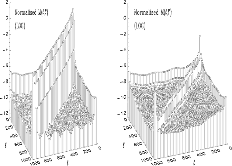
Figure 26: The figure shows the normalised correlation matrices $M(\ell,\ell^{\prime})=(\langle C^{\mathrm{A}}_{\ell}C^{\mathrm{B}}_{\ell}\rangle-\langle C^{\mathrm{A}}_{\ell}\rangle\langle C^{\mathrm{B}}_{\ell}\rangle)/(\langle C^{\mathrm{A}}_{\ell}\rangle\langle C^{\mathrm{N}}_{\ell}\rangle)$ between pseudo spectrum coefficients for two patches $A$ and $B$ of $18^{\circ}$ radius and with $0$ degree (left plot) and $30$ degree separation. A Gaussian Gabor window with $15$ degree FWHM was used. The aim of the plot is to show how correlations between $\tilde{C}_{\ell}$ from different patches drop when the distance between the two patches is about the FWHM of the Gaussian kernel.

In Fig. 27 the full correlation matrices for $36$ and $180$ degree separation is shown. For $36$ degree separation one can see that the diagonal has almost disappeared with respect to the rest of the matrix whereas for $180$ degree the diagonal has vanished completely. But the ’wall’ at low multipoles remains.

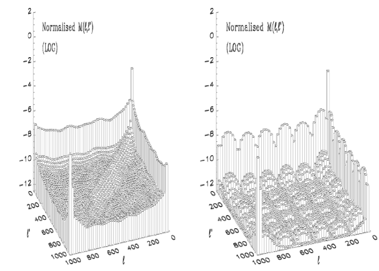
Figure 27: This figure shows the same as Fig. 26 but for $36$ and $180$ degree separation of the patches.

In Fig. 28, we did a separate $C_{\ell}$ estimation on 146 non-overlapping patches with radius $18^{\circ}$ apodised with a $15^{\circ}$ FWHM Gaussian Gabor window. The patches where uniformly distributed over the sphere and uniform noise was added to the whole map. The figure shows the average of the $146$ $C_{\ell}$ estimates. One can see that the estimate seems to be approaching the full sky power spectrum even at small multipoles.

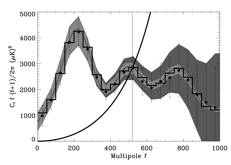
Figure 28: The average of 146 individual power spectrum estimations of 146 non-overlapping patches on the same CMB map with uniform noise added to it. The patches all had radius $18^{\circ}$ degrees apodised with a $15^{\circ}$ FWHM Gaussian Gabor window. The histogram shows the binned average of the $146$ $\tilde{C}_{\ell}$ from the different patches without noise. The dotted line is the average full sky power spectrum and the shaded areas around the binned full sky power spectrum (not plotted) show the theoretical $1\sigma$ variance with (dark) and without (bright) noise. The solid line rising from the left to the right is the noise power spectrum.

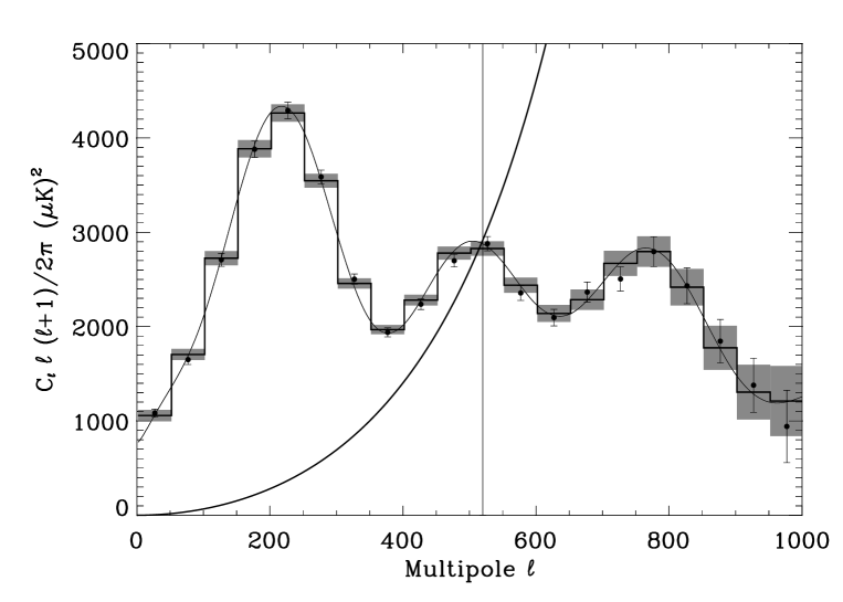
Figure 29: The result of a joint analysis of 146 patches on the same CMB map. The solid line shows the average full sky power spectrum, the histogram shows the binned full sky power spectrum and the shaded boxes show the expected $2\sigma$ deviations due to noise, cosmic and sample variance. The sizes of the shaded boxes were calculated from the formula for uniform noise (equation 32). The dots show the estimates with $2\sigma$ error bars taken from the Fisher matrix. As before the rising solid line is the noise power spectrum and the vertical line shows where $S/N=1$.

Finally we made a joint analysis of all the $146$ patches. The idea was to extend the data vector in the likelihood so that it contained the $N^{\mathrm{in}}$ $\tilde{C}_{\ell}$ from all the $146$ patches. The data vector can then be written as ${\mathbf{d}}=\{{\mathbf{d}}_{1},{\mathbf{d}}_{2},...,{\mathbf{d}}_{146}\}$ where ${\mathbf{d}}_{i}$ now denotes the whole data vector for patch number $i$. From the results above it seems to be a good approximation to assume that the correlation between $\tilde{C}_{\ell}$ from different patches is zero so that the correlation matrix will be block diagonal. Each block is then the correlation matrix for each individual patch. The log-likelihood can then simply be written as

$$L=\sum_{i=1}^{146}{\mathbf{d}}_{i}^{\mathrm{T}}{\mbox{$\textbf{{M}}$}}_{i}^{-1}{\mathbf{d}}_{i}+\sum_{i=1}^{146}\ln\det{\mbox{$\textbf{{M}}$}}_{i},$$ (35)

where ${\mbox{$\textbf{{M}}$}}_{i}$ is the correlation matrix for patch number $i$. In Fig. 29 the result of this joint analysis is shown. One can see that the full sky power spectrum is well within the two sigma error bars of the estimates.

The method of combining patches on the sky for power spectrum analysis will be developed further in a forthcoming paper.

4.2 Monte Carlo simulations of the noise correlations and extension to correlated noise

The computation of the noise correlation matrix in the general case without any approximations takes $\sqrt{N_{\mathrm{pix}}}l_{\mathrm{max}}^{2}(N^{\mathrm{in}})^{2}$ which is approximately $N_{\mathrm{pix}}^{3/2}(N^{\mathrm{in}})^{2}$ when $N_{\mathrm{pix}}$ is large ($N_{\mathrm{pix}}\approx\ell_{\mathrm{max}}^{2}$). When $N^{\mathrm{in}}$ is getting large this can be calculated quicker using Monte Carlo simulations (as was done in [Hivon et al. 2002]). Finding the $\tilde{C}_{\ell}^{\mathrm{N}}$ from one noise map takes $\mathcal{O}(N_{\mathrm{pix}}^{3/2})$ operations so using Monte Carlo simulations to find the whole noise matrix takes $\mathcal{O}(N_{\mathrm{pix}}^{3/2}N_{\mathrm{sim}})$ operation where $N_{\mathrm{sim}}$ is the number of Monte Carlo simulations needed. So when $N_{\mathrm{sim}}<<(N_{\mathrm{in}}^{2})$ it will be advantageous using MC if this gives the same result.

Also when the noise gets correlated, the analytic calculation of $\langle\tilde{a}_{\ell m}^{\mathrm{N}}\tilde{a}_{\ell^{\prime}m}^{\mathrm{N}}\rangle$ will be very expensive. In this case another method for computing $\langle\tilde{a}_{\ell m}^{\mathrm{N}}\tilde{a}_{\ell^{\prime}m}^{\mathrm{N}}\rangle$ will be necessary and Monte Carlo simulations could also prove useful. For a given noise model several noise realisations can be made and averaged to yield the noise correlation matrix and the $\langle\tilde{a}_{\ell m}^{\mathrm{N}}\tilde{a}_{\ell^{\prime}m}^{\mathrm{N}}\rangle$ term needed in the estimation process. This is of course dependent on a method for fast evaluation of maps with different realisations.

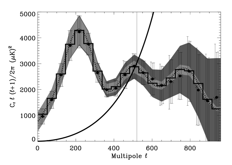
Figure 30: Same as Fig. 18 but with a different noise model. Here the average of 100 estimations is shown. The big dots in the middle of the bins show the result using analytical expressions for the noise matrices. The crosses on the left side of each big dot show the results of using noise matrices from $N_{\mathrm{sim}}=1000$ MC simulations. The crosses on the right side are for $N_{\mathrm{sim}}=20000$ noise simulations.

In figure 30, the result of $C_{\ell}$ estimation with noise matrix and $\langle a_{\ell m}^{\mathrm{N}}a_{\ell^{\prime}m}^{\mathrm{N}}\rangle$ computed with Monte Carlo is shown. Again a standard CDM power spectrum was used with a non-uniform white noise model and a $15^{\circ}$ FWHM Gaussian Gabor window. In the $C_{\ell}$ estimation $N^{\mathrm{in}}=200$ $\tilde{C}_{\ell}$ were used and $N^{\mathrm{bin}}=20$ power spectrum bins were estimated. The noise matrices were calculated using (1) the analytical expression, (2) MC with $N_{\mathrm{sim}}=20000$ and (3) MC with $N_{\mathrm{sim}}=1000$. In Fig. 31, a slice of the correlation matrices for the different cases is shown for $\ell=500$. The dashed line (case (3)) follows the solid line (case (1)) to a level of about $10^{-2}$ of the diagonal. The dotted line (case (2)) is roughly correct to about $10^{-1}$ times the value at the diagonal.

Figure 31: A slice of the noise correlation matrix at multipole $\ell=500$. The correlation matrix was evaluated using the analytical formulae (solid line), 20000 MC simulations (dashed line) and 1000 MC simulations (dotted line). The matrix is here normalised to be $1$ at the diagonal.

We did 100 estimations for each case and the average result is plotted in Fig. 30. The big dots are the results from case (1), the crosses on the right hand side are the results from (2) and the crosses on the left hand side the results from (3). The average estimates seem to be consistent, only in the highly noise dominated regime they start to deviate. For case (2), the error bars are for some multipoles higher and for some lower than the analytic case. The differences are at most $3\%$. We conclude that using this many simulations, the error bars do not increase significantly over the analytic case. For case (3) the error bars are up to $17\%$ higher (and only higher) than the analytic case. It seems that $1000$ simulations was not sufficient to keep the same accuracy of the estimates as when using analytic noise matrices. To keep the error bars close to the analytic case, it seems that a few thousand simulations are necessary.

5 Conclusion

In this paper, we propose to use the spherical harmonic transform of the sky apodised by a window function, or Gabor transform, as a fast and robust tool to estimate the CMB fluctuations power spectrum. It is known that the coupling between modes resulting from the analysis on a cut sky affects the shape of the measured pseudo power spectrum and the statistics of the $C_{\ell}$ coefficients ([Wandelt, Górski & Hivon 2000, Hivon et al. 2002] and reference therein). In the case of axisymmetric windows we can compute analytically (in about $\ell_{\mathrm{max}}^{3}$ operations) the kernel relating the cut sky power spectrum to the full sky one for a Gaussian and top-hat profile we give an analytical relation between the spectral resolution attainable and the size of the sky window. Studying windows of different sizes, we show that for windows as small as $36$ degrees in radius, the measured power spectrum is undiscernable from the true one for $\ell$ larger than about 50.

Noting that for large multipoles ($\ell\geq 100$ for windows with radius larger than $36$ degree) the statistics of the pseudo-$C_{\ell}$ coefficients measured in Monte Carlo simulations is close to Gaussian, we suggest the use of the pseudo power spectrum as input data vector in a likelihood estimation. For the first time, we show how the correlation matrix between the pseudo power spectrum coefficients obtained on an axisymmetric window of arbitrary profile can be computed rapidly for any input power spectrum, based on a recurrence relation. The computation of the correlation matrix needs a precomputation (independent of the power spectrum) of $\ell_{\mathrm{max}}N_{m}(N^{\mathrm{in}})^{2}$ operations and each calculation of the correlation matrix with a given power spectrum takes $(N^{\mathrm{in}})^{2}(N^{\mathrm{bin}})^{2}$ operations, where $N^{\mathrm{in}}$ is the number of input pseudo-$C_{\ell}$ coefficients used, $N^{\mathrm{bin}}$ is the number of estimated $C_{\ell}$ bins and $N_{m}$ is a window dependent factor ($N_{m}\approx 200$ for a Gaussian window and $N_{m}\approx 400$ for a top-hat window). The noise correlation matrix can also be computed by recurrence. For axisymmetric noise this is very quick ($N_{\mathrm{pix}}\ell_{\mathrm{max}}$ operations). For general non-uniform noise this takes some more time (between $(N^{\mathrm{in}})^{2}\sqrt{N_{\mathrm{pix}}}\ell_{\mathrm{max}}$ and $(N_{\mathrm{in}})^{2}\sqrt{N_{\mathrm{pix}}}\ell_{\mathrm{max}}^{2}$ operations dependent on the window profile and number of approximations). For a Gaussian window with a sharply varying noise profile and a patch of sky similar in size to the one observed by BOOMERANG (about $2\%$ of the sky) it takes about a day on one single $500\mathrm{MHz}$ processor. This is the computationally heaviest part of the method but this has to be done only once. The inversion of the correlation matrix, which is the leading problem when doing likelihood analysis, is now overcome, as the size of the correlation matrix is so small that inversion is feasible. In the standard likelihood approach, the correlation matrix has dimensions $N_{\mathrm{pix}}\times N_{\mathrm{pix}}$ which needs $N_{\mathrm{pix}}^{3}$ operations to be inverted. In our approach, the size of the correlation matrix is $N^{\mathrm{in}}\times N^{\mathrm{in}}$ which in our example $N^{\mathrm{in}}=200$ is inverted in a few seconds.

By doing Monte Carlo simulations of different experimental settings, we shown that the likelihood estimator is unbiased. The error bars were found using the inverse Fisher matrix and compared to the error bars obtained from Monte Carlo. There was an excellent agreement between the two sets of error bars. In [Hivon et al. 2002] it was shown that using a Gaussian apodisation suppresses the signal such that the error bars on the estimated power spectrum becomes larger. In this paper we have shown that using a different window than the top-hat window can be important for increasing the signal-to-noise ratio in data with non-uniform noise. We applied a Gaussian window to an observed disc which had the noise level increasing from the centre of the disc and outwards similar to what one can expect around the ecliptic poles in scanning strategies like the ones of MAP and Planck. In this case the Gaussian window has a high value in the centre where signal-to-noise per pixel is high and a low value close to the more noise dominated edges. We shown that for this noise profile using a Gaussian window increased the signal-to-noise ratio significantly over the top-hat window, showing that adapting the window to downweight noisy pixels gives better performance than a simple uniform weighting.

Finally two extensions of the power spectrum estimation method were discussed. First it was shown that for observed areas on the sky which are not axisymmetric, one can cover the area by several axisymmetric patches and make a joint analysis of the pseudo power spectrum coefficients from all the patches. Each of the patches can have a different window in order to optimise signal-to-noise in each patch. This method will be extended in a forthcoming paper where we will discuss the use of the method for analysing MAP and Planck data sets. We also shown that the calculation of the noise correlation matrix can be quicker by Monte Carlo simulations if the number of pixels in the observed area is huge (about $10^{6}$ pixels but dependent on the window shape). This may also be used in the case of correlated noise. We shown that a few thousand simulations are necessary to get the same accuracy in the power spectrum estimates as when using the analytic formula for the noise correlation matrix.

In [Hansen & Górski 2002] we show that the power spectrum estimation method presented in this paper can easily be extended to polarisation. By extending the data vector in the likelihood to have also the pseudo-$C_{\ell}$ from polarisation, one can in a similar way estimate for the temperature and polarisation power spectra jointly.

Appendix A Rotation Matrices

A spherical function $T({\mathbf{\hat{n}}})$ is rotated by the operator $\hat{D}(\alpha\beta\gamma)$ where $\alpha\beta\gamma$ are the three Euler angles for rotations (See T.Risbo 1996) and the inverse rotation is $\hat{D}(-\gamma-\beta-\alpha)$. For the spherical harmonic functions, this operator takes the form,

$$Y_{\ell m}({\mathbf{\hat{n}}}^{\prime})=\sum_{m^{\prime}=-\ell}^{\ell}D_{m^{\prime}m}^{\ell}(\alpha\beta\gamma)Y_{\ell m^{\prime}}({\mathbf{\hat{n}}}),$$ (36)

where $D_{m^{\prime}m}^{\ell}$ has the form

$$D_{m^{\prime}m}^{\ell}(\alpha\beta\gamma)=\mathrm{e}^{\mathrm{i}m^{\prime}\alpha}d_{m^{\prime}m}^{\ell}(\beta)\mathrm{e}^{\mathrm{i}m\gamma}.$$ (37)

Here $d_{m^{\prime}m}^{\ell}(\beta)$ is a real coefficient with the following property:

$$d_{m^{\prime}m}^{\ell}(\beta)=d_{mm^{\prime}}^{\ell}(-\beta).$$ (38)

The D-functions also have the following property:

$$D_{m^{\prime}m}^{\ell}(\alpha\beta\gamma)=\sum_{m^{\prime\prime}}D_{m^{\prime}m^{\prime\prime}}^{\ell}(\alpha_{2}\beta_{2}\gamma_{2})D_{m^{\prime\prime}m}^{\ell}(\alpha_{1}\beta_{1}\gamma_{1}),$$ (39)

where $(\alpha\beta\gamma)$ is the result of the two consecutive rotations $(\alpha_{1}\beta_{1}\gamma_{1})$ and $(\alpha_{2}\beta_{2}\gamma_{2})$.

The complex conjugate of the rotation matrices can be written as

$$D^{\ell*}_{mm^{\prime}}=(-1)^{m+m^{\prime}}D^{\ell}_{(-m)(-m^{\prime})}.$$ (40)

Appendix B Some Wigner Symbol Relations

Throughout the paper, the Wigner 3j Symbols will be used frequently. Here are some relations for these symbols, which are used. The orthogonality relation is,

$$\sum_{mm^{\prime}}{\left(\begin{array}[]{ccc}\ell&\ell^{\prime}&\ell^{\prime\prime}\\ m&m^{\prime}&m^{\prime\prime}\\ \end{array}\right)}{\left(\begin{array}[]{ccc}\ell&\ell^{\prime}&L^{\prime\prime}\\ m&m^{\prime}&M^{\prime\prime}\\ \end{array}\right)}=(2\ell^{\prime\prime}+1)^{-1}\delta_{\ell^{\prime\prime}L^{\prime\prime}}\delta_{m^{\prime\prime}M^{\prime\prime}}.$$ (41)

The Wigner 3j Symbols can be represented as an integral of rotation matrices (see Appendix(A)),

$$\frac{1}{8\pi^{2}}\int d\cos\theta d\phi d\gamma D_{m_{1}m^{\prime}_{1}}^{\ell}D_{m_{2}m^{\prime}_{2}}^{\ell^{\prime}}D_{m_{3}m^{\prime}_{3}}^{\ell^{\prime\prime}}={\left(\begin{array}[]{ccc}\ell&\ell^{\prime}&\ell^{\prime\prime}\\ m_{1}&m_{2}&m_{3}\\ \end{array}\right)}{\left(\begin{array}[]{ccc}\ell&\ell^{\prime}&\ell^{\prime\prime}\\ m^{\prime}_{1}&m^{\prime}_{2}&m^{\prime}_{3}\\ \end{array}\right)}.$$ (42)

This expression can be reduced to,

$$\int d{\mathbf{\hat{n}}}Y_{\ell m}({\mathbf{\hat{n}}})Y_{\ell^{\prime}m^{\prime}}({\mathbf{\hat{n}}})Y_{\ell^{\prime\prime}m^{\prime\prime}}({\mathbf{\hat{n}}})=\sqrt{\frac{(2\ell+1)(2\ell^{\prime}+1)(2\ell^{\prime\prime}+1)}{4\pi}}{\left(\begin{array}[]{ccc}\ell&\ell^{\prime}&\ell^{\prime\prime}\\ m&m^{\prime}&m^{\prime\prime}\\ \end{array}\right)}{\left(\begin{array}[]{ccc}\ell&\ell^{\prime}&\ell^{\prime\prime}\\ 0&0&0\\ \end{array}\right)}.$$ (43)

Appendix C Recurrence Relation

It is important for the precalculations to the likelihood analysis that the calculation of $h(\ell,\ell^{\prime},m)$ is fast. For this reason a recurrence relation for $h(\ell,\ell^{\prime},m)$ would be helpful. To speed up the calculation of the noise correlation matrix for non-axisymmetric noise, it would also help if one had a more general recurrence relation for $h(\ell,\ell^{\prime},m,m^{\prime})$. We will now show how to find such a recurrence for these objects which we now call $A_{\ell^{\prime}\ell}^{m^{\prime}m}$ to simplify notation (and for the notation to comply with [Wandelt, Górski & Hivon 2000]). The definition is again,

$$A_{\ell^{\prime}\ell}^{m^{\prime}m}=\int_{a}^{b}G({\mathbf{\hat{n}}})Y^{*}_{\ell m}({\mathbf{\hat{n}}})Y_{\ell^{\prime}m^{\prime}}({\mathbf{\hat{n}}})d{\mathbf{\hat{n}}},$$ (44)

where $G({\mathbf{\hat{n}}})=G(\theta,\phi)$ is a general function and $Y_{\ell m}$ are the spherical harmonics which can be factorised into one part dependent on $\theta$ and one dependent on $\phi$ in the following way,

$$Y_{\ell m}(\theta,\phi)=\lambda_{\ell m}(\cos{\theta})\mathrm{e}^{-\mathrm{i}\phi m}.$$ (45)

Now writing,

$$A_{\ell^{\prime}\ell}^{m^{\prime}m} = \int d\cos\theta\lambda_{\ell m}(\cos\theta)\lambda_{\ell^{\prime}m^{\prime}}(\cos\theta)\int d\phi\mathrm{e}^{-\mathrm{i}\phi(m-m^{\prime})}G(\theta,\phi)$$ (46)

$$\equiv \int d\cos\theta\lambda_{\ell m}(\cos\theta)\lambda_{\ell^{\prime}m^{\prime}}(\cos\theta)F_{m^{\prime}m}(\theta),$$ (47)

where $F_{m^{\prime}m}(\theta)$ is simply the Fourier transform of the window at each $\theta$. The quantities $A_{\ell^{\prime}\ell}^{m^{\prime}m}$ and $F_{m^{\prime}m}(\theta)$ are in general complex quantities obeying,

$$A_{\ell^{\prime}\ell}^{m^{\prime}m}=(A_{\ell\ell^{\prime}}^{mm^{\prime}})^{*}\ \ \ F_{m^{\prime}m}(\theta)=(F_{mm^{\prime}}(\theta))^{*}$$ (48)

The $A_{\ell^{\prime}\ell}^{m^{\prime}m}$ can be expressed as

$$A_{\ell^{\prime}\ell}^{m^{\prime}m}=\frac{\sqrt{(2\ell^{\prime}+1)(2\ell+1)}}{2}\sqrt{\frac{(\ell^{\prime}-m^{\prime})!(\ell-m)!}{(\ell^{\prime}+m^{\prime})!(\ell+m)!}}I_{\ell^{\prime}\ell}^{m^{\prime}m},$$ (49)

where $I_{\ell^{\prime}\ell}^{m^{\prime}m}$ is defined as:

$$I_{\ell^{\prime}\ell}^{m^{\prime}m}=\int_{a}^{b}F_{m^{\prime}m}(x)P_{\ell}^{m}(x)P_{\ell^{\prime}}^{m^{\prime}}(x)dx.$$ (50)

The following relation for the Legendre Polynomials will be used:

$$xP_{\ell}^{m}=\frac{\ell-m+1}{2\ell+1}P_{\ell+1}^{m}+\frac{\ell+m}{2\ell+1}P_{\ell-1}^{m}$$ (51)

We now define the object $X_{\ell^{\prime}\ell}^{m^{\prime}m}$ as

$$X_{\ell^{\prime}\ell}^{m^{\prime}m}=\int_{a}^{b}F_{m^{\prime}m}(x)xP_{\ell}^{m}P_{\ell^{\prime}}^{m^{\prime}}dx$$ (52)

Using relation (51) in this definition, one gets,

$$X_{\ell^{\prime}\ell}^{m^{\prime}m}=\frac{\ell-m+1}{2\ell+1}I_{\ell^{\prime}(\ell+1)}^{m^{\prime}m}+\frac{\ell+m}{2\ell+1}I_{\ell^{\prime}(\ell-1)}^{m^{\prime}m}$$ (53)

One can also exchange $(\ell,\ell^{\prime})$ and $(m,m^{\prime})$ to get

$$X_{\ell\ell^{\prime}}^{mm^{\prime}}=\frac{\ell^{\prime}-m^{\prime}+1}{2\ell^{\prime}+1}I_{\ell(\ell^{\prime}+1)}^{mm^{\prime}}+\frac{\ell^{\prime}+m^{\prime}}{2\ell^{\prime}+1}I_{\ell(\ell^{\prime}-1)}^{mm^{\prime}}$$ (54)

Taking the complex conjugate of the first expression and subtracting the last, one has

$$(X_{\ell^{\prime}\ell}^{m^{\prime}m})^{*}-X_{\ell\ell^{\prime}}^{mm^{\prime}}=0 = \frac{\ell-m+1}{2\ell+1}(I_{\ell^{\prime}(\ell+1)}^{m^{\prime}m})^{*}+\frac{\ell+m}{2\ell+1}(I_{\ell^{\prime}(\ell-1)}^{m^{\prime}m})^{*}$$ (56)

$$-\frac{\ell^{\prime}-m+1}{2\ell^{\prime}+1}I_{\ell(\ell^{\prime}+1)}^{mm^{\prime}}-\frac{\ell^{\prime}+m}{2\ell^{\prime}+1}I_{\ell(\ell^{\prime}-1)}^{mm^{\prime}}$$

Then setting $\ell^{\prime}=\ell^{\prime}-1$ one gets:

$$I_{\ell^{\prime}\ell}^{m^{\prime}m}=\frac{2\ell^{\prime}-1}{\ell^{\prime}-m^{\prime}}\left(\frac{\ell-m+1}{2\ell+1}I_{(\ell^{\prime}-1)(\ell+1)}^{m^{\prime}m}+\frac{\ell+m}{2\ell+1}I_{(\ell^{\prime}-1)(\ell-1)}^{m^{\prime}m}-\frac{\ell^{\prime}+m-1}{2\ell^{\prime}-1}I_{(\ell^{\prime}-2)\ell}^{m^{\prime}m}\right)$$ (57)

Using equation (49), one can express this as

$$A_{\ell^{\prime}\ell}^{m^{\prime}m} = \frac{1}{\sqrt{{\ell^{\prime}}^{2}-m^{\prime 2}}}\biggl{(}\sqrt{\frac{(4{\ell^{\prime}}^{2}-1)((\ell+1)^{2}-m^{2})}{(2\ell+1)(2\ell+3)}}A_{(\ell^{\prime}-1)(\ell+1)}^{m^{\prime}m}$$

$$+\sqrt{\frac{(4{\ell^{\prime}}^{2}-1)(\ell^{2}-m^{2})}{4\ell^{2}-1}}A_{(\ell^{\prime}-1)(\ell-1)}^{m^{\prime}m}-\sqrt{\frac{(2\ell^{\prime}+1)((\ell^{\prime}-1)^{2}-m^{\prime 2})}{2\ell^{\prime}-3}}A_{(\ell^{\prime}-2)\ell}^{m^{\prime}m}\biggl{)},$$

which is the final recurrence relation. The $A_{m^{\prime}\ell}^{m^{\prime}m}$ elements must be provided before the recurrence is started. Then for each $(m,m^{\prime})$, set $\ell^{\prime}=m^{\prime}+1$ and let $\ell$ go from $\ell^{\prime}$ and upwards, then set $\ell^{\prime}=m^{\prime}+2$ and again let $\ell$ go from $\ell^{\prime}$ and upwards. Continue to the desired size of $\ell^{\prime}$. Note that, in order to get all objects up to $A_{\ell_{\mathrm{max}}\ell_{\mathrm{max}}}^{m^{\prime}m}$ one always needs to go up to $\ell=2\ell_{\mathrm{max}}$ during recursion. This is because of the $A_{(\ell^{\prime}-1)(\ell+1)}^{m^{\prime}m}$ term which demands an object indexed $(\ell+1)$ in the previous $\ell^{\prime}$ row.
To start the recurrence, one can precomputed the $A^{m^{\prime}m}_{m^{\prime}\ell}$ factors fast and easily using FFT and a sum over rings on the grid. F.ex. for the HEALPix grid, we did it the following way,

$$A_{m^{\prime}\ell}^{m^{\prime}m}=\sum_{r}\lambda^{r}_{m^{\prime}m^{\prime}}\lambda^{r}_{\ell m}\sum_{j=0}^{N_{r}-1}\mathrm{e}^{-2\pi ij/N_{r}(m-m^{\prime})}G_{rj},$$ (59)

where the last part is the Fourier transform of the Gabor window, calculated by FFT, $r$ is ring number on the grid and $j$ is azimuthal position on each ring. Ring $r$ has $N_{r}$ pixels.

It turns out that the recurrence can be numerically unstable dependent on the window and multipole, and in order to avoid problems we (using double precision numbers) restart the recurrence with a new set of precomputed $A^{m^{\prime}m}_{\ell^{\prime}\ell}$ for every 50th $\ell^{\prime}$ row. However for most windows and multipoles that we tested the recurrence can run for hundreds of $\ell$-rows without problems.

Appendix D Rotational Invariance

It was shown that the average $\langle\tilde{C}_{\ell}\rangle$ is invariant under rotations of the Gabor window. We will now show that the non-averaged $\tilde{C}_{\ell}$ are rotationally invariant under any rotation of the sky AND Gabor window by the same angle. This fact justifies that we can always put the window on the north pole since this simplifies the calculations. In the following we will use the rotation matrices $D^{\ell}_{mm^{\prime}}$ described in Appendix (A). Consider a rotation of the sky and window by the angles $(-\gamma-\beta-\alpha)$. Then the $\tilde{a}_{\ell m}$ becomes,

$$\tilde{a}_{\ell m}^{\mathrm{rot}}=\int d{\mathbf{\hat{n}}}[\hat{D}(-\gamma-\beta-\alpha)T({\mathbf{\hat{n}}})G({\mathbf{\hat{n}}})]Y^{*}_{\ell m}({\mathbf{\hat{n}}}).$$ (60)

If one makes the inverse rotation of the integration angle ${\mathbf{\hat{n}}}$, one can write this as

$$\tilde{a}_{\ell m}^{\mathrm{rot}}=\int d{\mathbf{\hat{n}}}T({\mathbf{\hat{n}}})G({\mathbf{\hat{n}}})[\hat{D}^{*}(\alpha\beta\gamma)Y^{*}_{\ell m}({\mathbf{\hat{n}}})],$$ (61)

which is just

$$\tilde{a}_{\ell m}^{\mathrm{rot}}=\sum_{m^{\prime}}D_{m^{\prime}m}^{\ell*}(\alpha\beta\gamma)\int d{\mathbf{\hat{n}}}T({\mathbf{\hat{n}}})G({\mathbf{\hat{n}}})Y^{*}_{\ell m^{\prime}}({\mathbf{\hat{n}}}).$$ (62)

One can identify the last integral as the normal $\tilde{a}_{\ell m}$.

$$\tilde{a}_{\ell m}^{\mathrm{rot}}=\sum_{m^{\prime}}D_{m^{\prime}m}^{\ell*}(\alpha\beta\gamma)\tilde{a}_{\ell m}.$$ (63)

So the $\tilde{a}_{\ell m}$ are NOT rotationally invariant. Rotation mixes $m$-modes for a given $\ell$-value.

Now to the $\tilde{C}_{l}$. One has that

$$\tilde{C}_{\ell}^{\mathrm{rot}} = \frac{1}{2\ell+1}\sum_{m}a^{\mathrm{rot}}_{\ell m}a^{\mathrm{rot*}}_{\ell m}$$ (64)

$$= \frac{1}{2\ell+1}\sum_{m}\sum_{m^{\prime}}\sum_{m^{\prime\prime}}D_{m^{\prime}m}^{\ell}(\alpha\beta\gamma)D_{m^{\prime\prime}m}^{\ell*}(\alpha\beta\gamma)\tilde{a}_{\ell m^{\prime}}\tilde{a}_{\ell m^{\prime\prime}}^{*}$$ (65)

$$= \frac{1}{2\ell+1}\sum_{m^{\prime}m^{\prime\prime}}\tilde{a}_{\ell m^{\prime}}\tilde{a}_{\ell m^{\prime\prime}}^{*}\sum_{m}D_{m^{\prime}m}^{\ell}(\alpha\beta\gamma)D_{m^{\prime\prime}m}^{\ell*}(\alpha\beta\gamma).$$ (66)

Using the properties given in Appendix (A), one can write the last D-function on the last line as,

$$\hat{D}_{m^{\prime\prime}m}^{\ell*}(\alpha\beta\gamma) = D_{m^{\prime\prime}m}^{\ell}(-\alpha\beta-\gamma)$$ (67)

$$= \mathrm{e}^{-\mathrm{i}m^{\prime\prime}\alpha}d_{m^{\prime\prime}m}^{\ell}(\beta)\mathrm{e}^{-\mathrm{i}m\gamma}$$ (68)

$$= \mathrm{e}^{-\mathrm{i}m^{\prime\prime}\alpha}d_{mm^{\prime\prime}}^{\ell}(-\beta)\mathrm{e}^{-\mathrm{i}m\gamma}$$ (69)

$$= D_{mm^{\prime\prime}}^{\ell}(-\gamma-\beta-\alpha).$$ (70)

Knowing that $(-\gamma-\beta-\alpha)$ is the inverse rotation of $(\alpha\beta\gamma)$ one can write,

$$\sum_{m}D_{m^{\prime}m}^{\ell}(\alpha\beta\gamma)D_{m^{\prime\prime}m}^{\ell*}(\alpha\beta\gamma) = \sum_{m}D_{m^{\prime}m}^{\ell}(\alpha\beta\gamma)D_{mm^{\prime\prime}}^{\ell}(-\gamma-\beta-\alpha)$$ (71)

$$= D_{m^{\prime}m^{\prime\prime}}^{\ell}(000)=\delta_{m^{\prime}m^{\prime\prime}}$$ (72)

So one gets,

$$\tilde{C}_{\ell}^{\mathrm{rot}}=\tilde{C}_{\ell}.$$ (73)

Appendix E The Correlation Matrix

To do fast likelihood analysis with $\tilde{C}_{\ell}$ one needs to be able to calculate $\langle\tilde{C}_{\ell}\rangle$ and the correlations $\langle\tilde{C}_{\ell}\tilde{C}_{\ell^{\prime}}\rangle$ fast. Calculating the average $\langle\tilde{C}_{\ell}\rangle$ by formula (16) using the analytic expression (17) for the kernel is not very fast. It turns out that a faster way of evaluating the kernel is by using direct integration (summation on the pixelised sphere) and then, as shown in Appendix (C), recurrence. By means of an integral, one can then write the $\tilde{a}_{\ell m}$ as (now assuming that ${\mathbf{\hat{n}}}_{0}$ is on the north pole),

$$\tilde{a}_{\ell m} = \sum_{\ell^{\prime}m^{\prime}}a_{\ell^{\prime}m^{\prime}}\int G({\mathbf{\hat{n}}})Y^{*}_{\ell m}({\mathbf{\hat{n}}})Y_{\ell^{\prime}m^{\prime}}({\mathbf{\hat{n}}})d{\mathbf{\hat{n}}}$$ (74)

$$= \sum_{\ell^{\prime}m^{\prime}}a_{\ell^{\prime}m^{\prime}}\int G(\theta)\lambda_{\ell m}(\theta)\lambda_{\ell^{\prime}m^{\prime}}(\theta)d\cos{\theta}\underbrace{\int\mathrm{e}^{-\mathrm{i}\phi(m-m^{\prime})}d\phi}_{2\pi\delta_{mm^{\prime}}}$$

$$= \sum_{\ell^{\prime}}a_{\ell^{\prime}m}2\pi\int G(\theta)\lambda_{\ell m}(\theta)\lambda_{\ell^{\prime}m}(\theta)d\cos{\theta}$$

$$\equiv \sum_{\ell^{\prime}}a_{\ell^{\prime}m}h(\ell,\ell^{\prime},m),$$

where the last line defines $h(\ell,\ell^{\prime},m)$ and $\lambda_{\ell m}(\theta)$ is given by,

$$Y_{\ell m}(\theta,\phi)=\lambda_{\ell m}(\theta)\mathrm{e}^{-\mathrm{i}\phi m}.$$ (75)

Using this form, one gets,

$$\langle\tilde{C}_{\ell}\rangle=\frac{1}{2\ell+1}\sum_{\ell^{\prime}}C_{\ell^{\prime}}\sum_{m}h^{2}(\ell,\ell^{\prime},m).$$ (76)

To obtain this expression, ${\mathbf{\hat{n}}}_{0}$ was on the north pole, but as was shown, the $\langle\tilde{C}_{\ell}\rangle$s are rotationally invariant, that is $\langle\tilde{C}_{\ell}\rangle$ remains the same if one rotates the Gabor window so that it is centred on the north pole.

When using real CMB data, the observed temperature map is always pixelised. So an integral over the sphere has to be replaced by a sum over pixels. In this case, the formula for $h(\ell,\ell^{\prime},m)$ has to be replaced by

$$h(\ell,\ell^{\prime},m)=\sum_{j}G_{j}\lambda_{\ell m}^{j}\lambda_{\ell^{\prime}m}^{j}\Delta_{j},$$ (77)

where the index $j$ is the pixel number replacing the angle $\theta$ and $\Delta_{j}$ is the area of pixel $j$. Using a pixelisation scheme like HEALPix [Górski, Hivon and Wandelt 1998] which has a structure of azimuthal rings going from the north to the south pole with $N_{r}$ pixels in ring $r$ and equal area for each pixel $\Delta_{j}=\Delta$ this can be written as

$$h(\ell,\ell^{\prime},m) = \Delta\sum_{r}\sum_{p=0}^{N_{r}-1}G_{r}\lambda_{\ell m}^{r}\lambda_{\ell^{\prime}m}^{r},$$ (78)

$$= \Delta\sum_{r}N_{r}G_{r}\lambda_{\ell m}^{r}\lambda_{\ell^{\prime}m}^{r}.$$

Here the sum over pixels is split into a sum over rings $r$ and a sum over the pixels in each ring $p$. The first sum goes over all rings which have $\theta<\theta_{\mathrm{C}}$.

Using this expression for the $\tilde{a}_{\ell m}$ one can now find the correlation matrix

$$\langle\tilde{C}_{\ell}\tilde{C}_{\ell^{\prime}}\rangle=\sum_{mm^{\prime}}\frac{\langle\tilde{a}_{\ell m}^{*}\tilde{a}_{\ell m}\tilde{a}_{\ell^{\prime}m^{\prime}}^{*}\tilde{a}_{\ell^{\prime}m^{\prime}}\rangle}{(2\ell+1)(2\ell^{\prime}+1)}.$$ (79)

In this expression one can use relation (74) to get,

$$\langle\tilde{C}_{\ell}\tilde{C}_{\ell^{\prime}}\rangle = \frac{1}{(2\ell+1)(2\ell^{\prime}+1)}\sum_{mm^{\prime}}\sum_{LL^{\prime}KK^{\prime}}\langle a_{Lm}^{*}a_{L^{\prime}m}a_{Km^{\prime}}^{*}a_{K^{\prime}m^{\prime}}\rangle$$ (81)

$$\times h(\ell,L,m)h(\ell,L^{\prime},m)h(\ell^{\prime},K,m^{\prime})h(\ell^{\prime},K^{\prime},m^{\prime})$$

$$= \frac{1}{(2\ell+1)(2\ell^{\prime}+1)}$$ (82)

$$\times \sum_{mm^{\prime}}\sum_{LL^{\prime}KK^{\prime}}[\langle a_{Lm}^{*}a_{L^{\prime}m}\rangle\langle a_{Km^{\prime}}^{*}a_{K^{\prime}m^{\prime}}\rangle$$ (85)

$$+\langle a_{Lm}^{*}a_{Km^{\prime}}^{*}\rangle\langle a_{L^{\prime}m}a_{K^{\prime}m^{\prime}}\rangle$$

$$+\langle a_{Lm}^{*}a_{K^{\prime}m^{\prime}}\rangle\langle a_{L^{\prime}m}a_{Km^{\prime}}^{*}\rangle]$$

$$\times h(\ell,L,m)h(\ell,L^{\prime},m)h(\ell^{\prime},K,m^{\prime})h(\ell^{\prime},K^{\prime},m^{\prime}).$$ (86)

Clearly the first term is just the product $\langle\tilde{C}_{\ell}\rangle\langle\tilde{C}_{\ell^{\prime}}\rangle$, and the two last terms are equal (using $a_{Km^{\prime}}^{*}=a_{Km^{\prime}}(-1)^{m^{\prime}}$ and $a_{K^{\prime}m^{\prime}}=(-1)^{m^{\prime}}a^{*}_{K^{\prime}m^{\prime}}$) so one gets,

$$M_{ij}=\frac{2}{(2\ell+1)(2\ell^{\prime}+1)}\sum_{m}\left(\sum_{L}C_{L}h(\ell_{i},L,m)h(\ell_{j},L,m)\right)^{2}.$$ (87)

This is one of the main results of this paper since the formula allows one to analytically calculate the correlation matrix needed for likelihood analysis. Another main result is the recurrence deduced in appendix (C) which allows fast evaluation of the $h(\ell,\ell^{\prime},m)$ functions and thereby this correlation matrix.

By using the binning of the power spectrum described in equation (28), the correlation matrix can be calculated faster if it is written as

$$M^{\mathrm{S}}_{ij}=\sum_{b}\sum_{b^{\prime}}D_{b}D_{b^{\prime}}\chi(b,b^{\prime},i,j),$$ (88)

where $\chi(b,b^{\prime},i,j)$ is given as,

$$\chi(b,b^{\prime},i,j) \equiv \frac{2}{(2\ell_{i}+1)(2\ell_{j}+1)}$$ (89)

$$\times \sum_{m}\left(\sum_{l\epsilon b}B_{\ell}^{2}\ell(\ell+1)h(\ell,\ell_{i},m)h(\ell,\ell_{j},m)\right)$$

$$\times\left(\sum_{l\epsilon b^{\prime}}B_{\ell}^{2}\ell(\ell+1)h(\ell,\ell_{i},m)h(\ell,\ell_{j},m)\right),$$

which is precomputed. The sums over $\ell$ here go over the $\ell$ values in each specific bin $b$. One sees that computing the likelihood takes of the order $(N^{\mathrm{bin}})^{2}(N^{\mathrm{in}})^{2}$ operations whereas the precomputation of the factor $\chi(b,b^{\prime},i,j)$ goes as $\ell_{\mathrm{max}}(N^{\mathrm{in}})^{2}N_{m}$ where $N_{m}$ is the number of $m$ values used. Note that the multipole coefficients of the beam $B_{\ell}$ are also included. The reason is that the input data is always affected by the beam and this is corrected for by using the beam convolved full sky power spectrum $C_{\ell}B_{\ell}^{2}$.

The sum over $m$ in the expressions for the covariance matrix and $\langle\tilde{C}_{\ell}\rangle$ can be limited. The $h$-functions are rapidly decreasing for increasing $m$ for Gaussian and top-hat windows. For Gaussian Gabor windows it seems that one can cut the sums over $m$ at $N_{m}=200$ to high accuracy. For top-hat windows, the sum should be extended to $N_{m}=400$.

Appendix F Including White Noise

In this appendix the total $\langle\tilde{C}_{\ell}\rangle$ and the correlation matrix including contributions from white noise is found analytically. We assume that each pixel $j$ has a noise temperature denoted by $n_{j}$, with the following properties,

$$\langle n_{j}\rangle=0,\ \ \ \langle n_{j}n_{j^{\prime}}\rangle=\delta_{jj^{\prime}}\sigma^{2}_{j},$$ (90)

where $\sigma_{j}$ is the noise variance in pixel $j$. Then one has the following expressions for the $a_{\ell m}$ and $C_{l}$ (we use superscript $N$ for noise quantities),

$$a_{\ell m}^{\mathrm{N}} = \sum_{j}n_{j}Y^{j*}_{\ell m}\Delta_{j}$$ (91)

$$\langle a_{\ell m}^{\mathrm{N}}{a_{\ell^{\prime}m^{\prime}}^{\mathrm{N}}}^{*}\rangle = \sum_{jj^{\prime}}\langle n_{j}n_{j^{\prime}}\rangle Y_{\ell m}^{j}{Y_{\ell m}^{j^{\prime}}}^{*}\Delta_{j}\Delta_{j^{\prime}}=\sum_{j}\sigma_{j}^{2}Y_{\ell m}^{j}{Y_{\ell^{\prime}m^{\prime}}^{j}}^{*}\Delta_{j}^{2}$$ (92)

$$\langle C_{\ell}^{\mathrm{N}}\rangle = \frac{1}{2\ell+1}\sum_{m}\langle a_{\ell m}^{\mathrm{N}}{a_{\ell m}^{\mathrm{N}}}^{*}\rangle=\frac{1}{4\pi}\sum_{j}\sigma_{j}^{2}\Delta_{j}^{2}.$$ (93)

Here $Y_{\ell m}^{j}$ is the Spherical Harmonic of the pixel centre of pixel $j$. For the windowed coefficients, one gets similarly,

$$\tilde{a}_{\ell m}^{\mathrm{N}} = \sum_{j}G_{j}n_{j}\Delta_{j}Y_{\ell m}^{j*}$$ (94)

$$\tilde{C}_{\ell}^{\mathrm{N}} = \frac{1}{4\pi}\sum_{j}\sigma_{j}^{2}G_{j}^{2}\Delta_{j}^{2}$$ (95)

The next step is to find the noise correlation matrix,

$$\langle\tilde{C}_{\ell}^{\mathrm{N}}\tilde{C}_{\ell^{\prime}}^{\mathrm{N}}\rangle = \frac{1}{(2\ell+1)(2\ell^{\prime}+1)}\sum_{mm^{\prime}}\sum_{jj^{\prime}kk^{\prime}}\Delta_{j}\Delta_{j^{\prime}}\Delta_{k}\Delta_{k^{\prime}}$$ (96)

$$\times \langle n_{j}n_{j^{\prime}}n_{k}n_{k^{\prime}}\rangle G_{j}G_{j^{\prime}}G_{k}G_{k^{\prime}}Y_{\ell m}^{j}Y_{\ell m}^{j^{\prime}}Y_{\ell^{\prime}m^{\prime}}^{k}Y_{\ell^{\prime}m^{\prime}}^{k^{\prime}}$$ (97)

$$= \langle C_{\ell}^{\mathrm{N}}\rangle\langle C_{\ell^{\prime}}^{\mathrm{N}}\rangle+M_{\ell\ell^{\prime}}^{\mathrm{N}},$$ (98)

where $M_{\ell\ell^{\prime}}^{\mathrm{N}}$ can be written as,

$$M_{\ell\ell^{\prime}}^{\mathrm{N}}=\frac{2}{(2\ell+1)(2\ell^{\prime}+1)}\sum_{mm^{\prime}}\left(\sum_{j}\Delta_{j}^{2}G_{j}^{2}\sigma_{j}^{2}{Y_{\ell m}^{j}Y_{\ell^{\prime}m^{\prime}}^{j}}^{*}\right)^{2}\\$$ (99)

For pixelisation schemes like HEALPix, the expression can be evaluated fast using FFT. This is apparent when one writes the sum over pixels as a double sum over rings and pixels per ring.

$$\sum_{j}\Delta_{j}^{2}G_{j}^{2}\sigma_{j}^{2}{Y_{\ell m}^{j}Y_{\ell^{\prime}m^{\prime}}^{j}}^{*}=\sum_{r}\Lambda_{\ell m}^{r}\Lambda_{\ell^{\prime}m^{\prime}}^{r}\sum_{p=0}^{N_{r}-1}\mathrm{e}^{-\mathrm{i}\phi_{p}(m-m^{\prime})}\Delta^{2}G_{r}^{2}\sigma_{r,p}^{2}.$$ (100)

In the case of an axisymmetric noise model, this expression becomes even easier which is apparent writing this as

$$\sum_{r}\Lambda_{\ell m}^{r}\Lambda_{\ell^{\prime}m^{\prime}}^{r}\Delta^{2}G_{r}^{2}\sigma_{r}^{2}\underbrace{\sum_{p=0}^{N_{r}-1}\mathrm{e}^{-\mathrm{i}\phi_{p}(m-m^{\prime})}}_{N_{r}\delta_{mm^{\prime}}}=\Delta\sum_{r}\Lambda_{\ell m}^{r}\Lambda_{\ell^{\prime}m}^{r}\underbrace{\Delta G_{r}^{2}\sigma_{r}^{2}}_{G^{\prime}_{r}}\equiv h^{\prime}(\ell,\ell^{\prime},m).$$ (101)

The sum is equivalent to the previous expression for $h(\ell,\ell^{\prime},m)$ (equation 78) with a new window $G^{\prime}_{r}$. This motivates the definition of $h(\ell,\ell^{\prime},m,m^{\prime})$ such that

$$M_{\ell\ell^{\prime}}^{\mathrm{N}}=\frac{2}{(2\ell+1)(2\ell^{\prime}+1)}\sum_{mm^{\prime}}h^{\prime 2}(\ell,\ell^{\prime},m,m^{\prime}),$$ (102)

where

$$h^{\prime}(\ell,\ell^{\prime},m,m^{\prime})\equiv\Delta\sum_{j}G^{\prime}_{j}Y_{\ell m}^{j}Y_{\ell^{\prime}m^{\prime}}^{j},$$ (103)

where $G^{\prime}_{j}=\Delta G_{r}^{2}\sigma^{2}_{r,p}$. These function can also be calculated using the recursion which we deduce in appendix (C). Note that the noise correlation matrix usually is diagonally dominant and calculating only the elements close to the diagonal suffices and speeds up the calculations.

One can then find the total correlation matrix, splitting it up into one part due to signal, one part due to noise and a cross term,

$$\tilde{a}_{\ell m} = \tilde{a}_{\ell m}^{\mathrm{S}}+\tilde{a}_{\ell m}^{\mathrm{N}}$$ (104)

$$\tilde{C}_{\ell} = \frac{1}{2\ell+1}\sum_{m}\langle\tilde{a}_{\ell m}\tilde{a}_{\ell^{\prime}m}\rangle=\tilde{C}_{\ell}^{\mathrm{S}}+\tilde{C}_{\ell}^{\mathrm{N}}+\tilde{C}_{\ell}^{\mathrm{X}}$$ (105)

$$\langle\tilde{C}_{\ell}\rangle = \langle\tilde{C}_{\ell}^{\mathrm{S}}\rangle+\langle\tilde{C}_{\ell}^{\mathrm{N}}\rangle$$ (106)

$$\tilde{C}_{\ell}^{\mathrm{X}} = \frac{1}{2\ell+1}\sum_{m}\left(a_{\ell m}^{\mathrm{S}}a_{\ell m}^{\mathrm{N*}}+a_{\ell m}^{\mathrm{N}}a_{\ell m}^{\mathrm{S*}}\right),$$ (107)

where the assumption that there is no correlation between signal and noise was used. One can then see that the correlation matrix can be written in a similar manner,

$$\langle\tilde{C}_{\ell_{i}}\tilde{C}_{\ell_{j}}\rangle-\langle\tilde{C}_{\ell_{i}}\rangle\langle\tilde{C}_{\ell_{j}}\rangle=M_{ij}^{\mathrm{S}}+M_{ij}^{\mathrm{N}}+\langle\tilde{C}_{\ell_{i}}^{\mathrm{X}}\tilde{C}_{\ell_{j}}^{\mathrm{X}}\rangle.$$ (108)

This is another major result of this paper showing the full correlation matrix of $\tilde{C}_{\ell}$ including noise. One can write the cross term as,

$$\langle\tilde{C}_{\ell}^{\mathrm{X}}\tilde{C}_{\ell^{\prime}}^{\mathrm{X}}\rangle = 4\sum_{mm^{\prime}}\frac{\langle\tilde{a}_{\ell m}^{\mathrm{S}}\tilde{a}_{\ell^{\prime}m^{\prime}}^{\mathrm{S*}}\rangle\langle\tilde{a}_{\ell m}^{\mathrm{N}}\tilde{a}_{\ell^{\prime}m^{\prime}}^{\mathrm{N*}}\rangle}{(2\ell+1)(2\ell^{\prime}+1)}$$ (109)

$$= 4\sum_{m}\frac{\langle\tilde{a}_{\ell m}^{\mathrm{S}}\tilde{a}_{\ell^{\prime}m}^{\mathrm{S*}}\rangle\langle\tilde{a}_{\ell m}^{\mathrm{N}}\tilde{a}_{\ell^{\prime}m}^{\mathrm{N*}}\rangle}{(2\ell+1)(2\ell^{\prime}+1)},$$ (110)

where the relation $\langle\tilde{a}_{\ell m}^{\mathrm{S}}\tilde{a}_{\ell^{\prime}m^{\prime}}^{\mathrm{S*}}\rangle=\delta_{mm^{\prime}}\langle\tilde{a}_{\ell m}^{\mathrm{S}}\tilde{a}_{\ell^{\prime}m}^{\mathrm{S*}}\rangle$ was used. From the above, one can see that these two factors can be written as,

$$\langle\tilde{a}_{\ell m}^{\mathrm{S}}\tilde{a}_{\ell^{\prime}m}^{\mathrm{S*}}\rangle = \sum_{\ell^{\prime\prime}}C_{\ell^{\prime\prime}}h(\ell,\ell^{\prime\prime},m)h(\ell^{\prime},\ell^{\prime\prime},m),$$ (111)

$$\langle\tilde{a}_{\ell m}^{\mathrm{N}}\tilde{a}_{\ell^{\prime}m}^{\mathrm{N*}}\rangle = \sum_{i}G_{i}^{2}Y_{\ell m}^{i}Y_{\ell^{\prime}m}^{i}\Delta_{i}^{2}\sigma_{i}^{2},$$ (112)

$$= h^{\prime}(\ell,\ell^{\prime},m).$$ (113)

Again using the binning in equation (28), one can write the signal-noise cross correlation matrix similar to equation (88) as

$$M^{\mathrm{X}}_{ij}\equiv\langle\tilde{C}_{\ell_{i}}^{\mathrm{X}}\tilde{C}_{\ell_{j}}^{\mathrm{X}}\rangle=\sum_{k}D_{b}\chi^{\prime}(b,i,j),$$ (114)

where

$$\chi^{\prime}(b,i,j)\equiv\frac{2}{(2\ell_{i}+1)(2\ell_{j}+1)}\sum_{m}\left(\sum_{l\epsilon b}B_{\ell}^{2}\ell(\ell+1)h(\ell,\ell_{i},m)h(\ell,\ell_{j},m)\right)h^{\prime}(\ell_{i},\ell_{j},m).$$ (115)

Appendix G Derivatives of the Likelihood

In the minimisation of the likelihood, one also needs the first and second derivative of the log-likelihood with respect to the bin values $D_{b}$ described in equation (28). These can be found to be,

$$\frac{\partial L}{\partial D_{b}}=Tr({\mbox{$\textbf{{A}}$}}_{b})+{\mathbf{f}}^{\mathrm{T}}{\mathbf{h}}_{b}+2\frac{\partial{\mathbf{d}}^{\mathrm{T}}}{\partial D_{b}}{\mathbf{f}}$$ (116)

$$\frac{\partial^{2}L}{\partial D_{b}\partial D_{b^{\prime}}} = -Tr({\mbox{$\textbf{{A}}$}}_{b}{\mbox{$\textbf{{A}}$}}_{b^{\prime}})+Tr({\mbox{$\textbf{{C}}$}}^{-1}\frac{\partial^{2}{\mbox{$\textbf{{C}}$}}}{\partial D_{b}\partial D_{b^{\prime}}})+2{\mathbf{h}}_{b}^{\mathrm{T}}{\mbox{$\textbf{{C}}$}}^{-1}{\mathbf{h}}_{b^{\prime}}$$ (118)

$$-2{\mathbf{h}}^{\mathrm{T}}_{b}{\mathbf{g}}_{b^{\prime}}-2{\mathbf{h}}_{b^{\prime}}^{\mathrm{T}}{\mathbf{g}}_{b}-{\mathbf{f}}^{\mathrm{T}}\frac{\partial^{2}{\mbox{$\textbf{{C}}$}}}{\partial D_{b}\partial D_{b^{\prime}}}{\mathbf{f}}+2{\mathbf{f}}^{\mathrm{T}}{\mathbf{k}}_{bb^{\prime}}+2\frac{\partial{\mathbf{d}}^{\mathrm{T}}}{\partial D_{b}}{\mathbf{g}}_{b^{\prime}}$$

We have used the following definitions,

$${\mbox{$\textbf{{A}}$}}_{b} = {\mbox{$\textbf{{C}}$}}^{-1}\frac{\partial{\mbox{$\textbf{{C}}$}}}{\partial D_{b}}$$ (119)

$${\mathbf{h}}_{b} = \frac{\partial{\mbox{$\textbf{{C}}$}}}{\partial D_{b}}{\mbox{$\textbf{{C}}$}}^{-1}{\mathbf{d}}$$ (120)

$${\mathbf{g}}_{b} = {\mbox{$\textbf{{C}}$}}^{-1}\frac{\partial{\mathbf{d}}}{\partial D_{b}}$$ (121)

$${\mathbf{f}} = {\mbox{$\textbf{{C}}$}}^{-1}{\mathbf{d}}$$ (122)

$${\mathbf{k}}_{bb^{\prime}} = \frac{\partial^{2}{\mathbf{d}}}{\partial D_{b}\partial D_{b^{\prime}}}$$ (123)

Here the derivatives of ${\mathbf{d}}$ are,

$$\frac{\partial d_{i}}{\partial D_{b}}=-\frac{\partial\langle\tilde{C_{\ell_{i}}}\rangle}{\partial D_{b}}=\frac{-1}{2\ell_{i}+1}\sum_{m}\biggl{(}\sum_{L^{\prime}}h(\ell_{i},L^{\prime},m)^{2}\frac{\partial C_{L^{\prime}}}{\partial D_{b}}B_{\ell}^{2}\biggr{)},$$ (124)

$$\frac{\partial^{2}d_{i}}{\partial D_{b}\partial D_{b^{\prime}}}=-\frac{\partial^{2}\langle\tilde{C_{\ell_{i}}}\rangle}{\partial D_{b}\partial D_{b^{\prime}}}=\frac{-1}{2\ell_{i}+1}\sum_{m}\biggl{(}\sum_{L^{\prime}}h(\ell_{i},L^{\prime},m)^{2}\frac{\partial^{2}C_{L^{\prime}}}{\partial D_{b}\partial D_{b^{\prime}}}B_{\ell}^{2}\biggr{)}.$$ (125)

Obviously for our binning, the double derivative of ${\mathbf{d}}$ disappears.

Appendix H Correlation between Different Patches

Suppose one has two axisymmetric Gabor windows, $G^{\mathrm{A}}(\mathbf{\hat{n}})$ and $G^{\mathrm{B}}(\mathbf{\hat{n}})$, centred at two different positions $A$ and $B$ on the sky. Suppose also that the rotation operators $\hat{D}^{\mathrm{A}}$ and $\hat{D}^{\mathrm{B}}$ will rotate these patches so that the centres are on the north pole. Considering patch $A$, one can define,

$$\tilde{a}^{\mathrm{A}}_{\ell m}=\int G^{\mathrm{A}}_{0}(\mathbf{\hat{n}})\left[\hat{D}^{\mathrm{A}}T(\mathbf{\hat{n}})\right]Y_{\ell m}(\mathbf{\hat{n}}),$$ (126)

where $G_{0}^{\mathrm{A}}$ is the window $G^{\mathrm{A}}$ rotated to the north pole. Since $T(\mathbf{\hat{n}})=\sum_{\ell m}a_{\ell m}Y_{\ell m}(\mathbf{\hat{n}})$, one gets that

$$\hat{D}^{\mathrm{A}}T(\mathbf{\hat{n}})=\sum_{\ell m}a_{\ell m}\sum_{m^{\prime}}D_{m^{\prime}m}^{lA}Y_{\ell m^{\prime}}(\mathbf{\hat{n}}).$$ (127)

Here the $D_{m^{\prime}m}^{\ell}$ coefficients are described in appendix (A). One now gets,

$$\tilde{a}^{\mathrm{A}}_{\ell m} = \sum_{\ell^{\prime}m^{\prime}}a_{\ell^{\prime}m^{\prime}}\sum_{m^{\prime\prime}}D_{m^{\prime\prime}m^{\prime}}^{\ell^{\prime}A}h^{\mathrm{A}}(\ell,\ell^{\prime},m)\delta_{mm^{\prime\prime}}$$ (128)

$$= \sum_{\ell^{\prime}m^{\prime}}a_{\ell^{\prime}m^{\prime}}D_{mm^{\prime}}^{\ell^{\prime}A}h^{\mathrm{A}}(\ell,\ell^{\prime},m),$$ (129)

where $h^{\mathrm{A}}(\ell,\ell^{\prime},m)$ is just the $h(\ell,\ell^{\prime},m)$ function for the Gabor window $G^{\mathrm{A}}(\mathbf{\hat{n}})$.

The next step is to find the correlations between $\tilde{C}^{\mathrm{A}}_{\ell}$ and $\tilde{C}^{\mathrm{B}}_{\ell}$, defined for patch $A$ as,

$$\tilde{C}^{\mathrm{A}}_{\ell}=\sum_{m}\frac{\tilde{a}^{\mathrm{A}}_{\ell m}\tilde{a}^{\mathrm{A*}}_{\ell m}}{2\ell+1}.$$ (130)

Following the procedure we used for a single patch one gets,

$$\langle\tilde{C}_{\ell}^{\mathrm{A}}\tilde{C}_{\ell^{\prime}}^{\mathrm{B}}\rangle = \frac{1}{(2\ell+1)(2\ell^{\prime}+1)}\sum_{mm^{\prime}}\langle\tilde{a}_{\ell m}^{\mathrm{A*}}\tilde{a}_{\ell m}^{\mathrm{A}}\tilde{a}_{\ell^{\prime}m^{\prime}}^{\mathrm{B*}}\tilde{a}_{\ell^{\prime}m^{\prime}}^{\mathrm{B}}\rangle$$ (131)

$$= \langle\tilde{C}_{\ell}^{\mathrm{A}}\rangle\langle\tilde{C}_{\ell^{\prime}}^{\mathrm{B}}\rangle+\frac{2\sum_{mm^{\prime}}|\langle\tilde{a}_{\ell m}^{\mathrm{A*}}\tilde{a}_{\ell^{\prime}m^{\prime}}^{\mathrm{B}}\rangle|^{2}}{(2\ell+1)(2\ell^{\prime}+1)}.$$

One can use the expression for $\tilde{a}^{\mathrm{A}}_{\ell m}$ to find,

$$\langle\tilde{a}^{\mathrm{A}}_{\ell m}\tilde{a}^{\mathrm{B*}}_{\ell m}\rangle = \sum_{\ell^{\prime\prime}m^{\prime\prime}}\sum_{L^{\prime\prime}M^{\prime\prime}}\langle a_{\ell^{\prime\prime}m^{\prime\prime}}a^{*}_{L^{\prime\prime}M^{\prime\prime}}\rangle D_{mm^{\prime\prime}}^{\ell^{\prime\prime}A}D_{m^{\prime}M^{\prime\prime}}^{L^{\prime\prime}B*}$$ (132)

$$\times h^{\mathrm{A}}(\ell,\ell^{\prime\prime},m)h^{\mathrm{B}}(\ell^{\prime},L^{\prime\prime},m^{\prime})$$ (133)

$$= \sum_{\ell^{\prime\prime}}C_{\ell^{\prime\prime}}\underbrace{\left(\sum_{m^{\prime\prime}}D_{mm^{\prime\prime}}^{\ell^{\prime\prime}A}D_{m^{\prime}m^{\prime\prime}}^{\ell^{\prime\prime}B*}\right)}_{D_{mm^{\prime}}^{\ell^{\prime\prime}}(\Delta)}h^{\mathrm{A}}(\ell,\ell^{\prime\prime},m)h^{\mathrm{B}}(\ell^{\prime},\ell^{\prime\prime},m^{\prime})$$ (134)

$$= \sum_{\ell^{\prime\prime}}C_{\ell^{\prime\prime}}d_{mm^{\prime}}^{\ell^{\prime\prime}}(\Delta)h^{\mathrm{A}}(\ell,\ell^{\prime},m)h^{\mathrm{B}}(\ell^{\prime},\ell^{\prime\prime},m^{\prime}),$$ (135)

where $\Delta$ is the angel between the centres of the patches. Relations from appendix (A) were used here.

The next step is to see what happens when noise is introduced. We assume that the noise is uncorrelated. The noise in pixel $j$ is $n_{j}$ and $\langle n_{j}n_{j^{\prime}}\rangle=\delta_{jj^{\prime}}\sigma^{2}_{j}$. From above one has,

$$\tilde{C}_{\ell}^{\mathrm{A}}=\tilde{C}_{\ell}^{\mathrm{AS}}+\tilde{C}_{\ell}^{\mathrm{AN}}+\tilde{C}_{\ell}^{\mathrm{AX}},$$ (136)

where

$$\tilde{C}_{\ell}^{\mathrm{AN}} = \sum_{m}\frac{\tilde{a}^{\mathrm{NA}}_{\ell m}\tilde{a}^{\mathrm{NA*}}_{\ell m}}{2\ell+1}$$ (137)

$$\tilde{C}_{\ell}^{\mathrm{AX}} = \sum_{m}\frac{\tilde{a}^{\mathrm{NA}}_{\ell m}\tilde{a}^{\mathrm{SA*}}_{\ell m}}{2\ell+1}$$ (138)

$$\tilde{a}^{\mathrm{AN}}_{\ell m} = \sum_{j}G^{\mathrm{A}}_{j}n^{\mathrm{A}}_{j}Y_{\ell m}^{j},$$ (139)

where the last sum is over pixels, $G^{\mathrm{A}}_{j}$ and $n^{\mathrm{A}}_{j}$ being the window and noise for pixel $j$ respectively.

The correlation between the two patches then becomes,

$$\langle\tilde{C}_{\ell}^{\mathrm{A}}\tilde{C}_{\ell^{\prime}}^{\mathrm{B}}\rangle-\langle\tilde{C}_{\ell}^{\mathrm{A}}\rangle\langle\tilde{C}_{\ell^{\prime}}^{\mathrm{B}}\rangle=M_{\ell\ell^{\prime}}^{\mathrm{S}}+M_{\ell\ell^{\prime}}^{\mathrm{N}}+\langle\tilde{C}_{\ell}^{\mathrm{AX}}\tilde{C}_{\ell^{\prime}}^{\mathrm{BX}}\rangle,$$ (140)

where,

$$M_{\ell\ell^{\prime}}^{\mathrm{S}} = \frac{2}{(2\ell+1)(2\ell^{\prime}+1)}\sum_{mm^{\prime}}|\langle\tilde{a}_{\ell m}^{\mathrm{AS*}}\tilde{a}_{\ell^{\prime}m^{\prime}}^{\mathrm{BS}}\rangle|^{2}$$ (141)

$$M_{\ell\ell^{\prime}}^{\mathrm{N}} = \frac{2}{(2\ell+1)(2\ell^{\prime}+1)}\sum_{mm^{\prime}}|\langle\tilde{a}_{\ell m}^{\mathrm{AN*}}\tilde{a}_{\ell^{\prime}m^{\prime}}^{\mathrm{BN}}\rangle|^{2}.$$ (142)

Finally,

$$\langle\tilde{C}_{\ell}^{\mathrm{AX}}\tilde{C}_{\ell^{\prime}}^{\mathrm{BX}}\rangle=\frac{4}{(2\ell+1)(2\ell^{\prime}+1)}\sum_{mm^{\prime}}\langle\tilde{a}_{\ell m}^{\mathrm{AS*}}\tilde{a}_{\ell^{\prime}m^{\prime}}^{\mathrm{BS}}\rangle\langle\tilde{a}_{\ell m}^{\mathrm{AN*}}\tilde{a}_{\ell^{\prime}m^{\prime}}^{\mathrm{BN}}\rangle.$$ (143)

Now one needs an expression for $\langle\tilde{a}_{\ell m}^{\mathrm{AN}}\tilde{a}_{\ell^{\prime}m^{\prime}}^{\mathrm{BN*}}\rangle$. One gets,

$$\langle\tilde{a}_{\ell m}^{\mathrm{AN}}\tilde{a}_{\ell^{\prime}m^{\prime}}^{\mathrm{BN*}}\rangle=\sum_{jj^{\prime}}G^{\mathrm{A}}_{j}G^{\mathrm{B}}_{j^{\prime}}\langle n^{\mathrm{A}}_{j}n^{\mathrm{B}}_{j^{\prime}}\rangle Y^{j}_{\ell m}Y^{j^{\prime}}_{\ell^{\prime}m^{\prime}}.$$ (144)

Here there are only correlations between overlapping pixels. If there are no overlapping pixels between the patches, this term is zero. Otherwise this can be written as a sum over the overlapping pixels

$$\langle\tilde{a}_{\ell m}^{\mathrm{AN}}\tilde{a}_{\ell^{\prime}m^{\prime}}^{\mathrm{BN*}}\rangle=\sum_{j}G^{\mathrm{A}}_{j}G^{\mathrm{B}}_{j}\sigma_{j}^{2}Y^{j}_{\ell m}Y^{j^{\prime}}_{\ell^{\prime}m^{\prime}}.$$ (145)

References

- [Balbi et al. 2002] Balbi A., de Gasperis G., Natoli P., Vittorio N., 2002, atro-ph/0203159
- [Bartlett et al. 2000] Bartlett J. G., 2000, AASS, 146, 506
- [Bersanelli et al. 1996] Bersanelli M. et al., 1996, COBRAS/SAMBA: report on the phase A study
- [Bond 1995] Bond J. R., 1995, Phys. Rev. Lett., 74, 4369
- [Bond, Jaffe & Knox 2000] Bond J. R., Jaffe A. H., Knox L., 2000, ApJ, 533, 19
- [Borrill 1999] Borrill J., 1999, Phys. Rev. D, 59, 027302
- [De Bernardis et al. 2000] De Bernardis P. et al., 2000, Nature, 404, 922
- [Dore, Knox & Peel 2001] Dore O., Knox L., Peel A., 2001, astro-ph/0104443
- [Durrer 2001] Durrer R., 2001, astro-ph/0109522
- [Gabor 1946] Gabor D., 1946, J. Inst. Elect. Eng., 93, 429
- [Górski, Hivon and Wandelt 1998] Górski K. M., Hivon E., Wandelt B. D., in ‘Analysis Issues for Large CMB Data Sets’, 1998, eds A. J. Banday, R. K. Sheth and L. Da Costa, ESO, Printpartners Ipskamp, NL, pp.37-42 (astro-ph/9812350); Healpix HOMEPAGE: http://www.eso.org/science/healpix/
- [Halverson et al. 2001] Halverson N. W. et al, 2001, astro-ph/0104489
- [Hanany et al. 2000] Hanany S. et al, 2000, ApJ, 545, L5
- [Hansen & Górski 2002] Hansen F. K., Górski K. M., in preparation
- [Hivon et al. 2002] Hivon E., Górski K. M., Netterfield C. B., Crill B. P., Prunet S., Hansen F. 2002, ApJ, 567, 2
- [Hobson & Magueijo 1996] Hobson M. P., Magueijo J., 1996, MNRAS, 283, 1133
- [Hu, Sugiyama & Silk 1997] Hu W., Sugiyama N., Silk J., 1997, Nature, 386, 37
- [Jaffe et al. 2001] Jaffe A. H. et al., 2001, Phys. Rev. Lett., 86, 3475
- [Jungman et al. 1996] Jungman G., Kamionkowsky M., Kosowsky A., Spergel D. N., 1996, Phys. Rev. D, 54, 1332
- [Lee et al. 2001] Lee A. T. et al, 2001, astro-ph/0104459
- [Maino et al. 2001] Maino D. et al., 2001, astro-ph/0108362
- [Netterfield et al. 2001] Netterfield C. B. et al., 2001, astro-ph/0104460
- [Oh, Spergel & Hinshaw 1999] Oh S. P., Spergel, D. N., Hinshaw G., 1999, ApJ, 510,551
- [Pryke et al. 2001] Pryke C. et al., 2001, astro-ph/0104490
-
[Seljak & Zaldariagga 1996]
Seljak U., Zeldariagga M., 1996, ApJ, 1996, 469, 437,
see also CMBFAST homepage:http://wwwas.oat.ts.astro.it/planck/Useful%20Links/cmbfast.htm - [G. F. Smoot et al. 1992] Smoot G. F. et. al. , 1992, ApJ Letters, 396, L1
- [Stolyarov et al. 2001] Stolyarov V. et al., 2001, astro-ph/0105432
- [Strohmer 1997] Strohmer T., 1997, Proc. SampTA - Sampling Theory and Applications, Aveiro/Portugal, pp.297
- [Szapudi et al. 2000] Szapudi I., 2000, astro-ph/0010256
- [Tegmark, Taylor & Heavens 1997] Tegmark M., Taylor A., Heavens A., 1997, ApJ, 480, 22
- [Wandelt, Górski & Hivon 2000] Wandelt B. D., Górski, K. M., Hivon, E. F., 2000, astro-ph/0008111
- [Wandelt 2000] Wandelt B. D., 2000, astro-ph/0012416
- [Wandelt & Hansen 2001] Wandelt B. D., Hansen, F. K., 2001, astro-ph/0106515