The impact of relativistic corrections and component separation in the measurement of the SZ effect and on the small angular scale non-Gaussianity of the CMB

Abstract

We study the effect of imperfect subtraction of the Sunyaev-Zel’dovich effect (SZE) using a robust and non-parametric method to estimate the SZE residual in the Planck channels. We include relativistic corrections to the SZE, and present a simple fitting formula for the SZE temperature dependence for the Planck channels. We show how the relativistic corrections constitute a serious problem for the estimation of the kinematic SZE component from Planck data, since the key channel to estimate the kinematic component of the SZE, at 217 GHz, will be contaminated by a non-negligible thermal SZE component. The imperfect subtraction of the SZE will have an effect on both the Planck cluster catalogue and the recovered CMB map. In the cluster catalogue, the relativistic corrections are not a major worry for the estimation of the total cluster flux of the thermal SZE component, however, they must be included in the SZE simulation when calculating the selection function and completeness level. The power spectrum of the residual at 353 GHz, where the intensity of the thermal SZE is maximum, does not contribute significantly to the power spectrum of the CMB. We calculate the non-Gaussian signal due to the SZE residual in the 353 GHz CMB map using a simple Gaussianity estimator, and this estimator detects a 4.25$\sigma$ non-Gaussian signal at small scales, which could be mistaken for a primordial non-Gaussian signature. The other channels do not show any significant departure from Gaussianity with our estimator.

1 Introduction

The quality of the data from the Planck satellite will allow us to make precision cosmology, however, accurate parameter extraction will require precise modeling of the data. The scientific possibilities with the new data will depend strongly on the ability to perform the component separation. In each of the Planck channels the data will be a mixture of galactic components (synchrotron, free-free and dust), extra-galactic components (unresolved galaxies and galaxy clusters), and instrumental noise. Recently several algorithms have been proposed to perform such component separation. Most of these methods rely on a priori knowledge of the frequency dependence of each individual component and their power spectrum (maximum entropy, [Hobson et al. 1998]; multi-frequency Wiener filter, [Tegmark & Efstathiou, 1996, Bouchet & Gispert 1999]). The advantage of these methods is that they can recover all the different components simultaneously, however, the drawback is that if some of the assumptions about the frequency dependence and/or power spectrum is wrong, then the final result will be biased. Other methods are designed to recover just one of the components, and the most popular ones focus on the recovery of compact sources. Since the best resolution of Planck is 5 arcmin, the extra-galactic galaxies will appear as unresolved point sources with a shape matching the point spread function of the instrument. This fact can be used to define optimal filters which will increase the signal to noise ratio of the bright point sources, thus allowing the detection and removal of most of them [Tegmark & de Oliveira-Costa, 1998, Sanz et al. 2001]. A similar technique can be applied to the detection of clusters if one assumes a circular shape. Since the typical diameter of a cluster is a few arcmin, most of the clusters will appear similar to the unresolved point sources, and only some will be resolved by the instrument. The definition of the optimal filter is a bit more complicated in this case since the optimal scale of the filter will be different for each cluster, however, this problem can be partially solved by filtering the maps with different scales [Herranz et al. 2001].

An alternative non-parametric approach to detect clusters in Planck data was recently proposed [Diego et al. 2002]. In that method no assumptions are made about the specific frequency dependence of the different components (except for the SZE component), and also no assumption about the power spectrum of the components or scale (or symmetry) of the clusters. The only assumption is that the frequency dependence of the SZE (in the non-relativistic approximation) is known. Even without many of the typical assumptions, the recovered SZE component is a good estimate of the total contribution of galaxy clusters to the different Planck channels, however, the SZE component recovered by this method (as well as by other methods) does not match the real SZE component perfectly in the simulations. Therefore, a residual will be left in the final CMB map due to the non-perfect subtraction of the SZE from the original data. So far there have been no attempts to study how this SZE residual could affect the conclusions derived from the residual contaminated CMB map. One of the reasons is that the SZE residual depends on the method used to make the component separation, and different methods recover the SZE component with different quality factors and residuals. Consequently, the residual SZE map (defined as the “true” minus the “recovered”) is different for each method. In this work we will study the SZE residual from the non-parametric method proposed in [Diego et al. 2002]. Since this method makes a minimum number of assumptions, the results are robust and less affected by systematic errors which could be introduced through wrong assumptions. The conclusions of this work will therefore set an upper limit on the contributions of the SZE residual to the CMB. Any other method which makes more assumptions than our non-parametric method, should leave a smaller SZE residual (provided the assumptions are correct), and as a consequence the effect of the SZE residual for any other (suitable) method should be below the limits we present here. It is worth pointing out that since the non-parametric method adopted here is optimized for the detection of the SZE signal, then alternative methods making many more assumptions do not necessarily obtain a better reconstruction of the SZE signal. Therefore, although our approach provides an upper limit on the effects of the SZE residual, then that limit can be taken as a realistic estimate of the final contribution of the SZE residual to the CMB map.

In this work we will consider an additional source of systematic error which has not been considered previously, namely the relativistic corrections to the SZE. Although these relativistic corrections are small for normal clusters ($T\approx$ few keV), they can be important for massive clusters ($T\approx 10$ keV). The cluster selection function of Planck (minimum mass detected as a function of redshift) rises very quickly from redshift 0 to redshift $\approx$ 0.2, and above that redshift it is almost flat (see Fig. 3 below). This means that above redshift $\approx$ 0.2 Planck will only see massive clusters for which the relativistic corrections are important. In all component separation methods (including the non-parametric method considered in this work), the frequency dependence of the SZE component is assumed to follow the non-relativistic form, eq. (4). The validity of this approach is unknown, and it is therefore worth while exploring the effect of the relativistic corrections in the context of the component separation process.

The main effect of the relativistic corrections can be described effectively as a dilution of the frequency dependence of the SZE. At low frequencies ($\nu<217$ GHz), the relativistic correction lowers the absolute value of the SZE intensity change. The same thing happens at higher frequencies up to $\nu\approx 400$ GHz. Above this frequency, the intensity change is larger than the one given by the non-relativistic approach (see Fig. 1), however, the dust contamination is very important at such large frequencies, and hence the effect of the relativistic corrections becomes negligible for $\nu>400$ GHz.

Figure 1: Solid line is proportional to the non-relativistic intensity change which is assumed in all existing component separation algorithms. The dashed (dotted) line shows the frequency dependence of the SZE when the relativistic corrections are included for a cluster with $T=10$ keV ($T=20$ keV).

The non-relativistic form is systematically assumed in all component separation algorithms, however, the dilution effect due to the inclusion of the relativistic correction makes the form of the SZE for the hottest clusters different from the non-relativistic form. This will lead to an additional error in the residual of the SZE signal. Our non-parametric method makes the (wrong) assumption that the relativistic corrections are negligible for all the clusters in our simulation. However, we will test the method with SZE simulations where the relativistic corrections are incorporated. By doing that, we are simulating the realistic case in which the temperature of the cluster is not known, and therefore the non-relativistic form must be assumed in the algorithm to recover the SZE component. This wrong assumption in our method (and in all other methods) will add an additional error in the recovered SZE map.

The cluster abundance is a sensitive probe of cosmological parameters such as the matter density, $\Omega_{m}$, and when the observations reach low statistical error it becomes important to control the systematic errors in the parameter extraction. The relativistic corrections to the SZE could add an additional error in the estimate of the cluster number counts, and we will below consider the importance hereof.

To study the effect of the SZE residual on the CMB we will focus on two aspects of the CMB, namely its power spectrum and its Gaussian nature. The power spectrum depends strongly on the cosmological parameters, and a systematic error in the estimation of the power spectrum due to non-subtracted residuals could have important consequences for the best fitting cosmological model. Gaussianity is a natural prediction of single field inflationary models, and a non-Gaussian signature in the CMB could have important consequences for such inflationary models. The SZE signal is very non-Gaussian and so is the non-subtracted residual. In previous works (see [Aghanim & Forni 1999, Cooray 2001, Rephaeli 2001, Yoshida et al. 2001] and references therein), the non-Gaussian signature of the SZE has been studied, but these works focus on the entire contribution of this component. Since a large part of the SZE signal will be removed in the component separation process, the non-Gaussian signature, if any, will be smaller than predicted in previous works, however, it could still be significant. It is important to understand how this residual could leave a non-Gaussian imprint in the CMB map, such that an erroneous interpretation as of primordial nature of a non-Gaussian signature can be avoided. In this work we will study the implications on Gaussianity studies of the SZE residual left after component separation.

The structure of the paper is the following. In section 2 we will give a brief description of the SZE and the relativistic corrections. We also present a simple fitting formula to the temperature dependence of the SZE in the central frequencies of the Planck channels. This fitting formula could be used in future works to include the relativistic corrections in the simulations. In section 3 we apply the non-parametric method to realistic Planck simulations and we recover the SZE component in two cases. In the first case we simulate a population of clusters all with the same temperature. This allows us to assume the real frequency dependence of the SZE in the non-parametric component separation method and see what the difference is with the case when the non-relativistic form is assumed in the component separation. In the second test, we make realistic simulations of the clusters with the population of clusters having different temperatures. We include the relativistic correction in our simulation. Then we calculate the SZE residual assuming the non-relativistic approach for the frequency dependence of the SZE. In section 4 we discuss the effects of the imperfect SZE recovery on the Planck cluster catalogue focusing our attention on the systematic errors introduced in the recovered SZE map by the relativistic corrections and the problems this causes for the kinematic SZ component. In section 5 we discuss the effect of the SZE residual on the CMB map with emphasis on non-Gaussian signatures. Finally we present our conclusions in section 6.

2 The Sunyaev-Zel’dovich effect with relativistic corrections

In this section we will give a brief description of the SZE and the relativistic corrections (see e.g. the reviews [Birkinshaw 1999, Carlstrom et al. 2001] for more details).

As the photons of the cosmic background radiation (CMB) traverses a cluster of galaxies they may scatter on the free electrons in the ionized gas and produce the thermal Sunyaev-Zel’dovich effect [Sunyaev & Zeldovich 1972]. The resulting intensity change of the CMB is proportional to the Comptonization parameter,

$$y_{c}=\int dl~{}\frac{T_{e}}{m_{e}}~{}n_{e}\sigma_{\rm Th}~{},$$ (1)

where $T_{e}$ is the temperature of the electron gas in the cluster, $m_{e}$ the electron mass, $n_{e}$ the electron number density, $\sigma_{\rm Th}$ the Thomson scattering cross section, and the integral is calculated along the line of sight through the cluster. We use units where $k_{B}=\hbar=c=1$. For an intra-cluster gas which can be assumed isothermal, one has $y_{c}=\tau\,T_{e}/m_{e}$, where $\tau$ is the optical depth.

The intensity change is given by

$$\Delta I_{\rm T} = I_{0}~{}y_{c}~{}f(x,T)~{},$$ (2)

with

$$f(x,T)=f(x)+\delta f(x,T_{e})$$ (3)

and

$$f(x)=f(x,0)=\frac{x^{4}e^{x}}{(e^{x}-1)^{2}}\left[\frac{x(e^{x}+1)}{e^{x}-1}-4\right]\,,$$ (4)

where $x=\nu/T_{\rm CMB}$ is the dimensionless frequency ($T_{\rm CMB}=2.725~{}{\rm K}$), and $I_{0}=T_{\rm CMB}^{3}/(2\pi^{2})$. The intensity change is independent of the temperature for non-relativistic electrons, $\delta f(x,T_{e})=0$, a limit which is valid for small frequencies ($\nu\lower 2.15277pt\hbox{$\;\buildrel<\over{\sim}\;$}100$ GHz), but for high frequencies it must be corrected  [Wright 1979, Rephaeli 1995] with $\delta f(x,T_{e})$ using either an expansion in $T_{e}/m_{e}$ [Stebbins 1997, Challinor & Lasenby 1998, Itoh, Kohyama & Nozawa 1998, Itoh et al. 2001] or calculated exactly [Dolgov et al. 2001]. One can use these relativistic corrections to find the temperature of distant clusters [Hansen, Pastor & Semikoz 2002], and possibly even to find the temperature of clusters in the Planck catalogue [Pointecouteau, Giard & Barret 1998].

Since the exact calculation of the relativistic correction is time consuming, it is more convenient to use a fit to this correction as a function of the temperature. We have calculated such a fit in the range $T\in[0.5,20]$ keV and we found that a fit of the form,

$$f(x,T)=\alpha_{\nu}+\beta_{\nu}\,T+\gamma_{\nu}\,T^{2}$$ (5)

is rather accurate (where $T$ is given in keV). Naturally one should have $\alpha_{\nu}=f(x,0)$, however, since the fit is optimized for $T=1-20$ keV, the $T\approx 0$ limit is slightly different. We use the exact calculations of Dolgov et al. (2001) and fit for each of the central Planck frequencies. The resulting parameters $\alpha,\beta$ and $\gamma$ are presented in table 1 .

$\nu$ (GHz)	$\alpha_{\nu}$	$\beta_{\nu}$	$\gamma_{\nu}$
30	-0.531297	0.00186392	-2.04638E-06
44	-1.08285	0.00423301	-5.5792E-06
70	-2.3448	0.0116543	-3.38278E-05
100	-3.62693	0.0227427	-0.000115648
143	-3.98417	0.0280639	-0.000230855
217	-0.0527698	-0.0338395	0.000389163
353	6.68822	-0.105281	0.000987777
545	3.25014	0.0585885	-0.0015262
857	0.152158	0.0302537	0.000126894

TABLE 1 — Fit parameters $\alpha_{\nu},\beta_{\nu}$ and $\gamma_{\nu}$ for the expected Planck central frequencies. For each frequency the coefficients come from $\Delta I_{\rm T}(\nu)/(I_{0}~{}y_{c})=\alpha_{\nu}+\beta_{\nu}\,T+\gamma_{\nu}\,T^{2}$ where $T$ is measured in keV.

It is important to keep in mind, that these fit parameters have been calculated while neglecting bandwidth. In a real observational situation the proper inclusion of bandwidth is crucial, e.g. a Gaussian frequency bandwidth of 35 GHz will produce $5\%$ less intensity change for the 353 GHz channel. However, this intensity change is about $5\%$ both, when considering only the non-relativistic form and when considering the full relativistic treatment, so the results presented in this paper would basically be identical when including a bandwidth.

3 The recovered SZE map and its residual

Since our present knowledge of the galactic and extra-galactic components is limited, the proposed algorithms for component separation will leave a galactic and extra-galactic residual in the CMB map, and as a consequence the power spectrum of the CMB will be distorted. This distortion will be particularly important at small scales ($\theta\approx 5$ arcmin, $l\approx 2000$). The physics extracted from this part of the power spectrum will therefore be limited by the accuracy achieved in the component separation or cleaning process which will add a systematic error in the CMB power spectrum.

In this work we want to investigate one of these sources of systematic errors, namely the imperfect recovery of the SZE including relativistic corrections. Usually it has been assumed in component separation algorithms that the SZE frequency dependence is described by the non-relativistic form, eq. (4). There are several reasons to make this assumption. First, the relativistic correction is small for many clusters. Second, the temperature of the clusters is unknown for almost all the clusters and consequently it is not possible to calculate the relativistic correction for the individual cluster. Finally, the different component separation algorithms are much simpler if the same frequency dependence is assumed for all the clusters in the map. However, the non-relativistic assumption will only be valid for those clusters where the temperature is small (typically a few keV). For massive (hot) clusters the relativistic correction can be important. For instance, for a cluster with $T\approx 10$ keV , this correction is about 15 % at frequencies near 353 GHz (see table 1), and consequently there will be an additional error in the estimate of the signal of the hot clusters. This error will leave an imprint in the CMB when the incorrectly estimated signal of these hot clusters is removed. Since most of the clusters will be unresolved, this error will contribute only to the small scales of the CMB. Whether or not this error can distort the power spectrum of the CMB significantly at small scales is still an open question.

The effects of the non-relativistic assumption could also be important for the studies based on the cluster number counts. Since the non-relativistic assumption will introduce some error in the estimate of the flux of hot clusters, the number counts as a function of flux will be affected by this error. It is important to quantify this error when such data sets are going to be used to extract cosmological parameters.

It is therefore important to investigate with simulations whether or not the effects of the non-relativistic assumption are important in the component separation process and if they could represent a serious problems for the estimate of the cosmological model which best describes the CMB data. The simulations of the Planck data used in this work are the same as those described in [Diego et al. 2002] and the reader is referred to that paper for more details. Our simulations include the following components; galactic emission (synchrotron, free-free, and dust), point sources, SZE, CMB and instrumental noise. We also take into account the different resolutions in each channel. The simulations correspond to an area of the sky of $12.8^{\circ}\times 12.8^{\circ}$, and each map contains $512^{2}$ pixels. The cosmological model assumed for the CMB and the SZE simulation is consistent with recent CMB and cluster abundance observations ($\Omega_{m}=0.3$, $\Lambda=0.7$, $n=1$, $\Gamma=0.2$, $\sigma_{8}=0.8$).

3.1 Component separation. Non-parametric method

We will here give a brief summary of how to subtract the SZE component from the simulated Planck maps. A detailed description of the method can be found in [Diego et al. 2002].

The method is basically a non-parametric Bayesian approach. It is non-parametric because it does not make any of the typical assumptions about the components, such as knowledge of the power spectrum and frequency dependence. The only assumption made in this method is that we know the frequency dependence of the SZE. It also makes the (wrong) assumption that the SZE signal is a Gaussian variable. However, as described in [Diego et al. 2002], when this assumption is made over the Fourier modes of the Compton parameter map, these modes follow a probability distribution function which is much closer to a Gaussian than in real space. The method performs a basic cleaning of the maps where a first estimate of the point source, dust and CMB contributions is removed. Then the Bayes theorem is applied on the clean maps and an estimate of the SZE map is obtained.

$$y_{c}=\frac{{\mn@boldsymbol{d}}{\bf C}^{-1}{\mn@boldsymbol{R}}^{{\dagger}}}{{\mn@boldsymbol{R}}{\bf C}^{-1}{\mn@boldsymbol{R}}^{{\dagger}}+P_{y_{c}}^{-1}}.$$ (6)

where $y_{c}$’s are the Fourier coefficients of the Compton parameter map. ${\mn@boldsymbol{d}}$ is the vector containing the Fourier coefficients of the clean maps, ${\bf C}^{-1}$ is the inverse of the correlation matrix of the clean maps, ${\mn@boldsymbol{R}}$ is another vector (same dimension as ${\mn@boldsymbol{d}}$) containing the Fourier transform of the beam response of the instrument and the frequency dependence of the SZE, and $P_{y_{c}}$ is an estimate of the power spectrum of the Compton parameter map. This estimate can be obtained from the data after a first run of the code. Finally, the Compton parameter map is obtained by Fourier transforming the Fourier coefficients obtained in equation (6).

3.2 The case of known temperature

In the Bayesian approach, one often assumes knowing the frequency dependence of the SZE, and that this frequency dependence follows the non-relativistic form, i.e $\delta f(x,T_{e})=0$ in eq. (3). Since the frequency dependence of the relativistic correction depends on the unknown temperature of the cluster this cannot be computed when the temperature of the cluster is unknown. This assumption is common to all the existing component separation algorithms.

Figure 2: Recovered SZE map (bottom left) compared with the input SZE map used in the simulation (top left) in the 353 GHz channel. The right large panel shows the difference between both maps (the residual). The units are $\Delta T/T$ at 353 GHz. The brightest point in the residual is about 50 % of the original value. These bright points are located in the hottest clusters. This residual will mainly contaminate the CMB component.

To test how important is the error introduced in the recovered SZE map due to the previous assumption, we have simulated a population of hot clusters at different redshifts (up to $z=1$) and with different masses, but with the constraint that all of them must have the same temperature, $T=10$ keV. In our simple case, where we know the temperature $T=10KeV$, we can use the real (including the relativistic corrections) frequency dependence of the SZE in the component separation algorithm since the SZE map is composed of clusters all with the same T and consequently, all with the same $f(x,T)$. Then, we apply our Bayesian estimator to our Planck simulations which includes galactic components, CMB, point sources, SZE and instrumental noise, and we recover the SZE component in two situations. In the first case we assume the real $f(x,T)$ (including the relativistic correction) and in the second case we assume that $f(x)$ corresponds to the non-relativistic case. Then we look at the difference of the two recovered maps. We find that the relative difference in the two Compton parameter maps is between $\approx 4\%$ (low redshift clusters, $z<0.5$) and $\approx 8\%$ (high redshift clusters, $z>0.5$). This difference is smaller than the 15% difference between the relativistic and non-relativistic approaches at 353 GHz ($T=10$ keV). The reason for that is that the recovered SZE map is obtained by averaging over different channels where the differences between the relativistic and non-relativistic forms are smaller than 10% for the channels below 353 GHz (the two channels at 545 and 857 GHz do not contribute significantly to the previous average). We can conclude that the effect of the non-relativistic assumption in the component separation algorithm is not a major worry (but see section 4 below). Therefore, in the case of real life where the population of clusters have different (unknown) temperatures, the non-relativistic form can be assumed in the component separation since it will only introduce a small error. As we will see in the next section, the main error in the SZE estimation will come from the imperfect separation between the SZE and the other components.

3.3 The real case. Unknown temperatures.

In the previous section we have seen that for a population of hot clusters ($T=10$ keV) for which the relativistic corrections can be important, the effect of assuming the non-relativistic form in the component separation algorithm is not larger than 8%. However, even in the case when we assume the right frequency dependence, the component separation algorithm will have an intrinsic error and the SZE will not be subtracted perfectly. This case was considered in [Diego et al. 2002] but in that work the authors did not include the relativistic corrections neither in the simulation of the SZE component nor in the assumed frequency dependence of the SZE in the non-parametric method.

When testing component separation algorithms with simulations, the frequency dependence of the SZE appears not only in the assumption made in the component separation process but also in the simulation of the SZE component. Usually the simulations of the SZE do not include the relativistic correction, and as explained in the introduction, the dilution effect implies that if the simulations do not include the relativistic correction, clusters will appear with a greater contrast at the most relevant frequencies for cluster detection. In real life the clusters will be dimmer due to this dilution effect. In this section we will include the relativistic correction of the SZE in our simulation as described in table 1, and we will compare with the case where the correction is not considered in the simulation. The cluster distribution in the $M-z$ space is obtained from Press-Schechter [Press & Schechter 1974] for a flat $\Lambda$CDM universe with $\Omega_{m}=0.3$ and $\Omega_{\Lambda}=0.7$. The temperature of the clusters is obtained from the $T-M$ relation. For this relation we have used the fitting formula found by [Diego et al. 2001] where the authors fitted the $T-M$ relation to several X-ray data. The electron density is assumed to follow a standard $\beta-$model ($\beta=2/3$), and we use $\sigma_{8}=0.8$ (for more details see [Diego et al. 2002]). Once we have the temperature of the cluster, the relativistic correction is computed for each cluster and in each one of the Planck channels. In the simulated area of the sky ($12.8^{\circ}\times 12.8^{\circ}$), there are about 20000 clusters in the simulation above a mass of $3\times 10^{13}h^{-1}M_{\odot}$ which corresponds to a temperature $\approx$ 1 keV. From those clusters only a few tens will be detected by Planck in this area of the sky. The hottest cluster in this simulation has a temperature $T=15$ keV. The most massive cluster in the simulation has $M=1.1\times 10^{15}h^{-1}M_{\odot}$, and it is at $z=0.66$.

In Figure 2 we present this simulated SZE map compared with the SZE map recovered by the non-parametric method (assuming the non-relativistic form for $f(x)$ in the component separation process) and the difference between them (the residual) in the 353 GHz channel. We do not present here the case where the relativistic correction is not used in the simulation because it looks very similar to Figure 2 (see [Diego et al. 2002]). The recovered map contains positive and negative values. This is due to the wrong choice of SZE prior in the non-parametric method. When computing the residual (true SZE map minus recovered SZE map), the negative values in the recovered map must be set to 0 since the Compton parameter must contain only positive values.

In the next section we will compare the recovered SZE map (Figure 2 bottom left) in the two cases, SZE simulation including the relativistic correction and SZE simulation not including the relativistic correction. In section 5 we will concentrate on the residual (Figure 2 right large panel) in the case with relativistic correction and consider the effect on the CMB.

4 Planck cluster catalogue

4.1 Thermal SZ

The recovered map (Figure 2 bottom-left) is a noisy estimate of the real map (top-left). This noisy map is composed basically of two components. A Gaussian background which contains most of the spurious signal in the recovered map and a positive tail (in the pdf) which contains the galaxy clusters. In order to discriminate between the noisy background and the clusters we have used the package SEXTRACTOR [Bertin & Arnouts 1996]. With SEXTRACTOR we can detect 46 clusters (above a threshold of 3$\sigma$ and with 10 pixels connected). We have compared this number of detections with the ones obtained when the original SZE map is simulated without considering the relativistic correction. In this case, the assumption made in the non-parametric method about the non-contribution of the corrections to the SZE frequency dependence is correct and there is no systematic error introduced by the relativistic corrections.

Figure 3: Each dot in this plot represents a cluster in our simulation (only clusters with fluxes bigger than 60 mJy are plotted). The solid line represent the selection function at 60 mJy. Dots surrounded by a square are the clusters detected using the Bayesian approach. The 4 clusters marked with a big star are the clusters which are not detected by SEXTRACTOR when the relativistic corrections are included in the SZE simulations. The insert plot shows the underlying distribution of clusters for this model ($dN/dz$).

When the simulated SZE does not include relativistic corrections the number of detections returned by SEXTRACTOR (with the same criteria as above) is 50. In Figure 3 we show the recovered clusters in both cases (SZ simulation with and without relativistic corrections). We also show the selection functions at the flux 60 mJy. Above 200 mJy (at 353 GHz) the method detects almost 100 % of the clusters. No clusters are detected below the flux 60 mJy. There are 4 missing clusters which are not detected when the SZE simulation includes the relativistic corrections (big stars). This is just an example of the dilution effect of the frequency dependence when the relativistic corrections are included. The hot clusters become less bright in the main Planck channels when the relativistic correction is included and it is therefore more difficult to detect them. It is important to note that these missing clusters are more concentrated around intermediate-high redshifts ($z\approx 0.2-0.8$). The dilution effect is more important for the hottest clusters which, for the same mass, are expected to be in the high redshift interval ($T\propto M^{2/3}(1+z)$ in the $\Omega_{m}=1$ case (note that in the simulations we use the more general formulae with $\Omega_{m}=0.3$ and $\Omega_{\Lambda}=0.7$)).

The fact that the missing clusters are close to the limiting flux of the survey makes the relativistic correction an important issue to be taken into account in future modeling of the data. The future catalogue of clusters obtained by Planck could be used as an independent cosmological test, however, in order to do that it is crucial to understand the selection function and completeness level of the catalogue. Our results show that an accurate estimation of both selection function and completeness obtained from simulations should include the relativistic corrections in the simulations in order to not underestimate these quantities at intermediate/high redshifts.

The relativistic corrections will not only have an effect on the number of clusters which can be detected but also in the accuracy in the estimation of their fluxes. In Figure 4 we show how well SEXTRACTOR recovers the total flux of the cluster in both cases (with and without the relativistic corrections in the simulated SZE map). The difference between considering and not considering the relativistic correction in the SZE simulated map is small in the computation of the total flux.

Figure 4: Recovered fluxes versus true fluxes at 353 GHz. Crosses are the fluxes when the relativistic corrections are taken into account in the simulated SZE map (but not in the Bayesian approach). Asterisks indicate the recovered fluxes when both in the simulation and in the Bayesian approach, the relativistic corrections are not included.

4.2 Kinematic SZ

The previous discussion was for the thermal component of the SZE, but the kinematic component will also be affected. In this case the distortion in the CMB temperature is given by

$$\frac{\Delta T}{T}_{Kin}=-\frac{v_{r}}{c}\tau$$ (7)

where $v_{r}$ is the radial (peculiar) velocity, and $\tau$ the optical depth of the cluster. The kinematic SZE component has the same frequency dependence as the CMB fluctuations. Furthermore, its intensity is typically 20-30 times smaller than the thermal SZE component. This makes it extremely difficult to measure the kinematic component. One of the best strategies to detect it is to apply an optimal filter for cluster detection (see Herranz et al. 2002) to the 217 GHz channel where the thermal SZE component vanishes (in the non-relativistic approach) and then cross-correlate the filtered map with the positions where the thermal SZE component was detected. However, when we consider the relativistic corrections, we cannot simply assume that the thermal SZE component vanishes at 217 GHz (the cross-over  is at $\approx 225$ GHz for T = 15 keV). Instead, there will be a contribution of the thermal SZE at this frequency which can be of the same order of magnitude of the kinematic SZE. In order to quantify how important the contamination of the thermal SZE to the kinematic component is in the 217 GHz channel, we have compared a simulated SZE map of the kinematic effect with the corresponding thermal component (including relativistic corrections) at this frequency. The kinematic component has been simulated assuming a Gaussian distribution for the radial velocities with a dispersion of $\sigma_{v}=F(z)*400$ km/s, where $F(z)$ accounts for the evolution of the velocity field with redshift in linear perturbation theory, (Peebles 1980)

$$F(z)=\frac{\dot{D}(z)}{\dot{D}(0)}\frac{H}{Ho}(1+z)^{-2}\,.$$ (8)

The rest of the parameters are the same as in the simulation of the thermal component. In Fig. 5 we present the relative error which, in each pixel, has been defined as

$$Err=100\times\frac{\Delta_{T}}{\Delta_{K}}\,,$$ (9)

where $\Delta_{T}$ is $\Delta T/T$ for the thermal component and $\Delta_{K}$ for the kinetic one. This relative error is $\approx$ 0 in the non-relativistic approach. Since the radial velocity of the clusters can be arbitrarily small, we have to set a threshold in the calculation, which is $\Delta T/T=10^{-6}$ for the kinematic effect, and we only compute the relative error for clusters above this threshold.

Figure 5: The histogram shows the number of pixels above threshold (see text) as a function of their relative error in the kinematic component due to the non-subtracted thermal component. We have chosen a broad binning (20 bins) in order to have a significant number of points in the tails of the distribution.

As can be seen in figure 5, the relative error can be as large as $100\%$ for some clusters and there are several clusters with relative errors $\sim 50\%$. This will constitute a serious problem for the correct estimation of the kinematic SZE component in those clusters, and thus making it harder to constrain theories of structure formation and evolution from measurements of the radial peculiar velocities (see e.g. [Aghanim, Gorski & Puget 2001]). Since the relative error is proportional to the thermal SZE component which includes the relativistic corrections, and since the relativistic corrections are more important for the hottest clusters, the relative error is (in general) larger for the hottest clusters and smaller for the coldest ones.

In our calculations, we did not consider the bandwidth for Planck in the 217 GHz channel. However, our conclusions are correct if the bandwidth is symmetric around the central frequency since in this case the effect of integrating along the bandwidth is the equivalent to taking the central frequency, because the frequency dependence of the SZE can be well approached by a straight line over the bandwidth at 217 GHz.

5 The CMB map

The SZE residual in Figure 2 will contaminate the other components, and in particular it will contaminate the most important component (from a cosmological point of view), the CMB. The percentage of the SZE residual which contaminates the CMB will depend on the method used to perform the component separation. There are two extreme cases which can be considered. One in which no SZE residual contributes to the CMB map and the other case in which 100 % of the SZE residual contaminates the CMB. The real situation will be between the two extreme cases, and only part of the SZE residual will contaminate the CMB map.

There is one basic constraint in all the component separation algorithms which must be obeyed. The sum of all the components (in each pixel) must be equal to the data. Since most of the component separation algorithms work in Fourier space, this constraint must be reformulated in terms of the Fourier coefficients. The SZE residual is basically contributing at small scales. This means, that at these scales we have not subtracted all the SZE signal. Due to the previous constraint, this residual will go to some of the other components and will contaminate the Fourier modes at the small scales. To understand which components are most affected by the SZE residual, we have to understand the way the different component separation methods work. In typical component separation methods (and in our method too), the point sources are first subtracted using an optimal filter (or an equivalent one). Since the SZE has not been removed yet, no SZE residual can go to the point source component. Then the rest of the components are separated assuming some frequency dependence for all of them and a correlation matrix between the components (in our method we do not need to make these assumptions). This cannot be done in the case of point sources since they do not have the same frequency dependence. This is the reason why they have to be subtracted first. It is usually assumed in the correlation matrix that the galactic components (synchrotron, free-free and dust) have much more power at large scales than at small scales. In our method we do not make this assumption. Instead the dust is partially removed by subtracting the 857 GHz channel times a constant which minimizes the variance of the difference, however, the situation is similar to that described above, i.e, the dust has much more power at large scales than at the small ones and when we remove the dust, we are basically removing a diffuse component at large scales while the small scales do not change substantially. This means that the power at small scales is basically due (after point source subtraction), to the contributions of the SZE and the CMB (at even smaller scales the instrumental noise dominates over the rest of the components). We have thus seen that the major contaminant of the CMB at small scales is the SZE. If we do not remove perfectly the SZE component at small scales, its residual will contaminate the CMB modes at those scales.

In the previous discussion, we have assumed that the removal of the point sources is perfect. In reality the point source subtraction produces another residual which will contribute to small scales. This residual will have an effect on both the CMB and the SZE, however, the effect on the SZE component is small since point sources have a quite different frequency dependence from the SZE. Therefore, the point source residual will basically affect the CMB at small scales. However, this point is beyond the scope of this paper and we will concentrate only on the SZE residual.

Now the question is how important is the non-subtracted SZE signal (the residual) for the CMB science. The basic quantity in cosmological studies based on the CMB is the power spectrum. In order to check the relevance of this residual in the CMB we have computed that quantity in the two extreme cases. Where the CMB map does not have any residual and when the CMB map includes all the SZE residual. We also compute these quantities in the channel at 353 GHz where the SZE residual is the largest (the channels at 545 and 857 GHz cannot be used to obtain the CMB power spectrum). By taking these two extreme cases we can set an upper limit on the effect of the SZE residual. The result is shown in Figure 6. As can be seen from that figure, even in the extreme case where all the SZE residual is contained in the CMB component, the power spectrum is not very much affected by the SZE residual. These are good news since one does not have to worry much about the contribution of the SZE residual to the power spectrum. Only at very small scales, the distortion in the power spectrum due to the residual can be important but these high-$k$ modes will be dominated by the error bars. These error bars include instrumental noise, cosmic variance, and the error associated with the component separation process. If one takes into account all the previous error bars one finds that Planck will be able to estimate the power spectrum of the CMB up to $k\approx 70$ ($l\approx 2000$). At those scales, the contribution of the SZE residual to the power spectrum is almost negligible.

Figure 6: Power spectrum of the CMB map (dotted line) and power spectrum of the sum CMB plus SZE residual (solid line). The effect of the residual is small in the power spectrum.

5.1 Non-Gaussianity

There are, however, other studies which can be carried out with CMB data apart from its power spectrum. Gaussianity studies are very important since Gaussianity of the CMB is a basic prediction of single field inflationary models. As an alternative to inflationary models there are e.g. models in which the structure originates from topological defects, and such models predict a non-Gaussian pattern for the CMB. When mixed adiabatic and isocurvature models are compared with current CMB power spectrum, one finds that maximum $15\%$ isocurvature is allowed by the data [Enqvist et al. 2000], while pure adiabatic models give a very good fit. For Gaussianity studies one should be extremely careful when dealing with CMB maps. Even if the real CMB map is Gaussian, the map will contain some residuals which can be non-Gaussian. In the case of the SZE the residual is clearly non-Gaussian. It is, therefore, important to see if the non-Gaussian signal due to the SZE residual is relevant or not.

The power spectrum of the CMB is a good indicator of the mean contribution of the signal at different scales. However, the power spectrum is not an estimator of the Gaussianity of a map, and one has to use other estimators. If we look at the residual in Figure 2 we see that the main contribution of the residual is localized in compact peaks. If the CMB map contains this residual, then the peaks of the residual will be mixed with the intrinsic peaks of the CMB. A good Gaussian estimator in this case should concentrate on the small regions where the compact peaks of the residual are more likely to contribute. We propose the use of the mexican hat wavelet (MHW) although other filters could be used instead. The MHW in real space is given by the second derivative of a Gaussian;

$$\Phi(r)=(2.0-(\frac{r}{s})^{2})exp(-\frac{r^{2}}{2s^{2}})$$ (10)

where we will refer to $s$ as the scale of the MHW. In Figure 7 we show the particular case of $s=2^{\prime}$ in a grid of size $20^{\prime}\times 20^{\prime}$. Although the scale used to build this MHW was only 2 arcmin, the MHW extends up to several arcmin (beyond the antenna FWHM of the 353 GHz channel).

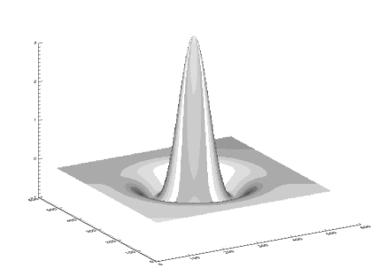
Figure 7: MHW in real space. The size of the grid over which the MHW is defined in this plot is $30^{\prime}\times 30^{\prime}$. Although the scale, $s$, of this MHW is 3 arcmin, then the total size of the MHW is $\approx 20$ arcmin.

In a few words, the effect of the MHW is to magnify, with respect to the background, the signals with scales around the scale of the MHW. The idea is to look at the number of wavelet coefficients above a certain level (threshold) at different scales in the map of CMB plus SZE residual (plus noise) and compare these coefficients with the ones obtained when only the CMB (plus noise) is considered. We show the result for the channel at 353 GHZ in Figure 8, where we have changed the scale just to see how the contribution of the SZE residual changes with the scale of the MHW. In our simulations, we have also included the expected Planck noise level in this channel. The instrumental noise is simulated as a white Gaussian noise with an RMS of $14.4\times 10^{-6}$ per resolution element in $\Delta T/T$ units. The result is compared with the mean value and $1\sigma$ error bars obtained from 100 Gaussian realizations of the CMB (plus instrumental noise). The mean value of these realizations is consistent with the expected number of wavelet coefficients (in absolute value) above the threshold for a map with $512^{2}$ MHW coefficients. This expected number is just $0.0465\%$ (for a threshold = $3.5\sigma$) of $512^{2}$ which is $\approx$ 120. This number is a constant independent of the scale of the MHW since the convolution of the CMB maps with the MHW does not change their Gaussian nature. Since the original map contains $512^{2}$ pixels, the convolved map will contain $512^{2}$ MHW coefficients and the expected number of MHW coefficients (in absolute value) above $3.5\sigma$ for a Gaussian map will remain constant at all scales, $\approx$ 120. The reason why we choose a threshold of $3.5\sigma$ is because we have to find a compromise between having enough statistics and the significance of the result. A lower threshold will produce a larger number of coefficients above the threshold but these number will be more dominated by the Gaussian part of the distribution. A higher threshold will select the tail of the Gaussian distribution which will show more clearly the non-Gaussian contribution due to the SZE residual. However, a high threshold will have a low expected number of coefficients above the threshold in a Gaussian case. We choose the threshold at $3.5\sigma$ because for this threshold, both the mean number of Gaussian coefficients and the significance are high enough (120 and $3.5\sigma$ respectively).

Figure 8: Number of MHW coefficients above $3.5\sigma$ level as a function of the scale of the MHW for two Planck channels, 353 GHz (left) and 143 GHz (right). The solid line is the number of coefficients (in absolute value) above the threshold for the Gaussian CMB map plus the SZE residual plus noise. For reference, we also show the case when the SZE is not removed at all (dotted line). The big black dots are the mean value of 100 Gaussian realizations of the CMB plus the corresponding noise at that channel and the error bars are $1\sigma$. The mean value is consistent with the expected number of points above $3.5\sigma$ for a map with $512^{2}$ wavelet coefficients (in absolute value). This plot clearly shows, how the residual adds a significant ($>4\sigma$) non-Gaussian signature at small scales in the 353 GHz channel. In the case of the 143 GHz channel, the SZE residual does not introduce a significant non-Gaussian signature. In the rest of the channels, the number of coefficients above $3.5\sigma$ are also consistent with the Gaussian case.

As it can be seen in figure 8, the CMB plus SZE residual shows a clear deviation from the Gaussian case which is larger when the scale is smaller. The deviation is maximum at scales of the MHW around 3 arcmin ($4.25\sigma$ at 2.8 arcmin). For the rest of the channels, the non-Gaussian signature of the CMB plus SZE residual is consistent (within the corresponding error bars) with the Gaussian case (see the 143 GHz case). This is due to two things. First, the amplitude of the SZE residual is smaller in the other channels. Second, and more important, the antenna is larger and the signal is diluted so the small scales cannot be magnified with the same efficiency as in the channel at 353 GHz. For comparison we show the result when our Gaussianity estimator is applied to the 143 GHz channel. In this case, no significant non-Gaussianity is observed at small scales. In the rest of the channels, the antenna is even larger so the dilution of the residual is bigger. The main conclusion is that the 353 GHz channel can contain a significant non-Gaussian signal at small scales coming for the SZE residual. It is worth pointing out, that MAP will not measure non-Gaussianity from SZE residuals mainly because of the lower resolution, $\sim 12$ arcmin at $90$ GHz (i.e. the situation will be similar to what we observe in the channels below 143 GHz).
It is also worth pointing out that such non-Gaussianity studies could be used to determine which component separation methods are most useful for Planck. In future works focusing on non-Gaussianity studies, one could imagine using the 353 GHz channel to remove the non-Gaussianity due to SZE residuals from the other channels. Another interesting possibility is to use this non-Gaussianity to remove even more of the SZE residual.

In Figure 9 we show the histogram of the two wavelet coefficient maps (CMB plus noise and CMB plus noise plus SZE residual) for the case when the maps are filtered with a MHW with a scale of 3 arcmin. This plot shows again the non-Gaussian nature of the CMB plus SZE residual map at small scales.

Figure 9: Histograms of the 3 arcmin MHW coefficient maps. The dotted line is the case when only the CMB plus noise is considered (no residual). The solid line shows the excess when the the SZE residual is added to the CMB plus noise map (353 GHz channel).

We have also applied our non-Gaussianity estimator to see if we can detect some non-Gaussianity coming from the contribution of the kinematic SZE. We did not find any non-Gaussian signatures due to this component.

6 Conclusions

In this paper we have studied the systematic errors introduced in the Planck cluster catalogue and in the CMB map due to the imperfect SZE subtraction caused by the non-relativistic assumption and to the intrinsic error in the component separation process. We have used the non-parametric method proposed in [Diego et al. 2002] to perform the component separation method. This method is very robust in the sense that it makes a minimum number of assumptions. The drawback is that it is not the most precise in the determination of the SZE component. However, this allow us to put an upper limit on the systematic errors introduced by the imperfect SZE subtraction since any more sophisticated method in principle should produce smaller SZE residuals.

We have seen that the effect of the non-relativistic assumption in the frequency dependence of the SZE made in the component separation process is small when compared to the case where the real frequency dependence is assumed (between 4% and 8% relative difference for $T=10$ keV clusters), however, the relativistic corrections should be considered in the simulations of the SZE in order to compute correctly the selection function and completeness level of the cluster catalogue.

Concerning the kinematic component of the SZE, relativistic corrections should be taken into account in order to recover this component. Otherwise errors as large as $50-100\%$ could be introduced in this component in the most relevant channel for its detection (217 GHz).

In the CMB, the SZE residual in the 353 GHz leaves a non-Gaussian signature at small scales which could be detected by some Gaussianity estimators like the MHW. This channel could thus be used to extract non-Gaussianity signatures from imperfect SZE subtraction from the other channels. Our MHW Gaussianity estimator does not show significant deviations from Gaussianity due to imperfect SZE recovery in the other channels relevant to the CMB.

The SZE residual does not change significantly the power spectrum of the CMB in the 353 GHz channel. It is therefore safe to include the 353 GHz channel for the computation of the CMB power spectrum. This channel, together with the 217 GHz channel, are the most important ones which will contribute to the CMB map at the smallest scales ($\approx 5$ arcmin).

References

- [Aghanim & Forni 1999] Aghanim N. & Forni O., 1999, A&A. 347, 409.
- [Aghanim, Gorski & Puget 2001] Aghanim N., Gorski, K. M., Puget, J.-L., 2001, A&A. 374, 1.
- [Bertin & Arnouts 1996] Bertin, E. & Arnouts, S. 1996, A&AS, 117, 393.
- [Birkinshaw 1999] Birkinshaw M., 1999, Phys. Rep. 310, 97.
- [Bouchet & Gispert 1999] Bouchet F. & Gispert R., 1999, New Astronomy, 4-6, 443.
- [Carlstrom et al. 2001] Carlstrom J. E. et al., 2001, Constructing the Universe with Clusters of Galaxies, IAP conference, July 2000, eds. F. Durret and G. Gerbal.
- [Challinor & Lasenby 1998] Challinor A., Lasenby A., 1998, Astrophys. J. 499, 1.
- [Cooray 2001] Cooray A., 2001, Phys. Rev. D, 64, 063514.
- [Diego et al. 2001] Diego J. M., Martínez-González E., Sanz J.L., Cayón L., Silk J. 2001, MNRAS, 325, 1533.
- [Diego et al. 2002] Diego J.M., Vielva P., Martínez-González E., Silk J., Sanz J.L. , 2001. MNRAS in press. preprint (astro-ph/0110587)
- [Dolgov et al. 2001] Dolgov A. D., Hansen S. H., Pastor S., Semikoz D.V., 2001, Astrophys. J. 554, 74.
- [Enqvist et al. 2000] Enqvist K., Kurki-Suonio H., Valiviita J., 2000, Phys. Rev. D, 62, 103003.
- [Hansen, Pastor & Semikoz 2002] Hansen S. H., Pastor S., Semikoz D. V., 2002, Astrophys. J. 573, L69.
- [Herranz et al. 2001] Herranz D., Sanz J.L., Hobson M.P., Barreiro R.B., Diego J.M., Martinez-Gonzalez E., Lasenby A.N., 2001, MNRAS submitted. preprint (astro-ph/0203486).
- [Hobson et al. 1998] Hobson M.P., Jones A.W., Lasenby A.N., Bouchet F.R., 1998, MNRAS, 300, 1.
- [Itoh, Kohyama & Nozawa 1998] Itoh N., Kohyama Y., Nozawa, S., 1998, Astrophys. J. 502, 7.
- [Itoh et al. 2001] Itoh N., Kawana Y., Nozawa S., Kohyama Y., 2001, MNRAS 327, 567.
- [Peebles 1980] Peebles P.J.E., 1980. ‘The large scale structure of the Universe. Princeton University Press.
- [Pointecouteau, Giard & Barret 1998] Pointecouteau E., Giard M., Barret D., 1998, Astron. Astrophys. 336, 44.
- [Press & Schechter 1974] Press W., Schechter P, 1974, Astrophys. J., 187, 425
- [Rephaeli 1995] Rephaeli Y., 1995, Astrophys. J. 445, 33.
- [Rephaeli 2001] Rephaeli Y., 2001, preprint (astro-ph/0110510).
- [Sanz et al. 2001] Sanz J. L., Herranz D., Martinez-Gonzalez E., 2001, ApJ, 552, 484.
- [Stebbins 1997] Stebbins A., 1997, preprint (astro-ph/9709065).
- [Sunyaev & Zeldovich 1972] Sunyaev R. A., Zel’dovich Ya. B., 1972, Comments Astrophys. Space Phys. 4 173.
- [Tegmark & Efstathiou, 1996] Tegmark M., & Efstathiou G., 1996 MNRAS, 281,1297.
- [Tegmark & de Oliveira-Costa, 1998] Tegmark M., & de Oliveira-Costa A., 1998, ApJ, 500, L83.
- [Wright 1979] Wright E. L., 1979, ApJ, 232, 348.
- [Yoshida et al. 2001] Yoshida N., Sheth R.K., & Diaferio A., 2001, MNRAS, 328, 669.