A Far-Ultraviolet Survey of 47 Tucanae. I. Imaging

Abstract

We present results from the imaging portion of a far-ultraviolet (FUV) survey of the core of 47 Tucanae. We have detected 767 FUV sources, 527 of which have optical counterparts in archival HST/WFPC2 images of the same field.

Most of our FUV sources are main-sequence (MS) turn-off stars near the detection limit of our survey. However, the FUV/optical color-magnitude diagram (CMD) also reveals 19 blue stragglers (BSs), 17 white dwarfs (WDs) and 16 cataclysmic variable (CV) candidates. The BSs lie on the extended cluster MS, and four of them are variable in the FUV data. The WDs occupy the top of the cluster cooling sequence, down to an effective temperature of $T_{eff}\simeq 20,000$ K. Our FUV source catalog probably contains many additional, cooler WDs without optical counterparts. Finally, the CV candidates are objects between the WD cooling track and the extended cluster MS.

Four of the CV candidates are previously known or suspected cataclysmics. All of these are bright and variable in the FUV. Another CV candidate is associated with the semi-detached binary system V36 that was recently found by Albrow et al. (2001). V36 has an orbital period of 0.4 or 0.8 days, blue optical colors and is located within 1 arcsec of a Chandra x-ray source. A few of the remaining CV candidates may represent chance superpositions or SMC interlopers, but at least half are expected to be real cluster members with peculiar colors. However, only a few of these CV candidates are possible counterparts to Chandra x-ray sources. Thus it is not yet clear which, if any, of them are true CVs, rather than non-interacting MS/WD binaries or Helium WDs.

1 Introduction

Globular clusters (GCs) are fantastic stellar crash test laboratories. Violent encounters between binaries and single stars in dense cluster cores give rise to exotic stellar populations, such as blue stragglers (BSs), cataclysmic variables (CVs), low-mass x-ray binaries and milli-second pulsars. All of these objects have considerably bluer spectral energy distributions than the non-degenerate stars that make up the bulk of the GC mass. Observations at short wavelengths are thus ideally suited to the detection and characterisation of these relatively rare stellar species. This is nicely illustrated by the recent Chandra survey of 47 Tuc (Grindlay et al. 2001a), which finally showed that the theoretically predicted, extensive population of interacting close binaries really does exist there. Nevertheless, important puzzles still remain. For example, even though Grindlay et al. (2001a) estimated that there are 30 CVs with $L_{x}\raisebox{-2.58334pt}{$\,\stackrel{{\scriptstyle\raisebox{-0.60275pt}{$\textstyle>$}}}{{\sim}}\,$}10^{30}$ ergs s^-1 in 47 Tuc – far more than found in any previous study – this is at best 1/3 of the number predicted by tidal capture theory (Di Stefano & Rappaport 1994).

Given the striking differences between optical and Chandra x-ray images of 47 Tuc, it seems clear that observations at intermediate wavelengths – i.e. the far-ultraviolet (FUV) – would be invaluable in identifying and characterising both the Chandra sources and other exotic objects in the cluster. For example, it is well known that CVs and young white dwarfs (WDs) radiate much of their luminosity in the FUV waveband. We have therefore embarked on a program to study the cores of nearby GCs at FUV wavelengths, using both imaging and slitless spectroscopy. The extraordinary spatial resolution and FUV sensitivity of the Space Telescope Imaging Spectrograph (STIS) aboard the Hubble Space Telescope (HST) make this the instrument of choice for our study. Here, we present first results from a campaign on 47 Tuc, which clearly demonstrate the value of FUV observations to the study of GCs.

2 Observations and Data Reduction

2.1 FUV Photometry

Thirty orbits of STIS/HST observations of 47 Tuc have been obtained, comprised of six epochs of five orbits each (HST program GO-8219). In each epoch, we carried out FUV imaging and slitless spectroscopy. Consecutive observing epochs were as closely spaced as a few days and as widely separated as a year. Typical exposure times in the FUV were 600 s. Our program is therefore sensitive to variability on time-scales ranging from minutes to months. In this first paper arising from our survey, we will focus on the results obtained from the FUV imaging aspect of the program; the analysis of the slitless spectroscopy is in progress and will be presented elsewhere.

All of our FUV observations (both imaging and spectroscopic) used the FUV-MAMA detectors and were taken through the F25QTZ filter. The purpose of this filter is to block geocoronal Ly$\alpha$, OI 1304 Å and OI] 1356 Å emission which would otherwise produce a high background across the detector in our slitless spectroscopy. The effective bandpass with this instrumental set-up is 1450 Å – 1800 Å. The 1024$\times$1024 pixel FUV-MAMA detector covers approximately 25″$\times$25″, at a spatial resolution of about 0.043″ (FWHM). Our field of view (FoV) was chosen to overlap with archival HST observations of 47 Tuc and included the cluster center.

Source detection and photometry was carried out on a deep FUV image that was constructed by registering and co-adding all of the individual FUV imaging exposures. We note that – like x-ray detectors, but unlike optical CCDs – the FUV/MAMAs are photon counting devices with no read noise and very little dark current (approximately $7\times 10^{-6}$ c s^-1 pix^-1). As a result, sky and faint source pixels tend to show either exactly zero or one count in a typical FUV exposure. This implies that median filtering is a sub-optimal way of combining multiple FUV exposures. Instead, FUV images should be combined by direct summing or averaging.

We obtained two FUV imaging exposures at the beginning and end of each observing epoch, for a total of 24 FUV images. The registration and co-addition of these images was performed with routines available in the iraf/images package. In doing so, we took care to mask known image defects (e.g. hot pixels) by inspecting the data-quality file associated with each individual exposure. The final, deep FUV image corresponds to a total exposure time of approximately 14,600 s.

Source detection and photometry on the co-added FUV image was carried out with the SExtractor software (Bertin & Arnout 1996). This was preferred to other packages because our FUV images share characteristics with both standard CCD images (e.g. compact PSF) and x-ray images (e.g. low background, complex PSF shape). The software of choice has to work well with both types of characteristics, and the SExtractor fits this bill: it was designed primarily for use with CCD images, but is also known to work well on x-ray images (Valtchanov, Pierre & Gastaud 2001).

The SExtractor uses a matched filtering method for source detection. When dealing with CCD images, it is usually sufficient to use a simple analytic filter (e.g. a Gaussian) whose width is chosen to match that of the detector point spread function (PSF). However, the FUV/MAMA PSF is quite complex and asymmetric. We therefore designed our own matched filter from an empirical PSF that was constructed using the daophot package within iraf.

The detection threshold within SExtractor was set to 5$\sigma$ above the local background, with the minimum source area set to 5 pixels. However, it is important to note that these numbers refer to the filtered image. A more transparent way to characterise our detection threshold is to consider the completeness of our source detection procedure as a function of magnitude. As described in Section 2, artificial star tests suggest that our FUV survey is almost complete to $m_{FUV}\simeq 24$. Here, $m_{FUV}$ is the FUV magnitude of a source in the STMAG system, defined by

$$m_{FUV}=-2.5\log{F_{\lambda}}-21.1,$$ (1)

where $F_{\lambda}$ is the flux of a hypothetical flat-spectrum source. Thus $m_{FUV}\simeq 24$ corresponds to $F_{\lambda}\simeq 9\times 10^{-19}$ ergs cm^-2 s¹ Å^-1. In terms of recorded counts, we have

$$F_{\lambda}=\frac{{\rm Counts}\times{\rm PHOTFLAM}}{{\rm Exposure~{}Time}},$$ (2)

where PHOTFLAM ($=1.04\times 10^{-16}$ ergs cm^-2 Å^-1 counts^-1 for our set-up) is the inverse sensitivity of the detector/filter combination. Given the effective exposure time of the co-added FUV frame, our $m_{FUV}\simeq 24$ completeness threshold corresponds to approximately 125 source counts; about 80 of these fall within our photometric aperture (see below). Thus our detection threshold corresponds to $S/N\simeq 9$ at the completeness limit. As a last step, we rejected sources that were too close to the image edges, resulting in a final catalog of 767 FUV sources.

Since the FUV image is not particularly crowded, we were able to use simple aperture photometry to measure the magnitudes of the detected FUV sources. All FUV magnitudes quoted below are on the STMAG system and were calculated using an aperture with a radius of 5 pixels. The aperture correction to infinite radius was estimated using both empirical and theoretical PSFs. The theoretical PSF was calculated with the TinyTim software.

We also carried out a search for variability among our FUV sources. This was done by registering individual FUV frames to the co-added frame and performing aperture photometry at the positions of the previously detected FUV sources on these frames. Likely variables were identified by calculating the standard deviation, $\sigma$, of each light curve and searching for outliers in a plot of $\sigma$ vs $m_{FUV}$. Candidate variables were then inspected by eye on the images and removed from the list if their variability appeared to be spurious (e.g. due to image defects or a location near the image edges). This procedure finally allowed us to identify 8 FUV sources that appear to be genuinely variable. These will be discussed in more detail in Section 3.

2.2 Optical Photometry

In order to find optical counterparts for our FUV sources, we used the HST archive to construct a deep U-band image of the STIS FoV. More specifically, we extracted from the HST archive all WFPC2/PC/F336W ($\simeq$ U) exposures that contained at least part of our FoV. We registered and combined these images, and carried out source detection and PSF-fitting photometry on the co-added frame using daophot (Stetson 1987). Magnitudes were again placed on the STMAG system, but it is important to note that stars brighter than $m_{336}\simeq 16$ were generally saturated in the co-added frame. At the other extreme, the optical photometry is not sensitive to objects fainter than $m_{336}\simeq 22-23$.

2.3 Matching FUV and Optical Catalogs

We also extracted and combined all WFPC2/PC/F218W images covering our FoV from the HST archive. Even for the bluest objects (hot WDs), the co-added F218W image does not go as deep as the co-added F336W image. However, the F218W bandpass lies between the STIS/FUV/F25QTZ and WFPC2/F336W bandpasses, making the F218W frame a useful intermediary in the process of matching up FUV and F336W sources. Ferraro et al.’s (2001) list of BSs, hot WDs and UV-excess stars in the core of 47 Tuc provided a particularly convenient starting point in this context. These authors provide F218W positions for all objects on their list, many of which turn out to be detectable in both FUV and F336W. Starting with this initial list of matches, we iteratively improved the transformation between F336W and FUV positions by finding additional matches and rederiving transformation coefficients. With our final transformation, there are 4894 U-band sources within our effective FUV FoV.

In our search for optical counterparts, we adopted a maximum difference of 1.5 STIS/FUV-MAMA pixels ($\simeq 0.038\arcsec\simeq 0.8$ WFPC2/PC pixels) between the centers of FUV sources and their F336W counterparts. Even with this conservative criterion, we managed to find counterparts to 527 FUV sources. We chose such a restrictive matching radius in order to keep the likely number of false matches at an acceptable level. This is an important consideration, since with 767 FUV and 4894 optical sources sharing approximately 1 million pixels, we certainly expect some false matches to occur. The expected number of false matches depends on the numbers of objects in the two source lists, the matching tolerance and the actual number of objects matched. Based on these parameters, we estimate that our list of optical counterparts contains approximately 8 false matches overall, but only 3 among FUV sources brighter than $m_{FUV}=22$. This distinction is important because most of the interesting objects in our CMD are brighter than this limit.

3 Results and Discussion

3.1 Comparison of FUV, Optical and X-ray Imaging

In Figure 1, we show a comparison of the F336W and FUV images of the same 25″$\times$25″ field near the core of 47 Tuc. The optical image is vastly more crowded, because the majority of main-sequence stars, red giants and horizontal branch stars are too cool to show up in the FUV exposure. We have overlayed onto the FUV image the predicted positions of known, blue sources from Geffert, Auriére & Koch-Miramond (1997) and also the predicted positions of the Chandra x-ray sources from Grindlay et al. (2001a). In both cases, the positions were determined by first placing the sources on the F336W frame, using the invmetric task within iraf/stsdas, then improving these positions by using three sources that are common to both lists and are also detected in both our F336W and FUV frames. These three sources are AKO9 [W36], V1 [W42, X9] and V2 [W30, X19] (the identifications in square brackets refer to alternative designations in the literature; ’W’ numbers, in particular, refer to Table 1 of Grindlay et al. 2001a; ‘X’ numbers refer to Table 2 of Verbunt & Hasinger 1998). We finally transformed the positions to the STIS/FUV frame, using our previously derived transformation.

Figure 1 shows that almost all of the blue sources listed by Geffert et al. (1997) have certain or likely FUV counterparts. This was to be expected, but is nevertheless important: it provides an external check on our astrometry and supports our contention that FUV imaging is an excellent way of finding interesting GC sources. We find fewer obvious FUV counterparts to the Grindlay et al. (2001a) x-ray sources within our FoV. This is not so surprising, given that approximately 70% of their sources are expected to be very faint FUV sources (millisecond pulsars and x-ray active main sequence binaries). A more interesting question is whether we detect those Chandra sources that are definitely expected to be FUV bright. There are only four such sources in our FoV, all of which were classified by Grindlay et al. as CVs. Three of these are thought to be associated with previously known or suspected CVs, namely our reference stars AKO 9, V1 and V2; all three are also clearly detected in our FUV images. The fourth source – denoted W15 by Grindlay et al. (2001a) – is a CV candidate that was not known prior to the Chandra survey of 47 Tuc. It, too, has a likely counterpart in our FUV images (see Figure 1 and Section 3.3.5).

3.2 The FUV luminosity function

In Figure 2, we show the FUV luminosity function (LF) for the 767 stars we detected in our FUV image. The main feature of the LF is the sharp rise towards $m_{FUV}\simeq 24$. As we will show below, this feature is due to main-sequence turn-off (MSTO) stars which become detectable near this magnitude. A second interesting aspect of the LF is that the brightest source in the sample earns that distinction by a considerable margin (approximately 1.75 mags). This source is AKO 9, which we will return to in Section 3.3.5 below.

In order to assess the completeness of our sample, we used the addstar routine within daophot to carry out artificial star tests. The results are shown in the top panel of Figure 2 and suggest that our survey is close to complete to roughly $m_{FUV}\simeq 24$. However, it is worth noting that (i) both addstar and SExtractor used the same PSF, and (ii) the addstar routine does not account for the quantization of counts at low count levels. As a result, our completeness estimates could be slightly optimistic.

3.3 The FUV/Optical Color-Magnitude Diagram

In Figure 3, we present the FUV-optical color-magnitude diagram (CMD) of 47 Tuc. Several distinct stellar populations are present in CMD, among them WDs, BSs, MSTO stars and, last but not least, CVs. We have also calculated and plotted a set of theoretical tracks whose purpose is to aid in the interpretation of the CMD. We will first describe the calculation of these tracks and then discuss the implications of our CMD for our understanding of the stellar populations within it.

3.3.1 Synthetic Photometry

The starting point for our synthetic photometry was the recent work by VandenBerg (2000), who modelled the optical CMD of 47 Tuc. Don VandenBerg kindly provided us with the corresponding set of isochrones and zero-age horizontal branch (ZAHB) models, from which we extracted the stellar parameters of main sequence stars, sub-giants, red giants and horizontal branch stars in 47 Tuc. We then used synphot within iraf/stsdas to calculate the FUV and optical magnitudes of stars on these sequences. This was achieved by interpolating on the Kurucz grid of model stellar atmospheres and folding the resulting synthetic spectra through the response of the appropriate filter+detector combinations. The cluster parameters we adopted in our calculations are those of VandenBerg (2000), i.e. $E(B-V)=0.032$, $d=4510$ pc, ${\rm[Fe/H]}=-0.83$ and ${\rm[\alpha/Fe]}=0.3$. VandenBerg’s study puts 47 Tuc’s age at approximately 11.5 Gyr, so we calculated isochrones for 10, 12 and 14 Gyr.

We also calculated an approximate BS sequence for our CMD. For this, we assumed BSs to lie near the zero-age main sequence (ZAMS) of the cluster, and used the fitting formulae of Tout et al. (1996) to estimate the appropriate stellar parameters. The corresponding FUV and optical colors were again estimated from the Kurucz model grid within synphot. The same technique was used to estimate the location of the ZAMS of the Small Magellanic Cloud (SMC), which is relevant because 47 Tuc is located in front of the SMC. For the SMC, we adopted a metallicity of ${\rm[Fe/H]}=-0.68$, a distance of 58.6 kpc and the same reddening as for 47 Tuc (Böhm-Vitense 1997). We also calculated a theoretical WD cooling sequence for our CMD. In doing so, we adopted a mean cluster WD mass of 0.53 M_⊙ (Renzini & Fusi-Pecci 1988) and used DA WD model atmospheres to calculate the predicted colors. For models with $T_{eff}\leq 15,000$ K, we used a small grid of model atmospheres calculated with tlusty/synspec (Hubeny, Lanz & Jeffery 1994) and kindly provided to us by Ivan Hubeny. For models with higher $T_{eff}$, we used the Vennes et al. (1993) grid of DA WD models, which was kindly provided to us by Stephane Vennes.

3.3.2 Main-sequence stars, sub-giants, red-giants and horizontal branch stars

Returning to Figure 3, we first note the prominent clump of stars in the upper right quadrant. This clump contains most of the stars in the CMD and happily coincides almost exactly with the expected location of the MSTO.

We next focus on the smaller clump of stars near the predicted location of the ZAHB (i.e. above and to the blue of the MSTO). This second clump (at $m_{F336W}\raisebox{-2.58334pt}{$\,\stackrel{{\scriptstyle\raisebox{-0.60275pt}{$\textstyle<$}}}{{\sim}}\,$}16$) contains mostly saturated horizontal branch stars (c.f. Section 2.2); i.e. its apparent location below the ZAHB track is an artifact of saturation.

Finally, there is also a trail of stars between these two clumps, which cannot be explained as an artifact due to saturation. We have therefore used additional archival data to investigate the nature of the sources on this trail and find that they are red giants. For comparison, the synthetic red giant branch is approximately 4-5 magnitudes redward of this trail.

In order to understand this apparent discrepancy, it is important to realize that our CMD does not imply that these stars are FUV bright, only that they are not as FUV faint as stellar atmosphere models predict. This is not particularly surprising. After all, the Kurucz model atmospheres include only the photospheric stellar flux. However, the FUV waveband is well down the Wien tail of a red giant’s photospheric spectrum, so that chromospheric emission can totally dominate the FUV output of these systems. Figure 1 of Robinson, Carpenter & Brown (1998) nicely illustrates this effect for two isolated K Giants. We finally note that the chromospherically-dominated FUV spectra of red giants are rich in emission lines; these might be detectable in our slitless spectroscopy.

3.3.3 Blue Stragglers

The BS sequence can be seen as a trail of stars starting at the MSTO and going upwards and to the left. The slight discrepancy between the observed BS sequence and the synthetic one is not surprising, since the latter assumes that the BSs lie on the ZAMS. In reality, BSs may be expected to be somewhat evolved, explaining their location above and to the red of the ZAMS. In total, there are 19 BSs in our CMD, extending all the way from the MSTO (at approximately 0.9 M_⊙) to perhaps 1.5 M_⊙ (judging from the ZAMS models). Four of these (circled in Figure 3) appear to be variable in our FUV photometry. This is plausible, given that variability is a known phenomenon among BSs (e.g. Gilliland et al. 1995).

3.3.4 White Dwarfs

The WD cooling sequence is clearly visible in the bottom left quadrant of the CMD. The faintest WDs on this sequence have $T_{eff}\simeq 20,000$ K, but it is worth noting that this detection limit is imposed by the depth of the optical data. Indeed, our FUV detection limit of $m_{FUV}\simeq 24$ corresponds to a WD with $T_{eff}\simeq 11,500$ K.

It is interesting to ask whether the numbers of WDs we detect are in line with expectations. A simple estimate of the expected number can be made following Richer et al. (1997). The number of stars in two post-main-sequence phases is, in general, proportional to the duration of these phases. We will use horizontal branch (HB) stars as a reference point, and take $N_{HB}$ as the number of HB stars in our FoV and $\tau_{HB}\simeq 10^{8}$ yrs as their lifetime (e.g. Dorman 1992). We then expect to find approximately

$$N_{WD}(T_{eff}>T_{lim})\simeq N_{HB}\times\left[\frac{\tau_{WD}(T_{lim})}{\tau_{HB}}\right],$$ (3)

WDs hotter than $T_{lim}$ in the FoV, where $\tau_{WD}(T_{lim})$ is the time it takes a WD to cool to $T_{lim}$. Inspection of published optical observations shows that $N_{HB}\simeq 50$ (Guhathakurta et al. 1992). We note that the estimate in Equation 3 ignores the effect of mass segregation. This is a reasonable first approximation in our case, since the cooling time-scales among our WD population are short and comparable to the core relaxation time of $\sim 10^{8}$ yrs [Harris 1996]).

For a first check, we will assume that the 17 WDs in our CMD represent the complete WD population in our FoV down to $T_{eff}\simeq 20,000$ K. The true number is likely to be higher, since our optical data is likely to be seriously incomplete at the faint end of the WD sequence. If we nevertheless adopt this assumption and use the models of Althaus & Benvenuto (1998) to estimate the corresponding cooling time, we find $\tau_{WD}\simeq 5\times 10^{7}$ yrs and hence $N_{WD}(T_{eff}>20,000{\rm~{}K})\simeq 25$. As expected, this is slightly larger than the observed number, but in the right ballpark. A second estimate can be made by assuming that all FUV sources with $m_{FUV}<22$ (corresponding to $T_{eff}\simeq 14,500$ K) are WDs, unless their location in the CMD contradicts this. This allows us to include sources without optical counterparts, on the assumption that all such sources are optically faint WDs. There are a total of 121 FUV sources satisfying $m_{FUV}<22$ in our catalog, 34 of which are clearly not single WDs (based on their location in the CMD). We therefore estimate that the number of WDs with $T_{eff}>14,500{\rm~{}K}$ is 87. The true number is probably somewhat lower, since some of the FUV sources without optical counterparts may, for example, be faint CVs (see below). The cooling time for this temperature is roughly $1.8\times 10^{8}$ yrs and hence the predicted number of WDs is $N_{WD}(T_{eff}>14,500{\rm~{}K})\simeq 90$. Observed and predicted numbers appear to be in reasonable agreement.

3.3.5 Cataclysmic Variables

We finally turn to the CV candidates that are revealed by our CMD. Given that CVs are binary systems containing an accreting WD and (usually) a MS star, we expect them to be located between the WD cooling sequence on one side and the MS (and its BS extension) on the other. We will refer to this area of the CMD as the “CV zone”. There are 16 objects in the CV zone, not including the star just off the lower left of the MSTO. How many of these sources are likely to be real CVs?

We first note that four objects in the CV zone – AKO 9, V1, V2 and W15 – are already confirmed CVs. All four of these sources are FUV bright and variable, and all four are Chandra x-ray sources that were also classified as CVs by Grindlay et al. (2001a). In the case of AKO 9 and V2, our slitless spectroscopy has already provided spectroscopic confirmation as well, via the detection of FUV emission lines (Knigge et al., in preparation; see Knigge et al. 2002 for a preliminary report). The identification of AKO 9 as a CV is especially important, since the nature of this 1.1-day binary had been unclear since its discovery by Auriére, Koch-Miramond & Ortolani (1989). A more detailed description of our FUV data on this source is in preparation.

Another one of our CV candidates also deserves special mention. This is the source labelled as V36 in both Figures 1 and 3. This identification follows the notation of Albrow et al. (2001), who show that V36 is likely to be a semi-detached binary system with an orbital period of 0.4 or 0.8 days. V36 was previously classified as a BS by Paresce et al. (1991) and has also been noted as an unusually blue source by De Marchi, Paresce & Ferraro (1993), Geffert et al. (1997) and Ferraro et al. (2001). Based on the FUV imaging and astrometry shown in Figure 1, we now find that V36 is also a strong FUV emitter and located within 1 arcsec of a Chandra x-ray source. We therefore suggest that V36 is a strong CV candidate (see, however, the note added at the end of this paper).

Turning to the remaining 11 sources in the CV zone, we first consider the possibility that some of them are due to chance superpositions of physically unrelated WDs and MS stars. All of the sources are relatively FUV bright ($m_{FUV}\raisebox{-2.58334pt}{$\,\stackrel{{\scriptstyle\raisebox{-0.60275pt}{$\textstyle<$}}}{{\sim}}\,$}22$) and therefore located in a region of the CMD where we should expect only about 3 false matches (c.f. Section 2.3). The resulting spurious sources would most likely be located near the peak of the optical luminosity function, i.e. around $m_{336}\simeq 18$ (e.g. Howell et al. 2001). Thus any false matches amongst the objects in the CV zone are most likely to come from the 7 sources with $m_{336}<20$ and $m_{FUV}-m_{336}>0$. However, only three of these – the three CV candidates closest to V36 in the CMD – show an offset in excess of 1 pixel between FUV and optical positions.

A second point to consider is whether some of the objects in the CV zone may be background stars in the SMC halo behind 47 Tuc. The expected location of the SMC ZAMS is indicated on the CMD. However, it is important to note that the bulk of SMC stars in this region follows an isochrone whose MSTO lies at about $m_{336}\sim 22.5$ (c.f. Zoccali et al. 2001). The likely degree of SMC contamination in our data can be quantified by comparison with the HST/WFPC2 observations of Zoccali et al. (2001). Their FoV covers approximately 17,000 arcsec² centered 6.5′ west of the cluster center. Within this field, there are perhaps 10 possible SMC interlopers brighter than $m_{336}\sim 22.5$ (see their Figure 1, but note that their quoted magnitudes are instrumental). Scaling this number to the area covered by our roughly 630 arcsec² FoV, we may expect to find about 0.4 SMC interlopers in our CMD. Even allowing for small number statistics, it is unlikely that there are more than one or two SMC stars in the CV zone.

The third question we must ask is whether some of the objects in the CV zone are affected by blending, image defects, edge effects, etc in the FUV image. We have therefore inspected by eye the positions of all 16 objects in the co-added FUV image (c.f. Figure 1). Based on this, the two sources closest to the BS sequence within the CV zone deserve further comment. One of them lies quite close to an image edge, but our aperture photometry for it should not be compromised significantly. In any case, we would expect edge effects to reduce the apparent brightness of this source, i.e. any correction would probably make this object appear even bluer and thus move it further into the CV zone. The other object lies within a few pixels of a fainter FUV source. This may have led to a mild overestimate of its FUV brightness, but the shift required to bring it close to the MSTO (about 2 mags) appears to be much larger than any implied correction.

Fourth, we have to look more carefully at our definition of the “CV zone”. More specifically, we must ask if the colors of the objects in this zone are actually consistent with those of CVs. We have addressed this question by plotting the locations of several proto-typical field CVs in our CMD, after placing these systems at the distance and reddening of 47 Tuc. The FUV magnitudes of the field CVs were calculated by running their IUE spectra through synphot; their F336W colors were estimated from U-band magnitudes in the literature (primarily Bruch & Engel 1994). Some field CVs appear twice in Figure 3, representing the same object in different states (e.g. dwarf novae in quiescence and outburst). We stress that this comparison between cluster CV candidates and field CVs is fraught with uncertainties, since the stellar environments and parameters of the two types of CVs are quite different. Nevertheless, it is clear from Figure 3 that most of the cluster sources in the CV zone of the CMD lie reasonably close to the positions of field CVs. The comparison also shows that the spectrum of some field CVs, like AM Her, can at times be dominated by their WDs, in both FUV and U/F336W bandpasses. This means that a few of the FUV sources on the WD cooling track may yet turn out to be CVs.

Fifth and finally, we must look at other types of stars that may be found in the CV zone, such as non-interacting MS/WD binaries. Indeed, given that there may be $\simeq 90$ young WDs down to $m_{FUV}\simeq 22$ (Section 3.3.4) and that the binary frequency in the core of 47 Tuc is about 15% (Albrow et al. 2001), all of the unconfirmed CV candidates could be non-interacting MS/WD binaries. Another stellar type that may occupy the CV zone are Helium WDs, which have, for example, been found in NGC 6397 (Cool et al. 1998). Both MS/WD binaries and He WDs would be consistent with the apparent lack of FUV variability amongst our unconfirmed CV candidates.

Based on the discussion above, we conclude that (i) a conservative estimate for the number of “real” sources in the CV zone – as opposed to SMC interlopers, image defects and products of chance coincidences – is $N_{real}\simeq 10$; (ii) that the “CV zone” is a reasonable way to identify CV candidates; and (iii) that additional information will be needed to distinguish CVs from non-interacting MS/WD binaries and He WDs in the CV zone. With these conclusions in mind, we will consider both a best-case and a worst-case scenario. In the best-case scenario, the number of CVs in our CMD is $N_{CV}\simeq N_{real}\simeq 10$; in the worst-case scenario, none of the currently unconfirmed CVs will turn out to be real cataclysmics and $N_{CV}\simeq 5$. How do these numbers compare with theoretical expectations?

The simulations of Di Stefano & Rappaport (1994) predict that 47 Tuc should contain approximately 190 CVs that were formed by two-body tidal capture events (Fabian, Pringle & Rees 1975). Approximately half of these are expected to be located within one core radius of the cluster. Other CV formation channels exist (Davies 1997), but are probably less important than tidal capture in the cluster core. Given that our effective FoV samples approximately 35% of the 47 Tuc’s core ($r_{core}=23$″; Howell et al. 2001), our STIS image should contain roughly 30 CVs. However, many of these are predicted to be extremely faint, post-minimum period systems (“period-bouncers”), which we cannot hope to detect in our F336W data. This is confirmed by Figure 3, which shows that our F336W detection limit would not allow us to detect the most likely “period-bouncer” among field CVs – WZ Sge – in its normal, quiescent state. If we only count those CVs with predicted x-ray luminosities $L_{x}>10^{31}$ erg s^-1 in the model of Di Stefano & Rappaport (1994) – a rough dividing line between pre- and post-bounce CVs (c.f. their Figures 3 and 4) – the predicted number drops by roughly another factor of two. Thus the tidal capture models of Di Stefano & Rappaport (1994) predict that our CMD should contain approximately 15 CVs.

We conclude that if our optimistic estimate of $N_{CV}\simeq 10$ is correct, the observed-to-predicted ratio is about 2/3. This is not significantly different from unity, given the small number statistics involved. Thus the observed number of cluster CVs may, for the first time, be consistent with predictions based on tidal capture theory. But even in our worst-case scenario of $N_{CV}\simeq 5$, the observed-to-predicted ratio is still about 1/3. The same ratio was found by Grindlay et al. (2001a), based on their Chandra observations of the whole cluster.

We close this section by noting that only a few of our 11 unconfirmed CV candidates are located close to known x-ray sources (c.f. Figure 1). Assuming that this is not simply due to remaining uncertainties in the astrometry, there are two possible explanations for this. First, perhaps the worst-case scenario is close to the truth, and few or none of our new CV candidates are actually CVs. Second, our FUV survey is turning up new, x-ray faint CVs. Given the x-ray properties of field CVs (e.g. van Teeseling, Beuermann & Verbunt 1996) and the detection limit of the Chandra survey of 47 Tuc ($L_{x}\sim 10^{30}$ erg s^-1), this would be somewhat surprising. We may soon be able to decide between these possibilities on the basis of our time-resolved, slitless FUV spectroscopy.

4 Conclusions

We have presented first results from the imaging part of a FUV survey of 47 Tuc. The great benefit of moving to the FUV is that most ordinary cluster members are too cool to show up in this bandpass. This dramatically reduces crowding and makes it easy to find hot and/or exotic objects such as CVs, BSs and young WDs. The same lack of crowding even allows us to carry out slitless, multi-object FUV spectroscopy of the dense cluster core.

In this first analysis of our FUV observations of 47 Tuc, we have focused on the imaging aspect of our survey. By matching our FUV source catalog to a list of sources in a deep WFPC2/F336W ($\simeq$ U) image of the same field, we have been able to find 17 WDs, 19 BSs and 16 candidate CVs. All four previously known CVs in our FoV – including one which was only recently found on the basis of Chandra x-ray imaging (Grindlay et al. 2001a) – are among these 16 candidates. Another one of our CV candidates is associated with the semi-detached binary system V36, which was recently disovered by Albrow et al. (2001). V36 has an orbital period of 0.4 or 0.8 days, blue optical colors and is located within 1 arcsec of a Chandra x-ray source. A few of the 11 remaining CV candidates may represent chance superpositions or SMC interlopers, but at least half are expected to be real cluster members with peculiar colors. However, only a few of these are located close to known x-ray sources. Our existing FUV spectroscopy and/or additional HST/WFPC2 images in different bandpasses should soon allow us test which, if any, of them are true CVs.

In summary, this first, deep FUV survey of a GC core highlights the great benefits of FUV observations to the study of rare and exotic stellar populations, not just in GCs, but also in other environments.

Note added: The referee of this paper, Peter Edmonds, has informed us that unpublished astrometry carried out by himself and Ron Gilliland suggests a different identification for the Chandra source close to V36. We await to see details of this work in the literature.At the present time, we think even the remaining evidence – V36’s blue FUV/optical colors, its orbital period of 0.4 or 0.8 days and Albrow et al.’s suggested classification of V36 as a semi-detached system – is sufficient to support our classification of V36 as a strong CV candidate. We hope that our FUV spectroscopy will soon shed additional light on the nature of this intriguing system.

Left Panel: The co-added FUV image of the core of 47 Tuc. The image is approximately 25″$\times$25″in size and includes the cluster center (marked as a white cross; position taken from Guhathakurta et al. 1992). For comparison, 47 Tuc’s core radius is 23″(Howell, Guhathakurta & Gilliland 2001). The positions of known blue objects from Geffert et al. (1997; green squares), Chandra x-ray sources from Grindlay et al. (2001; large yellow circles) and of the CV candidates discussed in Section 3.3.5 (small blue circles) are marked. The four confirmed CVs within our FoV are labelled with their most common designations. The image is displayed on a logarithmic intensity scale and with limited dynamic range so as to bring out some of the fainter FUV sources. Right Panel: The co-added WFPC2/F336W image of the same field. This image, too, is shown with a logarithmic intensity scale and limited dynamic range.

Bottom Panel: The luminosity function determined from our FUV source catalog. Top Panel: The completeness of our catalog as a function of magnitude, as estimated from artificial star tests; see text for details.

The FUV/optical color-magnitude diagram. The positions of FUV sources with optical counterparts are shown as red dots. Variable FUV sources are additionally marked with black circles, and the four confirmed CVs in our FoV are labelled. The two short-dashed diagonal lines are lines of constant FUV magnitude; they mark the completeness limit of our catalog ($m_{FUV}=24$) and a rough dividing line between WDs, BSSs and CVs on the one hand, and MSTO stars, HB stars and red giants, on the other. The other lines in the diagram indicate the expected locations of the stellar populations that might be present in the CMD; see text for details on how these were calculated. The numbers next to the BSS and SMC tracks indicate the masses of stars at the corresponding location on these tracks; the numbers next to the WD track indicate the WD temperature at the corresponding location on the track. Finally, the letters enclosed by open circles mark the positions of field CVs if they were observed at the distance and reddening of 47 Tuc. The letters indicate the following sources: WZ = WZ Sge; U = U Gem; SS = SS Cyg; VW = VW Hyi; UX = UX UMa; GK = GK Per; AM = AM Her; DQ = DQ Her.

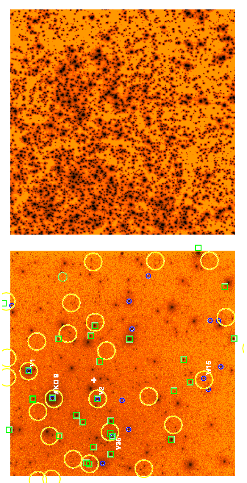
Figure 1:

Figure 2:

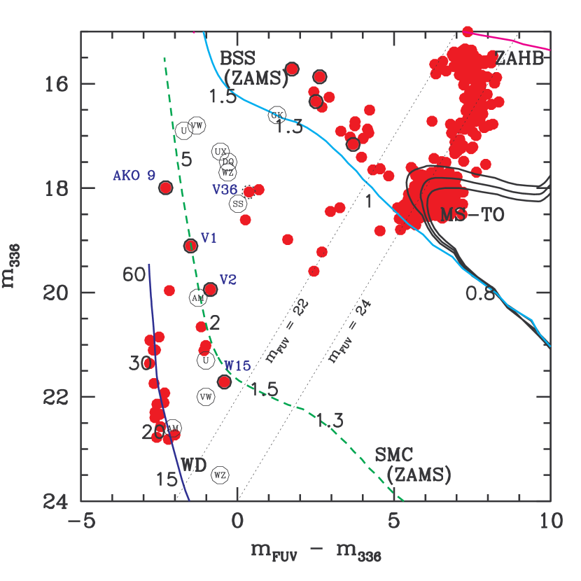
Figure 3:

References

- (1) Albrow, M. D. et al. 2001, ApJ, 559, 1060
- (2) Althaus, L. G. & Benvenuto, O. G. 1998, MNRAS, 296, 206
- (3) Auriére, M., Koch-Miramond, L., & Ortolani, S. 1989, A&A, 214, 113
- (4) Bertin, E. , & Arnout, S. 1996 A&AS, 117, 393
- (5) Böhm-Vitense, E. 1997, AJ, 113, 13
- (6) Bruch, A. & Engel, A. 1994, A&AS, 104, 79
- (7) Cool, A. M., Grindlay, J. E., Cohn, H. N., Lugger, P. M. & Bailyn, C. D. 1998, ApJ, 508, L75
- (8) Davies, M. 1997, MNRAS, 288, 117
- (9) De Marchi, G., Paresce, F. & Ferraro, F. R. 1993, ApJSS, 85, 293
- (10) Di Stefano, R. & Rappaport, S. 1994, ApJ, 423, 274
- (11) Dorman, B. 1992, ApJS, 81, 221
- (12) Fabian, A. C., Pringle, J. E., Rees, M. J. 1975, MNRAS, 172, L15
- (13) Ferraro, F. R., D’Amico, N., Possenti, A., Mignani, R. P. & Paltrinieri, B. 2001, ApJ, 561, 337
- (14) Geffert, M., Auriére, M. & Koch-Miramond, L. 1997, A&A, 327, 137
- (15) Gilliland, R. L., Edmonds, P. D., Petro, L. D., Saha, A. & Shara, M. M. 1995, ApJ, 447, 191
- (16) Grindlay, J. E., Heinke, C., Edmonds, P. D. & Murray, S. S. 2001a, Sci, 292, 2290
- (17) Grindlay, J. E., Heinke, C., Edmonds, P. D., Murray, S. S. & Cool, A. M, 2001b, ApJL, 563, 53
- (18) Guhathakurta, P., Yanny, B., Schneider, D. P. & Bahcall, J. N. 1992, ApJ, 104, 1790
- (19) Harris, W. E. 1996, AJ, 112, 1487
- (20) Howell, J. H., Guhathakurta, P. & Gilliland, R. L. 2000, PASP, 112, 1200
- (21) Hubeny, I., Lanz, T. & Jeffery, C. S. 1994, tlusty and synspec: A User’s Guide, Newsletter on Analysis of Astronomical Spectra (Univ. of St. Andrews)
- (22) Knigge, C., Shara, M. M., Zurek, D. R., Long, K. S. & Gilliland, R. L. 2002, in: “Stellar Collisions, Mergers and their Consequences”, ed. M. M. Shara, ASP Conference Series, Vol. 263, in press (astro-ph/0012187)
- (23) Paresce, F. et al. 1991, Nature, 352, 297
- (24) Renzini, A. & Fusi Pecci, F. 1988, ARA&A, 26, 199
- (25) Richer, H. B. et al. 1997, ApJ, 484, 741
- (26) Robinson, R. D., Carpenter, K. G. & Brown, A. 1998, ApJ, 503, 396
- (27) Stetson, P. 1987, PASP, 99, 191
- (28) Tout, C. A., Pols, O. R., Eggleton, P. P. & Han, Z. 1996, MNRAS, 281, 257
- (29) Valtchanov, I., Pierre, M. & Gastaud, R. 2001, A&A, 370, 689
- (30) VandenBerg, D. A. 2000, ApJS, 129, 315
- (31) van Teeseling, A., Beuermann, K. & Verbunt, F. 1996, A&A, 315, 467
- (32) Vennes, S. et al. 1993, ApJ, 410, L119
- (33) Verbunt, F. & Hasinger, G. 1998, A&A, 336, 895
- (34) Zoccali, M. et al. 2001, ApJ, 553, 733