Optical Gravitational Lensing Experiment. OGLE-1999-BUL-19: The First Multi-Peak Parallax Event

Abstract

We describe a highly unusual microlensing event, OGLE-1999-BUL-19. Unlike most standard microlensing events, this event exhibits multiple peaks in its light curve. The Einstein radius crossing time for this event is approximately one year, which is unusually long. We show that the additional peaks in the light curve can be caused by the very small value for the relative transverse velocity of the lens projected into the observer plane ($\tilde{v}\approx 12.5\pm 1.1{\rm\,km\,s^{-1}}$). Since this value is significantly less than the speed of the Earth’s orbit around the Sun ($v_{\oplus}\sim 30{\rm\,km\,s^{-1}}$), the motion of the Earth induces these multiple peaks in the light curve. This value for $\tilde{v}$ is the lowest velocity so far published and we believe that this is the first multiple-peak parallax event ever observed. We also found that the event can be somewhat better fitted by a rotating binary-source model, although this is to be expected since every parallax microlensing event can be exactly reproduced by a suitable binary-source model. A face-on rotating binary-lens model was also identified, but this provides a significantly worse fit. We conclude that the most-likely cause for this multi-peak behaviour is due to parallax microlensing rather than microlensing by a binary source. However, this event may be exhibiting slight binary-source signatures in addition to these parallax-induced multiple peaks. With spectroscopic observations it is possible to test this ‘parallax plus binary-source’ hypothesis and (in the instance that the hypothesis turns out to be correct) to simultaneously fit both models and obtain a measurement of the lens mass. Furthermore, spectroscopic observations could also supply information regarding the lens properties, possibly providing another avenue for determining the lens mass. We also investigated the nature of the blending for this event, and found that the majority of the $I$-band blending is contributed by a source roughly aligned with the lensed source. This implies that most of the $I$-band blending is caused by light from the lens or a binary companion to the source. However, in the $V$-band, there appears to be a second blended source 0.34 arcseconds away from the lensed source. Hubble Space Telescope observations will be very useful for understanding the nature of the blends. We also suggest that a radial velocity survey of all parallax events will be very useful for further constraining the lensing kinematics and understanding the origins of these events and the excess of long events toward the bulge.

1 Introduction

At the time of writing, more than one thousand microlensing events are known. In addition to the original goal to search for the dark matter (Paczyński 1986), these events have also developed diverse applications (see Paczyński 1996 for a review). Most of these events are well described by the standard shape (e.g., Paczyński 1986). Unfortunately, from these standard microlensing light curves, the lens distance and mass cannot be uniquely determined (see §2). This degeneracy is one of the major obstacles in studies of microlensing.

Fortunately, some microlensing events show deviations from the standard shape. The parallax microlensing events are one class of these exotic microlensing events (Gould 1992). These events allow one to derive the projected Einstein radius (or equivalently, the transverse velocity) in the ecliptic plane. This additional constraint partially lifts the lens degeneracy, but is not enough to uniquely determine the mass of the lensing object; to do this some other piece of information is required, such as the angular Einstein radius. This is a rare occurrence, but a striking example of this can be seen in An et al. (2002), where parallax signatures were observed in a caustic-crossing binary-lens event; this completely broke the lens-mass degeneracy and proved to be one of the first ever measurements of the microlens mass. Alcock et al. (2001a) also claim to have made a determination of the microlens mass for a different event by utilising measurements of both the parallax effect and the microlens proper motion. However, this mass determination relies on their photometric measurement of the parallax effect, which in this instance is very small and requires confirmation (this can be done by obtaining a measurement of the astrometric parallax using HST, for example). Other approaches to this degeneracy problem include resolving the components of the lensed object, which should become possible in the near-future with the availability of suitable optical long baseline interferometry (see Delplancke, Górski & Richichi 2001). However, in the absence of further information the parallax effect can be combined with a model for the lens kinematics, which allows important constraints on the lens to be drawn. So far about 10 microlensing parallax events have been found (Alcock et al. 1995; Mao 1999; Smith, Woźniak & Mao 2002; Bennett et al. 2001; Mao et al. 2002; Bond et al. 2001). Three of these events are particularly interesting (Bennett et al. 2001; Mao et al. 2002) because the long Einstein radius crossing time and the kinematics imply that the lenses are very likely intervening black holes (see also Agol et al. 2002). This is particularly exciting because these black holes may be outside the gas layer of the disk, and hence have no accretion signatures for detection in any other wavelengths such as X-ray and radio. Microlensing may be the only method to provide a complete census of the massive black holes in the Milky Way.

Nearly all of the published microlensing parallax events are identified by a slight asymmetry in the light curve due to the Earth’s motion around the Sun. During the systematic search of Smith et al. (2002), which analysed the 520 microlensing events published in Woźniak et al. (2001), one event has been uncovered that can be very well fitted by the parallax model. This event shows a striking multi-peak signature. Such multi-peak events have been predicted by Gould, Miralda-Escude, & Bahcall (1994). The purpose of this paper is to present a detailed analysis of this event. The outline of the paper is as follows: in Section 2 we present the observational data, the data reduction procedure and our method to select the parallax events from the microlensing database. In Section 3 we present the best parallax model, while in Section 4 we explore whether OGLE-1999-BUL-19 can be fitted by alternate rotating binary-source and binary-lens models. Section 5 discusses the various approaches that can be utilised to provide a measurement of (or strong constraints on) the lens mass. Finally, in Section 6, we summarize and further discuss our results.

2 Observations, Data Reduction and Selection Procedure

The observations presented in this paper were carried out during the second phase of the OGLE experiment with the 1.3 m Warsaw telescope at the Las Campanas Observatory, Chile. The observatory is operated by the Carnegie Institution of Washington. The telescope was equipped with the ‘first generation’ camera with a SITe 2048$\times$2048 pixel CCD detector working in the drift-scan mode. The pixel size was 24$\mu$m, giving the scale of 0.417^′′  per pixel. Observations of the Galactic bulge fields were performed in the ‘medium’ speed reading mode with the gain 7.1 e^- ADU^-1 and readout noise about 6.3 e^-. Details of the instrumentation setup can be found in Udalski, Kubiak & Szymański (1997). The majority of the OGLE-II frames were taken in the I-band, roughly 200-300 frames per field during observing seasons 1997–1999. Udalski et al. (2000) gives full details of the standard OGLE observing techniques, and the DoPhot photometry (Schechter, Mateo & Saha 1993) is available from the OGLE web site.

OGLE-1999-BUL-19 was identified during a search through a catalogue of microlensing events that had been compiled from the three year OGLE-II bulge data. This catalogue, which was generated using the difference image analysis technique, is available electronically and interested readers are referred to Woźniak et al. (2001) and Woźniak (2000) for further details. The aim of the search through this catalogue was to identify potential parallax microlensing events, and the details of this procedure can be found in Smith et al. (2002).

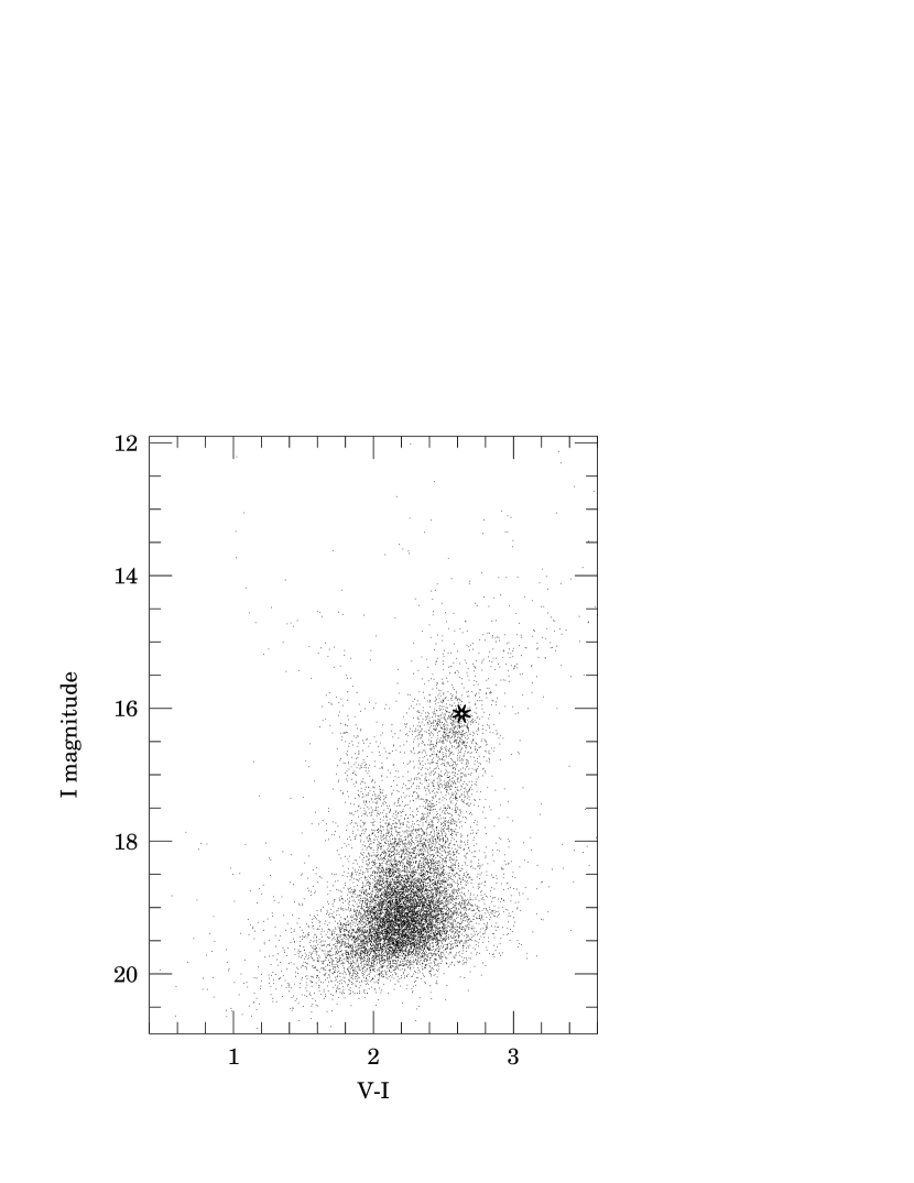
Figure 1: The colour-magnitude diagram of the $5\arcmin\times 5\arcmin$ field around OGLE-1999-BUL-19. The position of OGLE-1999-BUL-19 is marked with an asterisk. The star is located in the red-clump region.

In fact, this event was first detected by the OGLE Early Warning System as OGLE-1999-BUL-19. Throughout this paper we shall refer to this event as OGLE-1999-BUL-19, although in the difference image analysis catalogue of Woźniak et al. (2001) it is labelled sc40_2895. The position of the star is RA=17:51:10.76, and DEC=$-$33:03:44.1 (J2000). The Galactic coordinates are $l=357^{\circ}.077,\>b=-3^{\circ}.147$, and the ecliptic longitude and latitude are $268^{\circ}.126$ and $-9^{\circ}.637$, respectively. The total I-band magnitude of the lensed star plus blend(s) is about $I\approx 16.07$. The average $V-I$ colour of the composite is about $2.63\pm 0.05$. Fig. 1 shows the colour-magnitude diagram for the stars within a field of view $5\arcmin\times 5\arcmin$ around OGLE-1999-BUL-19. From this figure it is clear that the star is located in the red clump region.

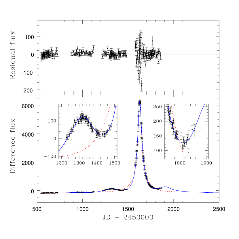
Figure 2: The I-band light curve for OGLE-1999-BUL-19 from difference image analysis, with flux given in units of 10 ADU, which can be converted into magnitudes using the transformation given in §3. The dotted and solid lines are for the best standard and parallax fits, respectively. The insets detail the two unusual bumps in this light curve, clearly showing how successful the parallax model is in fitting these features. The top panel shows the residual flux (the observed data points subtracted by the parallax model). The fact that there are no significant systematic deviations from the horizontal axis indicate the goodness of the parallax fit. The large scatter in the early part of the 4th season of data is explained in §3 of the text.

Initially we analysed just the three season data from 1997 to 1999 (available online; Woźniak et al. 2001). However, we noticed that the parallax model predicts a huge spike in the 2000 season. In order to test this, we subsequently analysed the data from this season. Reassuringly, this confirmed the existence of a huge spike, already seen (but unknown to the modellers) by the OGLE Early Warning System. The four-season data from the difference image analysis are shown in Fig. 2. In total, there are 317 data points in the light curve. In the next section we present both the best standard and parallax model for this unique event, while in §4 we explore the alternate models.

The data for this event can be found online. This site includes the full sequence of $I$-band subframes for this event, the finding chart for the star, the DoPhot photometry, and the full 4-season difference image analysis data that was used to model this event.

3 Standard and Parallax Models

First, OGLE-1999-BUL-19 is fit with the standard single microlens model. In this model the (point) source, the lens and the observer are all assumed to move with constant spatial velocities. The standard light curve, $A(t)$ is given by (e.g., Paczyński 1986):

$$A(t)={u^{2}+2\over u\sqrt{u^{2}+4}},~{}~{}u(t)\equiv\sqrt{u_{0}^{2}+\tau(t)^{2}},$$ (1)

where $u_{0}$ is the impact parameter (in units of the Einstein radius) and

$$\tau(t)={t-t_{0}\over t_{\rm E}},~{}~{}t_{\rm E}={\tilde{r}_{\rm E}\over\tilde{v}},$$ (2)

with $t_{0}$ being the time of the closest approach (i.e., maximum magnification), $\tilde{r}_{\rm E}$ the Einstein radius projected into the observer plane, $\tilde{v}$ the lens transverse velocity relative to the observer-source line of sight, also projected into the observer plane, and $t_{\rm E}$ the Einstein radius crossing time. The Einstein radius projected into the observer plane is given by

$$\tilde{r}_{\rm E}=\sqrt{4GMD_{\rm s}x\over{c^{2}(1-x)}},$$ (3)

where $M$ is the lens mass, $D_{\rm s}$ the distance to the source and $x=D_{\rm l}/D_{\rm s}$ is the ratio of the distance to the lens and the distance to the source. Equations (1-3) show the well-known lens degeneracy in standard microlensing light curves. In this model the only measurable quantity that holds any information about the lens properties is $t_{\rm E}$. This means that for a given value of $t_{\rm E}$ one cannot infer $\tilde{v}$, $M$ and $x$ uniquely, even if the source distance is known.

The flux difference obtained from difference image analysis can be written as

$$f(t)=f_{\rm s}\left[A(t)-1\right]+\Delta f,$$ (4)

where $f_{\rm s}$ is the baseline flux of the lensed source, and $\Delta f\equiv f_{0}-f_{R}$ is the difference between the baseline flux ($f_{0}$) and the flux of the reference image ($f_{R}$). All the fluxes here are in units of 10 ADU and can be converted into $I$-band magnitudes using the transformation given in Woźniak et al. (2001). This value $f_{0}$ is composed of both the baseline flux of the lensed star plus the flux from the lens and/or any unlensed blended star(s), if present. Note that in general $\Delta f$ does not have to be zero or even positive as the reference image can be brighter than the true baseline image ($f_{R}>f_{0}$). For OGLE-1999-BUL-19, the reference image flux is $f_{R}=1048.01$ (Woźniak et al. 2001). To fit this I-band data with the standard model, we need the five parameters given above: $f_{\rm s}$, $\Delta f$ (or $f_{0}$), $u_{0},t_{0}$, and $t_{\rm E}$. Best-fit parameters (and their errors) are found by minimizing the usual $\chi^{2}$ using the MINUIT program in the CERN library.

Table 1: The best standard model (first row) and the best parallax model (second row) for OGLE-1999-BUL-19. The parameters are explained in §3.

Model	$t_{0}$	$t_{\rm E}$ (day)	$u_{0}$	$f_{\rm s}$	$\Delta f$	$\psi$	$\tilde{r}_{\rm E}$ (AU)	$\chi^{2}$/dof
$S$	$1628.146\pm 0.044$	$166.9\pm 1.6$	$0.1075\pm 0.0014$	$783\pm 11$	$-124.66\pm 0.88$	—	—	17912/312
P	$1628.43\pm 0.21$	$372.0\pm 3.3$	$-0.469\pm 0.004$	$706.0_{-8.3}^{+8.4}$	$-188.0\pm 1.1$	$3.1369_{-0.0011}^{+0.0010}$	$2.684_{-0.023}^{+0.024}$	590.1/310

The best-fitting light curve for the standard model is shown by the dotted line in Fig. 2, and the fit parameters are presented in Table 1. Clearly this model comprehensively fails to reproduce the behaviour shown by the data. The $\chi^{2}$ per degree of freedom is greater than 50, and so this model can be discounted unequivocally.

The next logical step is to attempt a fit that incorporates the parallax effect, since the duration of the event is particularly long: as can be seen from the light curve, $t_{\rm E}$ is in the region of a few hundred days, during which time the Earth will have moved substantially in its orbit around the Sun. This invalidates the standard model’s assumption that the observer moves with a constant spatial velocity. The Earth’s centripetal acceleration induces a perturbation on the light curve, and this can become important for events with time-scale greater than a few months. Parallax deviations are expected to be especially prominent for events where the relative transverse velocity of the system is small (i.e., comparable to the Earth’s orbital speed), since this means that the Earth’s orbit has a more significant effect on the trajectory. Another factor that affects the magnitude of the parallax deviations is the size of the Einstein radius projected into the observer plane. This radius determines the length scale on which the magnification is calculated, and so the important quantity is the magnitude of the Earth’s motion relative to this projected Einstein radius. Therefore, if the projected Einstein radius is significantly greater than 1 AU then the Earth’s motion will have less effect than if the projected Einstein radius is comparable to 1 AU.

The description of the parallax effect requires two additional parameters to represent the lens trajectory. We describe the trajectory of the lens in the ecliptic plane, following the natural formalism advocated by Gould (2000), and use the two additional parameters: $\tilde{r}_{\rm E}$, the Einstein radius projected into the observer plane; and $\psi$, an angle in the ecliptic plane describing the orientation of the lens trajectory (given by the angle between the heliocentric ecliptic $x$-axis and the normal to the trajectory). The details of this procedure, including a figure illustrating the geometry of the situation, can be found in Soszyński et al. (2001) and will not be repeated here (see also Alcock et al. 1995; Dominik 1998a). Once these two additional parameters have been determined then the trajectory of the lens in the ecliptic plane is completely determined, allowing a calculation to be made of the separation between the lens and the observer (i.e., the quantity that is analogous to the $u_{0}$ parameter from the standard model). The light curve can then be calculated from this separation.

The standard model’s best-fit values are taken as initial guesses for the parameters $f_{\rm s}$, $\Delta f$, $u_{0},t_{0}$, and $t_{\rm E}$. However, initial values of $\tilde{r}_{\rm E}$ and $\psi$ are arbitrarily chosen for a number of combinations to search for any degeneracy in the parameter space. The best-fitting parameters are again found by minimizing the $\chi^{2}$. Notice that the definitions of $u_{0}$ and $t_{0}$ are slightly different from the standard model: $u_{0}$ now corresponds to the closest approach of the lens trajectory to the Sun in the ecliptic plane, and $t_{0}$ is the time of this closest approach. $u_{0}$ is defined such that the Sun lies on the left-hand side of the lens trajectory for positive values of $u_{0}$. Unlike the standard model, these two parameters no longer have straightforward intuitive meanings because of geometric projections and the parallax effect. For example, the lens trajectory’s closest approach in the ecliptic plane does not, in general, correspond to the closest approach in the lens plane and hence does not match the peak of the light curve.

The inclusion of the parallax effect results in a dramatic reduction in the $\chi^{2}$ value. The new fit has a $\chi^{2}$ value of 590 for 310 degrees of freedom, compared to the standard fit’s value of just under 18000. This improvement can clearly be seen from the light curve plotted in Fig. 2. The standard fit is unable to reproduce the two small bumps on either side of the main peak (shown in the two insets on the bottom panel of Fig. 2), resulting in a wholly unfeasible $\chi^{2}$ value. However, the parallax model has no such difficulties and both bumps are suitably fit.

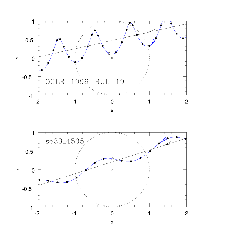
Figure 3: The trajectory of the lens (given by the best-fitting parallax model) in the observer plane relative to the observer-source line-of-sight, i.e., the location of the lens with respect to the Earth (denoted by the small cross). The top panel depicts the trajectory for OGLE-1999-BUL-19, whilst the bottom panel shows a more typical parallax event, sc33_4505 (see §3 and Smith et al. 2002). This separation between the lens and the Earth corresponds to the $u$ value given in eq. (1) and determines the magnification for the event. The straight dashed line represents the equivalent trajectory without accounting for the orbital motion of the Earth (i.e., a standard ‘constant-velocity’ light curve). It should be noted that this does not necessarily correspond to the best-fit standard light curve given in Fig. 2 and Table 1. The solid dots indicate the lens position at 50 day intervals, and the open dots correspond to the approximate peak times, i.e., $t=1650$ and $t=650$ days for OGLE-1999-BUL-19 and sc33_4505, respectively. The large dotted circle represents the size of the event’s Einstein radius, and the axes are given in units of this Einstein radius. For both events the lens traverses from right to left, as depicted by the arrows. This figure demonstrates that the trajectory in the case of event OGLE-1999-BUL-19 is highly non-linear, leading to the exceptionally dramatic parallax signature. Comparing this to a more typical parallax microlensing event, sc33_4505, highlights the spectacular nature of the trajectory for OGLE-1999-BUL-19.

The accuracy of the parallax fit is highlighted in the top panel of Fig. 2, which shows the difference between the data points and the parallax model. Any problems with the parallax fit would manifest themselves as systematic deviations from the horizontal axis; apart from a slight under-prediction of the flux in the second season, the flux consistently matches the value predicted by the parallax model. This $\chi^{2}$ value of 590 for the parallax fit corresponds to a $\chi^{2}$ per degree of freedom of 1.90, a formally unacceptable value. However, from the top panel of Fig. 2 it is clear that most of the excess scatter occurs near the beginning of the fourth season, when the source flux was strongly magnified. Obviously, the Poisson photon noise expressed in counts should rise as the square root of the magnified flux. However, there are also additional sources of noise for brighter stars in most ground based CCD imaging. Most of these effects in OGLE-II data are accounted for by a simple rescaling of the error bars (Fig. 3 in Woźniak 2000). Near the peak of the event at $I\approx 13.8$ magnitudes, the r.m.s. scatter is about 1% in the present data, fully consistent with the scatter for other comparably bright objects in this field. The problem is that the average scaling curve for all fields may not fully reflect the photometric uncertainty for bright stars in this part of the BUL_SC40 field. The error bars may be under-estimated in this region which then result in an artificially large $\chi^{2}$ value. A possible explanation might be the larger than average extinction in this field, contributing to lower signal to noise in the fitted kernels and point spread functions. To ensure that these observed systematics are not an artifact of our method of photometric data reduction (i.e., difference image analysis), we made a parallax fit to the regular photometry obtained with DoPhot. The corresponding residual plot, when converted from magnitudes into counts, shows all the same features that have been discussed above, but with a marginally larger overall scatter. Therefore the following analysis is based solely on the difference image analysis data.

The model parameters for the best-fitting parallax model are presented in Table 1. It can be seen from this table that all of the parameters, and most notably the ones describing the lens trajectory ($u_{0}$ and $\psi$), are very tightly constrained, due to the fact that the parallax deviations are especially pronounced. Another aspect of the light curve that probably contributed to the tightly-constrained nature of the parameters was the brightness of the event, since this reduces the size of the photometric error bars. The total I-band baseline magnitude for this event is approximately 16.07 magnitudes, and the parallax model predicts that the lensed star contributes 82 percent of this, i.e., there is only slight blending and the baseline magnitude of the lensed star alone is 16.3 magnitudes. The lensed star was also quite strongly magnified at the peak, rising to a magnification of greater than 10 ($A_{\rm max}\approx 10.2$).

The parameters that help in determining the lens properties are:

$$\tilde{r}_{\rm E}=2.68\pm 0.23\,{\rm AU},~{}~{}t_{\rm E}=372.0\pm 3.3\,{\rm day},~{}~{}$$ (5)

From these an expression for the lens mass can be determined, although due to the degeneracy inherent in the microlensing light curve this can only be expressed as a function of the relative lens-source distance (see Soszyński et al. 2001; Gould 2000),

$$M=\frac{c^{2}\tilde{r}_{\rm E}^{2}}{4G}\left({{1\over D_{\rm l}}-{1\over D_{\rm s}}}\right)=0.088M_{\odot}\left(\frac{\tilde{r}_{\rm E}}{\rm 2.68\,AU}\right)^{2}\left(\frac{\pi_{\rm rel}}{0.1\rm mas}\right),~{}~{}\pi_{\rm rel}\equiv{{{\rm AU}\over D_{\rm l}}-{{\rm AU}\over D_{\rm s}}}.$$ (6)

As can be seen from this equation, the lens mass depends on the relative lens-source parallax, $\pi_{\rm rel}$. Fig. 1 suggests that the star is a red-clump star in the bulge, so its distance is approximately 8 kpc. If the lens is lying half-way in-between (i.e., $D_{\rm s}\approx 8\,$kpc and $D_{l}\approx 4\,$kpc), then $\pi_{\rm rel}=0.125\,{\rm mas}$, and this would imply a lens mass of around $0.11M_{\odot}$. However, if the lens is very close to us, say $D_{\rm l}\sim 550$ pc (which corresponds to $\pi_{\rm rel}>1.6\rm mas$), then this lens mass can be as large as $1.4M_{\odot}$.

The value of the transverse velocity projected into the observer plane suffers from no such degeneracy and can be determined uniquely,

$$\tilde{v}=\frac{\tilde{r}_{\rm E}}{t_{\rm E}}=12.5\pm 1.1\mbox{ km s}^{-1}.$$ (7)

This velocity is exceptional in that it is the lowest ever recorded for a published parallax microlensing event. Possible causes for such a low velocity are discussed in §6.

The exaggerated nature of the parallax signatures can be accounted for when it is noted that the projected lens velocity, $\tilde{v}$, is much less than the orbital speed of the Earth ($v_{\oplus}\approx 30\mbox{ km s}^{-1}$). Because of this, as the lens trajectory passes the Earth the change in separation is dominated by the motion of the Earth, rather than the motion of the lens as in normal microlensing events. The trajectory of the lens relative to the observer-source line of sight is shown in the top panel of Fig. 3, and the highly non-linear nature can clearly be seen. During the 6 months before the point of closest approach the Earth swung away from the lens and increased the separation, with the maximum separation occurring at around 1450 days. This can be contrasted with the behaviour during the 6 months directly preceding this region (i.e., approximately $1250<t\equiv{\rm JD}-2450000<1450$ days), where the Earth completed another half-orbit and its trajectory brought it back towards the lens. These two regions correspond, respectively, to the unusual declining and rising sections of the light curve which occur before the main peak, i.e., the parallax induced ‘bump’ at around $t=1300$ days. Similarly, this behaviour is repeated in the 12 months following the point of closest approach: during the 6 months directly following the point of closest approach the Earth moves away from the lens, resulting in a sharp decline in flux; however, in the subsequent 6 month period the Earth begins to move back toward the lens resulting in a sharp rise in flux. This period of one year, from approximately $t=1650$ to $t=2000$ days, corresponds to the trough around $t=1800$ days.

The highly unusual nature of this event is highlighted when its trajectory is compared to that of another, more typical, parallax affected light curve. The bottom panel of Fig. 3 shows the trajectory for the microlensing event sc33_4505 which was discovered during the parallax search through the OGLE-II database of microlensing events toward the galactic bulge (see Smith et al. 2002). This event had unexceptional values of $\tilde{r}_{\rm E}$ and $\tilde{v}$ (6.37 AU and $57\,\mbox{kms}^{-1}$ respectively), and the corresponding trajectory can be seen in Fig. 3 to be much closer to the standard linear approximation than for OGLE-1999-BUL-19. This is because the velocity of the lens is about twice the size of the Earth’s velocity; in the time that it takes the lens to cross its projected Einstein diameter the Earth has completed approximately one orbit, whereas for OGLE-1999-BUL-19 the Earth completes nearly two orbits in this time. Another factor that leads to the parallax effect being more pronounced in OGLE-1999-BUL-19 is that the value of the projected Einstein radius, $\tilde{r}_{\rm E}$, is much smaller than for sc33_4505. This effect has been discussed above, and its influence can clearly be seen in Fig. 3.

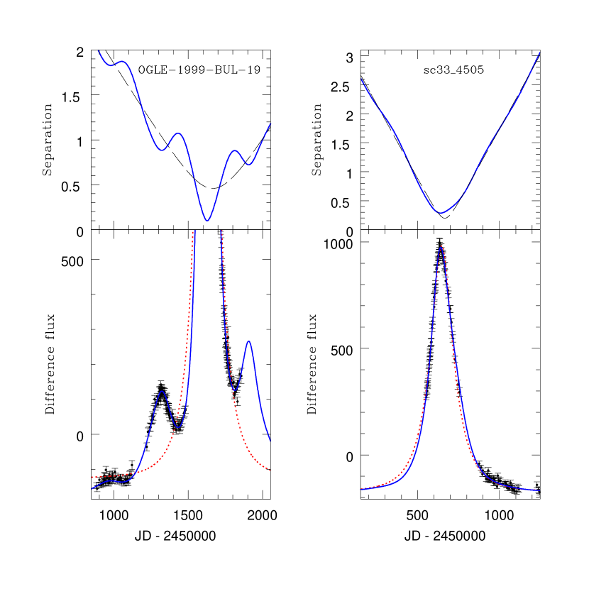
Figure 4: The magnitude of the separation (given by the best-fitting parallax model) between the lens and the observer-source line-of-sight (top panel), and how this relates to the light curve (bottom panel), for OGLE-1999-BUL-19 (left) and a more typical parallax microlensing event sc33_4505 (right; see §3 and Smith et al. 2002). In the top panels the separation determined from the parallax fit is given as a solid line, and the dashed line represents how this separation would look without the orbital motion of the Earth (i.e., a standard ‘constant-velocity’ light curve). The separation, which is in units of the Einstein radius, corresponds to the $u$ value given in eq. (1) and determines the magnification for the event. The lower panels show the I-band light curve for each event, with the dotted and solid lines corresponding to the best-fit standard and parallax models, respectively. This figure demonstrates the highly non-linear nature of the trajectory for event OGLE-1999-BUL-19, as can be seen from the significant deviations in separation between the parallax trajectory and the standard-type trajectory. These deviations are clearly much more prominent in the separation plot of OGLE-1999-BUL-19, compared to sc33_4505. From this plot one can easily identify the origins of the irregular bumps in the light curve of event OGLE-1999-BUL-19, which correspond to the separation minima in the upper panel. Note that the dashed line in the top panel does not necessarily correspond to the best-fitting standard model given in the lower panel - this is included solely to give an indication of the deviation of the parallax separation from a linear trajectory.

Since the magnification is dependent on the magnitude of the separation of the lens from the observer-source line of sight, a plot of how this separation varies with time is helpful to elucidate the situation. This is shown in Fig. 4. The separation for the OGLE-1999-BUL-19 event (given in the upper-left panel) clearly varies significantly from the hyperbolic shape of a standard microlensing light curve (shown as a dashed line); the Earth’s orbital motion induces an annual oscillation onto this standard hyperbolic form, and from this oscillation one can unmistakably identify the origins of the two additional parallax bumps. However, the situation is much less clear for the sc33_4505 event; the oscillations are much smoother and much smaller in magnitude. The origins of the additional peaks and troughs in the light curve of OGLE-1999-BUL-19 can easily be identified from this figure, since they obviously correspond to the points at which the rate of change of separation, $\dot{u}$, is zero. For a typical microlensing event $\dot{u}=0$ only occurs once at the point of closest approach. However, when the projected lens velocity is so low, as is the case in OGLE-1999-BUL-19, the motion of the Earth can cause there to be additional local points of closest approach, in addition to the global point of closest approach.

4 Alternate Models

4.1 Binary-source model

It is necessary to test whether this unusual behaviour could be caused by any other phenomena, such as a rotating binary source or binary lens. In fact, the OGLE Early Warning System initially identified this event as a binary-source event. To address this we first fit OGLE-1999-BUL-19 with a rotating binary-source model (using a method similar to that of Dominik 1998a; see also Griest & Hu 1992). However, to simplify the process, only circular orbits are considered initially. The generalization to elliptical orbits is considered later in §4.1.2. Both models are described in detail in the appendix.

4.1.1 Circular orbits

A total of 12 parameters are required to describe this circular rotating binary-source model, i.e., a further 7 parameters in addition to the 5 from the standard model. The motion of the two sources are described using the following parameters: the period of the orbit, $T$; the binary-source separation, $p$, which is given in units of the Einstein radius projected into the source plane; the flux ratio of the first source, ${\cal F}$, i.e., ${\cal F}=\frac{f^{(1)}}{f^{(1)}+f^{(2)}}$ where $f^{(1)}$ and $f^{(2)}$ are the fluxes from the first and second source, respectively; and the mass fraction of the first source, ${\cal M}$, i.e., ${\cal M}=\frac{m^{(1)}}{m^{(1)}+m^{(2)}}$ where $m^{(1)}$ and $m^{(2)}$ are the masses of the first and second source, respectively. As well as these parameters, a further three angles are required: two, $\alpha$ and $\beta$, to determine the orientation of the orbital plane; and an angle to describe the lens trajectory in the orbital plane, $\Theta$. Once the above 7 parameters have been combined with those from the standard model (i.e., $t_{0}$, $t_{E}$, $u_{0}$, $f_{\rm s}$, $\Delta f$) then the light curve can be calculated. It should be noted that only the flux and mass ratios (directly) enter our parametrization, not the individual fluxes and masses of each source. A complete description of this model, including the procedures for calculating the light curve, is given in the appendix A1 and will not be repeated here.

As before, the best-fit parameters are found by minimizing the $\chi^{2}$. However, since the description of this model requires a large number of parameters, the $\chi^{2}$ surface is very intricate. This presents a problem when attempting to find the global minimum, and to address this issue the initial guesses for the parameters are chosen from a large set of randomly generated values. In this analysis the parameter space is not searched exhaustively and although a range of fits were found with comparable $\chi^{2}$ values, only the single best-fit set of parameter values is considered.

Table 2: The best-fit parameters for the circular binary-source model. The parameters are explained in §4.1 and in the appendix (§A1). The errors have been omitted since they were found to be misleading, owing to the complexity of the $\chi^{2}$ surface.

$t_{0}$	$t_{\rm E}$ (day)	$u_{0}$	$f_{\rm s}$	$\Delta f$	$\alpha$	$\beta$
$1628.8$	$408$	$-0.43$	$609$	$-191$	$-1.65$	$6.14$
$T$ (day)	$p$	${\cal F}$	${\cal M}$	$\Theta$	$\chi^{2}$	dof
$368$	$2.0$	$0.0003$	$0.169$	$4.60$	545.20	305

The parameter values corresponding to the best-fit model are presented in Table 2. The errors have been omitted since they were found to be misleading, owing to the complexity of the $\chi^{2}$ surface. It is expected that the best-fit binary-source model should, at least, provide a fit that is comparable to the best-fit parallax model; this is because a binary-source model can always be found that is the exact mirror-image of the parallax model, i.e., a fit which has all of the flux coming from one single source (${\cal F}=0\;\mbox{or}\>1$) , an orbital period of one year, etc. It should be noted that this is a generic property of any parallax microlensing event where the parallax and binary-source models are fitted independently. However, for this event the best-fit binary-source $\chi^{2}$ value is 545.2 (or 1.79 per degree of freedom), which is a distinct improvement on the best-fit parallax value of 590.1 (or 1.90 per degree of freedom).

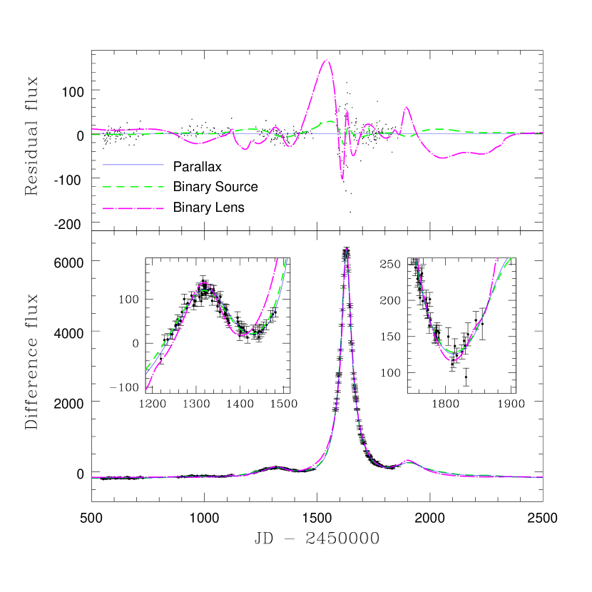
Figure 5: A diagram to compare the two best-fit binary models with the best-fit parallax model. The bottom panel shows the usual I-band light curve, with the best parallax model given by the solid line, the best rotating circular binary-source model given by the dashed line, and the best face-on rotating binary-lens model given by the dot-dashed line. The insets detail the two unusual bumps in this light curve. Notice that the binary-lens model does not match the first two season data well. The top panel shows the residual flux (the observed data points subtracted by the parallax model). This figure shows how closely the binary-source light curve matches the parallax light curve, with the slight differences only becoming apparent in the residual plot.

Fig. 5 shows the light curve for this fit, and for comparison the best-fit parallax light curve is also included. The minute differences between the two fits are only discernible in the top panel of Fig. 5. This panel shows the difference between the data points and the parallax model, along with the predicted binary-source flux. Clearly the two fits exhibit only slight discrepancies, with the largest digression occurring during the early part of the fourth season, i.e., during the period where the error bars in the data may be unreliable (see §3).

However, a closer inspection of the best-fit parameters shows that whilst this model may result in an improvement in the $\chi^{2}$ value, it could indeed be a reproduction of the best-fit parallax model. This deduction is made because of two parameter values in particular: the binary period, $T$, and the flux ratio, ${\cal F}$. The period of this binary orbit is approximately $368$ days, which is suspiciously close to the period of the Earth’s orbit. In addition, the flux ratio is practically zero, which implies that all of the flux is coming from just one of the sources, i.e., analogous to the parallax model.

Further evidence can be found by analysing the other parameters; for example, it can be shown that the orientation of the orbital plane is almost identical to the orientation of the ecliptic plane in the parallax model. Similar comparisons can made for the trajectory of the lens, the radius of the orbit and the impact parameter. From this we conclude that the best-fit binary-source model is simply a reproduction of the best-fit parallax model. However, this does not explain why there should be such a large improvement in $\chi^{2}$ between the parallax and binary-source models. This issue is dealt with later, in §5.1.

If the source is a red clump star located in the bulge (as is indicated by Fig. 1), then its apparent magnitude and colour can be estimated to be $I_{\rm s}\approx 14.15$ and $(V-I)_{\rm s}\approx 1.19$ (see §5.3). The star’s colour is roughly consistent with theoretical predictions for clump giants of mass $M\approx 1\,M_{\odot}$ with solar metallicity and age 5-12 Gyr (Table 1 in Girardi & Salaris 2001). If we assume that the source is 7 to 8 kpc away from the source, then its absolute magnitude is also consistent with the theoretical prediction (see also Fig. 14 in Girardi & Salaris 2001). If the source mass is assumed to be $M_{\rm s}\approx 1\,M_{\odot}$, this can be combined with an estimate of the source distance ($D_{\rm s}\approx 8\,\rm{kpc}$) to obtain a prediction for the separation and radial velocity of the above binary. Using Kepler’s law, the separation of the two sources is approximately, $a=\left[\frac{{\rm G}}{4\pi^{2}}\frac{M_{\rm s}}{1-{\cal M}}T^{2}\right]^{1/3}=1.07\,\rm{AU}$, and the radial velocity variations should have a semi-amplitude of around $5.3\,\rm{kms}^{-1}$ with a period 368 days. Since $p$ is the binary source separation in terms of the Einstein radius projected into the source plane, i.e., $p=a/(D_{\rm s}\theta_{E})$, we can therefore estimate the size of the angular Einstein radius,

$$\theta_{\rm E}=\frac{{a}}{p}\times\frac{1}{D_{\rm s}}\approx 65\mu\rm{as}.$$ (8)

This value of $\theta_{\rm E}$ is very small, and it may be in contradiction with later limits on $\theta_{\rm E}$ estimated from finite source size considerations (see §5.3 and discussion).

4.1.2 Elliptical orbits

Since the best-fit binary-source parameters predict that the flux ratio is almost exactly zero, we proceeded to analyse fits which have this flux ratio set to 0, implying that all the flux comes from one of the sources. Because of this condition there is now a degeneracy between $p$ and ${\cal M}$, and only the product of these two parameters is physically meaningful ($p\,{\cal M}$ is now the orbital semi-major axis for the luminous source). We choose to set ${\cal M}=1$, which means that $p$ now corresponds to the orbital semi-major axis for the luminous source.

As there are now two fewer parameters, it becomes more feasible to fit for elliptical orbits. This introduces two additional parameters: the eccentricity, $e$; and the phase of the orbit, $\xi_{0}$. The details of this model can be found in the appendix (§A.2). If this model is to reproduce a mirror-image of the parallax model (as discussed above), then we would expect the eccentricity, $e$, to be close to zero, resulting in a near-circular orbit. This is because, unlike the Earth’s orbit (which has $e_{\oplus}\sim 0.017$), it is rare for binary stars to have nearly circular orbits (Duquennoy & Mayor 1991).

As with the circular binary-source model, the best fit parameters are found by minimizing the $\chi^{2}$. A number of initial guesses were chosen as input parameters, and the single best-fit set of parameters are presented in Table 3.

Table 3: The best-fit parameters for the elliptical binary-source model, with ${\cal M}$ fixed at 1 and ${\cal F}$ fixed at 0. The parameters are explained in §4.1 and in the appendix (§A1 and §A2). The errors have been omitted since they were found to be misleading, owing to the complexity of the $\chi^{2}$ surface.

$t_{0}$	$t_{\rm E}$ (day)	$u_{0}$	$f_{\rm s}$	$\Delta f$	$\alpha$	$\beta$	$T$ (day)
$1627.8$	$428$	$-0.41$	$557$	$-193$	$-4.35$	$0.12$	$367$
$e$	$p$	$\xi_{0}$	${\cal F}$ (fixed)	${\cal M}$ (fixed)	$\Theta$	$\chi^{2}$	dof
$0.010$	$0.32912$	$3.56$	$0$	$1$	$-1.24$	544.84	305

This best-fit provides a slight improvement in the $\chi^{2}$ value compared to the circular binary-source model. However, as can be seen from Table 3, the eccentricity is very close to Earth’s value, and the orbital period is almost exactly one year. Therefore we conclude that this result strengthens the argument that the binary-source model is simply reproducing a mirror-image of the parallax model.

4.2 Binary-lens model

In the previous subsections, we have fitted the light curve of OGLE-1999-BUL-19 with a parallax model and a rotating binary-source model. In this section, we will explore whether OGLE-1999-BUL-19 can be fitted by a rotating binary-lens model.

While the light curves produced by the binary-source or the parallax models are always smooth, those produced by binary lenses may contain sharp rises and falls due to caustic crossings (e.g., Mao & Paczyński 1991). As a result of these new features, the $\chi^{2}$ surface in the multi-dimensional space is even more complex, and it is often difficult to locate the global minimum. Furthermore, for weak binaries and ill-sampled light curves, the solutions are known to be degenerate (Mao & di Stefano 1995; Dominik 1999). For OGLE-1999-BUL-19, the multi-peak behavior is reminiscent of periodic rotations; we have therefore implemented a simple version of rotating binaries (Dominik 1998a) where we assume the binary orbit is face-on, i.e., the orbital plane is perpendicular to the line of sight. Other than the five parameters in the standard model, we have six more parameters that describe the binary and the source trajectory: the binary lens major axis, $p$; the angle, $\phi$, between the normal to the source trajectory and the line connecting the lenses at the time of the perihelion; the period of the binary orbit, $T$; the eccentricity, $\epsilon$; the time of the perihelion, $t_{\rm Peri}$; and the mass ratio ${\cal M}=\frac{m^{(1)}}{m^{(1)}+m^{(2)}}$ where $m^{(1)}$ and $m^{(2)}$ are the masses of the first and second lenses respectively. Note that $t_{\rm E}$ corresponds to the Einstein radius crossing time for the total mass. In total, we have 11 parameters even for this simple face-on rotating binary model.

We have searched for the best fit face-on rotating binary starting from a number of initial guesses (although no exhaustive searches were performed). Fig. 5 shows the best fit which was found. The total $\chi^{2}$ is 1522.4. The parameters are given in Table 4.

Table 4: The best-fit parameters for the face-on rotating binary-lens model. The parameters are explained in §4.2. The errors have been omitted due to the complexity of the $\chi^{2}$ surface.

$t_{0}$	$t_{\rm E}$ (day)	$u_{0}$	$f_{\rm s}$	$\Delta f$	${\cal M}$	$p$
$1536.1$	$230.2$	$-0.536$	$1048.0$	$-168.4$	$0.027$	$0.39$
$\phi$	$T$ (day)	$\epsilon$	$t_{\rm Peri}$		$\chi^{2}$	dof
$1.74$	$463.3$	$0.26$	$1368.5$		1522.4	306

The $\chi^{2}$ is much worse than the best parallax model and binary-source model. Much of the $\chi^{2}$ actually arises from the failure of the binary-lens model to fit the first and second season data. This binary-lens model seems to resemble the observed shape of the light curve, in particular the shape around the peak. However, it does not match the data points for the first three seasons, including the baseline. Note that in this model the lensed source contributes all of the light.

Clearly this fit is not acceptable. It is possible, however, that an improved fit may be found from a more exhaustive search, especially when non-face-on orbits and blending are also considered.

5 Constraints on the Lensing Configuration

5.1 Combined binary-source model incorporating parallax effect

As can be seen from §4, the rotating binary-source model provides the best fit for OGLE-1999-BUL-19. However, it was shown that this model is almost certainly a mirror-image of the best-fit parallax model, and hence not a genuine physical solution. On the other hand, the improvement in $\chi^{2}$ is significant; if the error bars are rescaled so that the $\chi^{2}$ per degree of freedom is 1.0 for the best-fit parallax model, then this corresponds to $\Delta\chi^{2}=23.7$ for an additional 5 degrees of freedom. Obviously this is a significant improvement, and the probability of such an improvement occurring by chance is much less than 1 percent.

This may be accounted for by the additional parameters in the binary-source model; an improved fit can result from a fine-tuning of these additional parameters which are fixed in the parallax model, e.g., orbital period or the orientation of the orbital plane. Another possible explanation for this could be that there are systematic errors in the data, correlated on long time-scales, which are better fit by this rotating binary-source model.

However, a more-likely possibility is that this event is simultaneously exhibiting both parallax and rotating binary-source behaviour. This conclusion can be justified when one considers that the duration of the event is significantly greater than one year, and therefore there must be some parallax effect on the light curve. Hence the simple rotating binary-source fit in §4, which did not incorporate the parallax motion of the Earth, is obviously deficient.

Fitting the data with both the parallax and binary-source models simultaneously would enable constraints to be put on the lens mass. With follow-up spectroscopic observations, a rotating binary-source fit can provide a measurement of, or at least strong constraints on the Einstein radius projected into the source plane, $D_{\rm s}\,\theta_{\rm E}$ (Han & Gould 1997). When combined with the value of $\tilde{r}_{\rm E}$ obtained from the parallax effect, this allows one to measure or constrain $D_{\rm s}\,M$, where $M$ is the lens mass. Since $D_{\rm s}$ is known to be approximately 8 kpc for OGLE-1999-BUL-19, this would at least provide strong constraints on the lens mass for this event, and possibly a direct measurement.

However, the task of fitting the data with both parallax and rotating binary-source models simultaneously is not an easy one. This situation would be helped if the period, phase and eccentricity of the binary orbit could be determined. This can be done through radial velocity measurements of the source, and once these are obtained then they could be incorporated into the fitting procedure to significantly reduce the number of free parameters. Since the Earth’s orbit is known, this means that incorporating the binary-source motion into the parallax model should be feasible, allowing (the aforementioned) tight constraints to be put on the lens mass.

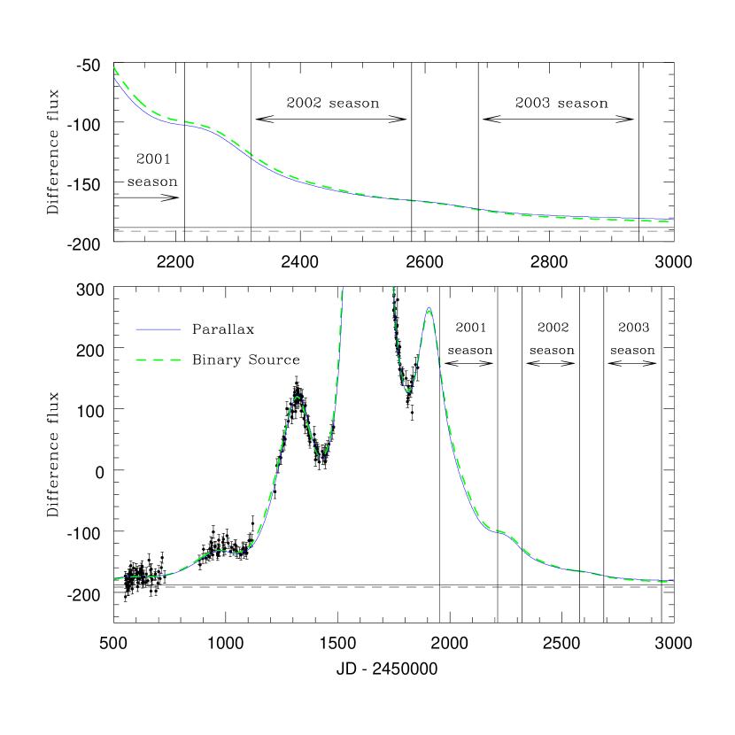
Figure 7: The I-band light curve for OGLE-1999-BUL-19 showing the predicted behaviour for the present and future observing seasons. The solid and dashed lines correspond to the best-fit parallax and circular binary-source models, respectively, and each model’s predicted baseline is also given. The approximate Galactic bulge observing seasons are denoted by vertical lines. Unfortunately, as can be seen from this figure, the final additional peak at $t\approx 1900$ occurred during the break between observing seasons. In addition, it should be noted that there were no OGLE observations during the 2001 season, although data has been gathered by the PLANET collaboration for the latter part of this season (see §6). The top panel details the predicted flux, and from this it is clear that the differences between the binary-source fit and the parallax fit are unlikely to be resolved. However, from this prediction one should be able to test whether the parallax and binary-source models are feasible or not, since they both predict a significant drop in flux between the end of the 2001 season and the beginning of the 2002 season.

So far, very few binary-source microlensing events have been detected (Alcock et al. 2001b, Becker 2000). This is contrary to expectation since many stars in the galaxy are in binaries (Griest & Hu 1992, Dominik 1998b, Han & Jeong 1998). In particular, the progenitor of the source for OGLE-1999-BUL-19 was probably a G-type star on the main sequence with a mass $\approx 1\,M_{\odot}$ (e.g., Table 15.8 from Cox 2000), and it is known that the majority of G-type stars exist in binaries. One explanation for the lack of observed binary-source events is that to be detectable they must have both an impact parameter which is comparable to the binary separation, and also an orbital period which is comparable to the event’s duration, $t_{\rm E}$. Typically, $t_{\rm E}$ is less than a month, and there are very few binary systems which have such short periods. However, event OGLE-1999-BUL-19 has a duration of $t_{\rm E}\approx 370$ days, which could feasibly be comparable to the orbital period of a binary source. Even if the binary period is much greater than 370 days, deviations from the parallax-only fit could still be detectable in this light curve since the microlensing amplification lasts for well over six years in total (as can be seen from Fig. 7). In addition, the source for OGLE-1999-BUL-19 is particularly bright and the parallax fit is well constrained. These two factors should increase the possibility of detecting slight deviations from the predicted parallax-only fit, even if the period is greater than one year. If such deviations are not apparent in the data already obtained, then they may still be observed in the future light curve, especially with improved photometric accuracy.

As well as the above approaches, the astrometric signature may be able to detect the presence of a binary source. The astrometric microlensing signature for an event lasts much longer than its photometric counterpart (e.g., Hosokawa et al. 1993; H${\rm\o}$g, Novikov & Polnarev 1995; Miyamoto & Yoshi 1995; Walker 1995; Paczyński 1998), and could therefore be used to make future observations. As was shown in Han (2001), the astrometric signature for a binary-source microlensing event differs from that of a single-source event, particularly when the binary-source separation is small enough to be detectable in the photometric light curve, as may be the case with OGLE-1999-BUL-19. Therefore, if the parallax and binary-source signatures can be dis-entangled, then this could provide another method of determining the lens mass. However, even if the binary-source signature is not detectable in the astrometric observations, it is still possible to measure $\theta_{\rm E}$ using a single-source fit to the astrometric data and hence constrain the lens mass.

5.2 The nature of the blend(s)

In order to select variable sources, such as microlensing events, the difference image analysis technique automatically subtracts out non-varying sources. However, information on the (non-varying) blended light is also encoded in the images and can be important for understanding the lensing geometry. Gould & An (2002) showed that using a proper linear weighting of the images, one can form an image that is free of the lensed source. In their method, the weighting of the images uses the magnification as a function of time and the frames are convolved to the worst seeing among all frames in the stack. In our case, we took the magnification history from the best parallax model and constructed corresponding images of the lensed source and separately the blended light from neighbouring objects.

For the present application, we are particularly interested in comparing the colours and astrometry of the blend(s) compared with those of the lensed source. If the blended light and the lensed source are not co-aligned, then the star which is causing this blending cannot have any influence on the microlensing event. However, if the blended light is co-aligned with the lensed source, then there are two very interesting possibilities. One is that the light is from the lens itself and the other is that the light is from a (close) binary companion source.

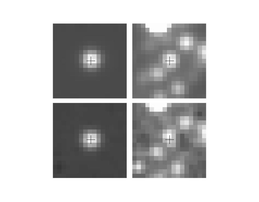
Figure 6: $I$-band (top) and $V$-band (bottom) images for the lensed source (left-panel) and the blended light (right-panel). The crosses indicate the position of the lensed source in each panel. Each pixel in the panels corresponds to 0.417″. East is to the right and north is up.

We applied the Gould & An (2002) method to OGLE-1999-BUL-19. We first analysed the $I$-band images. A reference image was created by stacking the $\sim 80$ best-seeing images. This exercise was somewhat complicated by twelve bad columns close to the lensed star. Fig. 6 shows an $I$-band image of the lensed source (top left) and an $I$-band image of the blend(s), i.e., with the lensed star subtracted (top right). The $I$-band position of the lensed star is indicated by a cross in all images.

From the figure it is clear that in the $I$-band the lensed star and the blend are almost aligned. We used the DoPhot program to obtain the photometry and astrometry of the lensed star and the blend. We found that the lensed source and the blend are co-aligned to within 0.095 pixels (one pixel corresponds to about 0.417 arcseconds for the OGLE-II CCD camera). This offset is within the uncertainty of the OGLE-II astrometry, $\sim 0.05-0.1$ pixels. The blend contributes about 24% of the total flux, which is comparable to but smaller than the value predicted by the parallax model ($\sim 18\%$, see §3). However, we do not regard this discrepancy as very significant given the fact that the image with the lensed source removed is still very crowded. Also, the fact that there may be two unresolved blends (see below) may have noticeably affected the DoPhot photometry. Additional possible uncertainties may arise from correlated noise introduced by convolutions.

Next, we applied the same procedure to the $V$-band images. Most of frames for OGLE-II were taken in the $I$-band, so only 9 $V$-band images are available. We chose 5 frames as the other four have substantially worse seeings. The selected $V$-band frames had slightly better seeing than the typical $I$-band images. Fig. 6 shows the $V$-band images of the lensed source (bottom left) and the blended light (bottom right). In this case, the blended light shows a clear offset. Quantitatively, the blend is about 0.35 pixels to the east, and 0.75 pixels north of the lensed source; it contributes about 27% of the total flux in the $V$-band. This astrometric offset is highly significant statistically. So while in the $I$-band the blended light seems to be aligned with the lensed source, in the $V$-band the blended light seems to show a substantial offset. To verify this, we examined the centroid position of the composite as a function of magnification. The centroid is expected to shift toward the lensed source as its magnification increases (for an example see Alard, Mao & Guibert 1994). This trend is clearly seen in the $V$-band data, whilst it is absent in the $I$-band within the astrometric uncertainties. We note that the combined colour of the blend is similar to the composite as the light fractions contributed by the blends are similar in the $V$-band and in the $I$-band, a fact that we will use in §5.3.

The most straightforward interpretation is that there are actually two blended sources within the seeing disk of the lensed source. One is aligned with the lensed source, and is bright in the $I$-band but faint in the $V$-band, while the other is offset from the lensed source and is bright in the $V$-band but faint in the $I$-band. The $V$-band image actually shows a faint extension, or a wing, of the blend image towards the position of the lensed source, supporting our conclusion about the presence of a second blended source, roughly co-aligned with the lensed source. The spatial resolution from the ground is not sufficient to accurately determine the colours and positions of these two blended sources. HST and ground-based spectroscopy may be important for understanding the nature of the blending; we return to this in the discussion.

If it is assumed that this $I$-band blend is indeed caused by the lens, then it is possible to estimate the properties of the lens using a mass-luminosity relationship. This assumption would give a lens brightness of $I_{\rm l}\approx 17.9$ mag, and from the range of inferred lens masses one can deduce that this would have to be main-sequence star. Therefore, by comparing this luminosity (after extinction has been taken into account) with a mass-luminosity relationship for main-sequence stars (e.g. Cox 2000), it can be shown that the lens would probably be an early M-type or a late K-type dwarf with a mass of around $0.6~{}M_{\odot}$ lying approximately 1.3 kpc from us. This would imply $\theta_{\rm E}\sim 1.7$ mas, which is vastly different from the value calculated from the ‘pure’ binary-source model in §4.1.1 ($\theta_{\rm E}\approx 65\mu\rm{as}$).

5.3 Finite source size

The parallax analysis in §3 assumes that the source can be regarded as point-like. However, as was shown in the parallax fit of §3, the peak magnification for this event is approximately 10, and at such large magnifications it becomes necessary to consider the finite size of the source. To do this, the event is fit with a parallax model which incorporates the finite source-size effect (see, for example, Gould 1994; Nemiroff & Wickramasinghe 1994; Witt & Mao 1994). This involves an additional parameter, $\rho_{\star}$, which is the size of the source in units of the lens’ angular Einstein radius.

This effect should be most prominent around the peak of the light curve. However, as can be seen from Fig. 2, the peak is reasonably well fit by the point-source parallax model. No significant improvement was found when this finite source-size effect was incorporated into our model; at the $2\sigma$ confidence level the following constraint was found for $\rho_{\star}$,

$$\rho_{\star}<0.119.$$ (9)

When this is combined with another independent determination of the angular source size, a corresponding constraint can be determined for the lens mass. As has been shown in previous work (e.g., Albrow et al. 2000), the angular size of the source can be determined from its de-reddened colour and magnitude. The colour-magnitude diagram for this event (Fig. 1), shows that the centre of the red clump region for this field is given by $I_{\rm{cl,obs}}\approx 16.25~{}\rm{mag}$, $(V-I)_{\rm{cl,obs}}\approx 2.55~{}\rm{mag}$. From Paczyński et al. (1999), the intrinsic de-reddened colour of the centre of the red clump region for Baade’s window is $(V-I)_{\rm{cl,0}}=1.114~{}\rm{mag}$. Therefore the reddening for OGLE-1999-BUL-19’s field is given by,

$$E(V-I)_{\rm{cl}}=(V-I)_{\rm{cl,obs}}-(V-I)_{\rm{cl,0}}\approx 1.44~{}\rm{mag}.$$ (10)

The extinction is given by (Stanek 1996),

$$A_{I,\rm{cl}}=1.49\times E(V-I)_{\rm{cl}}\approx 2.14~{}\rm{mag}.$$ (11)

The parallax model predicts that the $I$-band baseline magnitude of the source is $I_{\rm s}=16.29~{}\rm{mag}$, and the average $(V-I)_{\rm s}$ colour of the composite is $2.63\pm 0.05~{}\rm{mag}$. From the colour-magnitude diagram for this field (Fig. 1), one would conclude that the source is most likely to be located in the red clump region and hence undergo the same reddening and extinction as calculated in eq. (10) & (11). This would imply that the source has an intrinsic brightness of $I_{\rm s,0}\approx 14.15~{}\rm{mag}$ and an intrinsic colour of $(V-I)_{\rm s,0}\approx 1.19~{}\rm{mag}$ where we have used the fact that the source has roughly the same colour as the composite (see §5.2).

This colour can then be converted from $(V-I)_{\rm{s,0}}\approx 1.19~{}\rm{mag}$ into $(V-K)_{\rm s,0}\approx 2.74~{}\rm{mag}$ (using, for example, Table III of Bessell & Brett 1988). Once this has been done, a value for $\theta_{\star}$, the angular size of the source, can be calculated from the following empirical surface brightness-colour relation (eq. 4 from Albrow et al. 2000),

$$\rm{log}~{}(2\theta_{\ast})+\frac{V_{\rm s,0}}{5} = 1.2885\pm 0.0063+(0.2226\pm 0.0133)\times[(V-K)_{\rm s,0}-2.823]$$ (12)

$$\Rightarrow~{}~{}\theta_{\ast} \approx 7.95~{}\mu\rm{as}.$$ (13)

This value for $\theta_{\star}$ can be combined with the above constraint on $\rho_{\star}$ (eq. 9) to determine the lens’ angular Einstein radius,

$$\theta_{E}=\frac{\theta_{\ast}}{\rho_{\ast}}\ga~{}66.8~{}\mu\rm{as}.$$ (14)

and hence the following constraints on the lens mass and distance parameter $\pi_{\rm rel}$ can be determined,

$$M_{\rm l}=\frac{c^{2}}{4G}\tilde{r}_{\rm E}\theta_{\rm E}=1.228\times 10^{-4}\left(\frac{\tilde{r}_{\rm E}}{\rm{au}}\right)\left(\frac{\theta_{\rm E}}{\mu\rm{as}}\right)\ga 0.022M_{\odot},$$ (15)

and,

$$\pi_{\rm rel}\equiv\left(\frac{\rm au}{D_{\rm l}}-\frac{\rm au}{D_{\rm s}}\right)=\frac{\theta_{\rm E}}{\tilde{r}_{\rm E}/\rm{au}}\ga 0.025\rm{mas}.$$ (16)

Therefore, if the source is a red clump star and it is located in the bulge at a distance of $D_{\rm s}=8\,\rm{kpc}$, then this implies that $D_{\rm l}~{}\la~{}6.7\,\rm{\rm kpc}$.

These constraints are not particularly severe, and this limit on $\theta_{\rm E}$ is easily in agreement with the parallax value calculated in the previous section ($\theta_{\rm E}\sim 1.7$mas; §5.2). However, the $\theta_{\rm E}$ estimate made from the binary-source model in §4.1.1 may contradict this limit, even though it has been acknowledged that this constraint is not very severe. There it was shown that $\theta_{\rm E}\approx 65\mu\rm{as}$, which would further suggest that the ‘pure’ binary-source model may not be a true physical solution.

6 Summary and Discussion

In this paper we have shown that OGLE-1999-BUL-19 is a unique microlensing event which exhibits multi-peak behavior. The event was first identified in the OGLE-II early-warning system. The four season data from 1996-2000 can be reasonably fitted by a parallax model. We have also shown that the event can be fitted by a rotating binary-source model with a somewhat better $\chi^{2}$. Attempts were also made to fit the data with a face-on rotating binary-lens model; the derived $\chi^{2}$ is substantially worse, although we can not exclude the possibility that a better binary-lens model can be found from a more exhaustive search.

It is unlikely that the predicted difference in flux between the parallax model and the binary-source model will be discernible (see Fig. 7). Even though photometric observations may be unable to discriminate between these two models, such observations will be able to test whether these models are feasible or not, since they both predict a significant drop in flux (approximately 0.03 magnitudes) between the end of the 2001 season and the beginning of the 2002 season. Unfortunately, the OGLE data only covers the 1996-2000 seasons, but further data has been obtained by the PLANET collaboration.

However, even though the rotating binary-source model provided a better fit than the parallax model, it was shown in §4.1.1 that the improvement in $\chi^{2}$ between the two models may not mean that the binary-source model is a more-likely solution than the parallax model. In fact, the parameters for this best-fit binary-source model indicate that it is probably reproducing a mirror-image of the parallax model. This is a generic degeneracy which exists when the parallax and rotating binary-source models are fit independently. We believe that the most-likely explanation for the improvement in $\chi^{2}$ between the parallax and binary-source models is that the event is exhibiting both parallax and binary-source behaviour simultaneously, i.e., the major variability is caused by parallax, with a slight additional variation on top of this which is caused by some binary rotation in the source (see §5.1). This would be very difficult to fit; however, if the orbital parameters of the binary source could be constrained by spectroscopic observations, then such a fit may be possible. Simultaneously fitting the parallax and binary-source models would enable strong constraints to be put on the lens mass, and may even provide a direct measurement of it. These spectroscopic observations may also confirm the ‘pure’ binary-source model, in the extremely unlikely case that this is proved to be correct. It was shown in §4.1.1 that the amplitude of the radial velocity variations predicted by this binary-source model should be approximately $5\rm{kms}^{-1}$ with a period of one year, and therefore this prediction can easily be discounted by a couple of measurements with $1\rm{kms}^{-1}$ precision. However, as was noted in §5.3, these predictions from the ‘pure’ binary-source model may violate the limit placed on $\theta_{\rm E}$ by finite source size considerations, providing further evidence that this ‘pure’ binary-source model may not be a true physical solution.

One striking prediction of the parallax model is the projected velocity $\tilde{v}$, which is the lowest seen in any lens candidate. Smith et al. (2002) pointed out that such low-transverse velocities may be caused by a disk-disk lensing event. However, this does not appear to be the case for OGLE-1999-BUL-19, as the source seems to be a red-clump star in the bulge (see Fig. 1; see also Bennett et al. 2001 for other black hole candidates). Usually, a low transverse velocity is produced when the lens and source move more or less radially (Mao & Paczyński 1996). Therefore it will be very important to obtain the radial velocities of OGLE-1999-BUL-19. A spectroscopic survey of all parallax events, including OGLE-1999-BUL-19, will be a worthwhile effort since radial velocities will provide further information on the source kinematics. Such a survey will also shed light on the related (unsolved) problem of the nature of the excess of long events, which was first noticed by Han & Gould (1996).

We have investigated the photometry and astrometry of the blended sources. The $V$-band and $I$-band data together imply that there are two blended sources within the seeing disk of the lensed source, one is aligned with the lensed source while the other is mis-aligned by about 0.83 pixels ($\sim 0.37\arcsec$). This mis-aligned blend could be an unrelated star or, if the lens is close enough to the observer, this could be a wide-separation companion to the lens (although if the lens is at a distance of 1.3kpc, as was suggested in §5.2, then the separation would be around 400 au, which would be too great a separation for this companion to have any influence on the microlensing light curve). However, the OGLE-II data are not sufficient to decipher these two components. The Advanced Camera for Surveys on HST is the ideal instrument to resolve such components. Furthermore, to understand the nature of the aligned blending, it will be very useful to obtain spectra from the ground. If the aligned source is from a binary source companion, then spectroscopy will reveal period shifts in the radial velocity. If the light is from the lens, then cross-correlations of the spectra may still show evidence for the lens due to the relative difference between the radial velocities of the source and the lens (Mao, Reetz & Lennon 1998). These observations may be particularly valuable for further understanding the lensed system, including a potential determination of the lens mass.

It would be interesting to know how frequently these multiple peak events occur, if indeed they are caused by the parallax effect. Since an especially low velocity is required to produce such multiple peaks, one can gain an indication of their prevalence by studying theoretical distributions of the projected velocity, $\tilde{v}$ (e.g., Han & Gould 1995). The distributions produced by Han and Gould (1995) suggest that it is extremely unlikely such events could be caused by bulge-bulge lensing, since in this instance values of $\tilde{v}<100{\rm\,km\,s^{-1}}$ are strongly disfavoured. For lenses residing in the disk, on the other hand, values of $\tilde{v}$ are expected to be much smaller, although velocities comparable to OGLE-1999-BUL-19 also appear to be highly unlikely according to their findings. One would need to perform detailed Monte Carlo simulations to gain a firmer understanding of the prevalence of such multiple peak events, and this is something which we are currently undertaking. This is important because such events can easily be overlooked when compiling microlensing catalogues since their variability differs significantly from the standard microlensing light curve and also because they take an unusually long time to reach a constant baseline (due to the exceptionally small value of $\tilde{v}$ that is required to produce such multiple peaks). For example, the variability for OGLE-1999-BUL-19 is expected to last for well-over 5 years in total. Therefore, if the observations had started once the event was underway, this event could have easily been mistaken for a variable source.

So far at least three convincing parallax candidates have been found among the 520 microlensing events in the catalogue of Woźniak et al. (2001). These include OGLE-1999-BUL-19, along with two events that have been studied in previous papers, namely sc33_4505 (Smith et al. 2002) and OGLE-1999-BUL-32 (Mao et al. 2002). So it appears that the parallax rate is about 1%. However, as discussed in Smith et al. (2002), there are a number of marginal microlensing events that were uncovered. Detailed Monte Carlo simulations are needed to check whether a similar rate is expected in the OGLE experiments. We are currently performing such a study, the results of which will be reported elsewhere.

Appendix A Rotating Binary-Source Model

A comprehensive description of the binary-source motion should consider elliptical orbits. However, since an exhaustive search of the parameter space would prove to be demanding computationally, this model is first simplified by considering only circular orbits. The generalization to elliptical orbits is discussed in §A.2. A complete formalism can also be found in Dominik (1998).

A.1 Circular orbits

The description of this circular-orbit binary-source model requires a total of 12 parameters, i.e., a further 7 parameters in addition to the 5 from the standard model. The motion of the two sources are described using the following four parameters: the period of the orbit, $T$; the binary source separation, $p$, which is given in units of the Einstein radius projected into the source plane; the flux ratio of the first source, ${\cal F}$, i.e., ${\cal F}=\frac{f^{(1)}}{f^{(1)}+f^{(2)}}$ where $f^{(1)}$ and $f^{(2)}$ are the fluxes from the first and second source respectively; and the mass fraction of the first source, ${\cal M}$, i.e., ${\cal M}=\frac{m^{(1)}}{m^{(1)}+m^{(2)}}$ where $m^{(1)}$ and $m^{(2)}$ are the masses of the first and second source respectively. In this prescription the $x$-axis is defined such that source 1 lies on the (positive) $x$-axis at $t=t_{0}$. There is no need to include a parameter to account for the orbital phase because the orbits are circular and therefore rotationally invariant. Unless otherwise stated, all of the distances in this section are described in the orbital plane and given in units of the Einstein radius projected into the source plane.

The above parameters allow the motion of the binary sources to be determined, and the position vectors for the two sources, ${\mathbf{r}}^{(1)}$ and ${\mathbf{r}}^{(2)}$, are given by (see, for example, Landau & Lifshitz 1969),

$${\mathbf{r}}^{(i)}(t)=(\delta_{1,i}-{\cal M}){\mathbf{r}}(t),\;\;\;{\rm where}\;\;{\mathbf{r}}(t)={p\>{\rm{cos}}(\xi)\choose p\>{\rm{sin}}(\xi)}\;\;{\rm and}\;\;\xi=\frac{2\pi}{T}(t-t_{0}),~{}~{}i=1,2$$ (17)

In this equation, $\delta_{1,i}$ is the usual Kronecker delta function, and ${\cal M}$ is the mass ratio of the first source, as defined above.

As well as these parameters, a further three angles are required: two, $\alpha$ and $\beta$, to determine the orientation of the orbital plane (a longitude in the orbital plane, $\alpha$, and a latitude measured out of the orbital plane, $\beta$, describing the line-of-sight vector to the observer); and an angle to describe the lens trajectory in the orbital plane, $\Theta$, which is measured from the $x$-axis towards the direction of motion of the lens. When the above parameters are added to the five from the standard model ($t_{0}$, $t_{E}$, $u_{0}$, $f_{\rm s}$, $\Delta f$), this gives the complete set of parameters. However, $u_{0}$ now corresponds to the minimum separation of the lens trajectory from the center of mass of the source system. This separation is defined in the orbital plane, and is measured in units of the projected Einstein radius. As with the parallax model, a positive value of $u_{0}$ is chosen to correspond to the centre of mass lying on the left-hand side of the lens trajectory. Also, $f_{\rm s}$ now corresponds to the combined baseline flux of the two lensed sources (i.e., $f_{\rm s}=f^{(1)}+f^{(2)}$).

This method is similar to that employed by Dominik (1998) in his study of rotating binary sources. However, unlike Dominik’s method, the lens motion is defined in the orbital plane, rather than the lens plane, and at this point only circular orbits are considered (see above).

The lens position in the orbital plane is given by,

$${\mathbf{r}}_{l}(t)=u_{0}{{\rm{sin}}\Theta\choose-{\rm{cos}}\Theta}+r_{{\rm{E}},p}(\Theta)\tau(t){{\rm{cos}}\Theta\choose{\rm{sin}}\Theta},$$ (18)

$${\rm{where}}\;\;\tau(t)=\frac{t-t_{0}}{t_{E}}\;\;{\rm{and}}\;\;r_{{\rm{E}},p}(\Theta)=\frac{1}{\sqrt{1-{\rm{cos}}^{2}(\beta){\rm{cos}}^{2}(\Theta-\alpha)}}.$$

This is analogous to the description of the lens trajectory given for the parallax model in Soszyński et al. (2001) (c.f. eq. 16 in their paper).

Once these quantities have been determined then the next step is to determine the separation between the source and the lens for both sources individually, $\delta{\mathbf{r}}^{(i)}(t)$. This is simply given by the vector from the lens position to the source position, i.e., $\delta{\mathbf{r}}^{(i)}(t)={\mathbf{r}}^{(i)}(t)-{\mathbf{r}}_{l}(t)$, where ${\mathbf{r}}^{(i)}(t)$ is the position of source $i$ and ${\mathbf{r}}_{l}(t)$ is the position of the lens, as defined in equations (17) and (18), respectively. Since $\delta{\mathbf{r}}^{(i)}(t)$ corresponds to the separation in the orbital plane, this vector needs to be projected into the source plane to obtain ${\mathbf{r}}^{(i)}_{\bot}(t)$, the component of this separation perpendicular to the line-of-sight. This requires the line-of-sight vector to the observer, ${\mathbf{\hat{n}}}=({\rm{cos}}\beta\>{\rm{cos}}\alpha,\>{\rm{cos}}\beta\>{\rm{sin}}\alpha,\>{\rm{sin}}\beta)$, and is given by,

$$\delta{\mathbf{r}}^{(i)}_{\bot}(t)=\delta{\mathbf{r}}^{(i)}(t)-(\delta{\mathbf{r}}^{(i)}(t){\mathbf{\cdot}}{\mathbf{\hat{n}}}){\mathbf{\hat{n}}},$$ (19)

Since all of the above distances are given in terms of the projected Einstein radius, this quantity ${\mathbf{r}}^{(i)}_{\bot}(t)$ is analogous to the separation parameter $u$ from the standard and parallax models (see §3). The magnification of each source, $A^{(i)}(t)$, can then be calculated independently by substituting $u^{(i)}(t)=\left|\delta{\mathbf{r}}^{(i)}_{\bot}(t)\right|$ into the usual microlensing equation (eq. 1). This allows the lensed flux from each source to be calculated individually, using the equation which was employed in the previous models (eq. 4). These two fluxes can then be added together to give the total flux. This addition of the two fluxes is justified since both sources are able to be treated independently. Therefore, the total flux is given by,

$$f(t)=\left[\left(A^{(1)}(t)-1\right){\cal F}+\left(A^{(2)}(t)-1\right)(1-{\cal F})\right]f_{\rm s}+\Delta f,$$ (20)

where $f_{\rm s}$ is the baseline flux of the lensed sources and $\Delta f$ is the difference between the total baseline flux and the flux of the reference image (this parameter, $\Delta f$, was introduced in eq. 4). This completes the prescription for the binary-source model. However, it must be noted that a more complete model should also take into account the parallax motion of the observer in addition to the binary nature of the source. In the case of LMC self-lensing events (e.g., Alcock et al. 2001b) this effect should be negligible (see Gould 1998), but for OGLE-1999-BUL-19 one would expect this effect to be significant. This is because for OGLE-1999-BUL-19 the source is closer to us (most probably located in the Galactic bulge), hence the Einstein radius projected into the observer plane is smaller, and so the parallax effect is expected to be larger (see §3).

A.2 Elliptical orbits

When considering elliptical orbits, two additional parameters are required: the eccentricity, $e$; and the phase of the orbit, $\xi_{0}$, which is defined as the angle between the $x$-axis and the position of the first source at $t=t_{0}$. Also, since the orbits are elliptical, the parameter $p$ now describes the orbital semi-major axis, in units of the Einstein radius projected into the source plane.

The only difference between elliptical and circular orbits comes into eq. (17), which describes the trajectory of the binary sources. This equation should be replaced by its elliptical counterpart,

$${\mathbf{r}}^{(i)}(t)=(\delta_{1,i}-{\cal M}){\mathbf{r}}(t),\;\;\;{\rm where}\;\;{\mathbf{r}}(t)={p\>{\rm{cos}}(\xi)-e\choose p\>\sqrt{1-e^{2}}\>{\rm{sin}}(\xi)}.$$ (21)

The parameterization of this equation is now more complicated, with $\xi$ being given by,

$$\xi-e\>{\rm{sin}}(\xi)=2\pi\left(\frac{t-t_{0}}{T}\right)+\xi_{0}-e\>{\rm{sin}}(\xi_{0}).$$ (22)

Except for $e$ and $\xi_{0}$ (which were defined above), all of the terms in this equation are as described in §A.1. The rest of the analysis is identical to that for circular orbits (§A.1).

References

- [1] Agol E., Kamionkowski M., Koopmans L., Blandford R. 2002, astro-ph/0203257
- [2] Alard C., Mao S., & Guibert J., 1995, A&A, 300, L17-L20
- [3] Alard C., Lupton R. H., 1998, ApJ, 503, 325
- [4] Alard C., 2000, A&A Suppl., 144, 363
- [5] Albrow M. D., et al., 2000, ApJ, 534, 894
- [6] Alcock C., et al., 1995, ApJ, 454, L125
- [7] Alcock C., et al., 2000, ApJ, 541, 734
- [8] Alcock C., et al., 2001a, Nature, 414, 617
- [9] Alcock C., et al., 2001b, ApJ, 552, 259
- [10] An J. H., et al., 2002, ApJ, 572, in press (astro-ph/0110095)
- [11] Becker A.C., 2000, PhD thesis, Univ. Washington
- [12] Bennett D. P., et al. 2001, ApJ, submitted (astro-ph/0109467)
- [13] Bessell M. S., Brett J. M., 1988, PASP, 100, 1134
- [14] Bond I. A. et al. (the MOA collaboration) 2001, MNRAS, 327, 868
- [15] Cox A., 2000, Allen’s Astrophysical Quantities (4th Edition), Springer-Verlag, New York
- [16] Delplancke F., Górski K. M., Richichi A., 2001, A&A, 375, 701
- [17] Derue F. et al., 1999, A&A, 351, 87
- [18] Dominik M., 1998a, A&A, 329, 361
- [19] Dominik M., 1998b, A&A, 333, 893
- [20] Dominik M., 1999, A&A, 341, 943
- [21] Duquennoy A., Mayor M., 1991, A&A, 248, 485
- [22] Girardi L., Salaris M., 2001, MNRAS, 323, 109
- [23] Gould A., 1992, ApJ, 392, 442
- [24] Gould A., 1994, ApJ, 421, L71
- [25] Gould A., Miralda-Escude J., Bahcall J.N., ApJ, 1994, 423, L105
- [26] Gould A., 1998, ApJ, 506, 785
- [27] Gould A., 2000, ApJ, 542, 785
- [28] Gould A., An, J.H., 2002, ApJ, 565, 1381
- [29] Griest K., Hu W., 1992, ApJ, 397, 362; erratum, 407, 440
- [30] Han C., Jeong Y., 1998, MNRAS, 301, 231
- [31] Han C., 2001, MNRAS, 328, 611
- [32] Han C., Gould A., 1995, ApJ, 447, 53
- [33] Han C., Gould A., 1996, ApJ, 467, 540
- [34] Han C., Gould A., 1997, ApJ, 480, 196
- [35] Hg E., Novikov I.D., Polnarev A.G. 1995, A&A, 294, 287
- [36] Hosokawa M., Ohnishi K., Fukushima T., Takeuti M. 1993, A&A, 278, L27
- [37] Landau L. D., Lifshitz E. M., 1960, Mechanics, Volume 1 of Course of Theoretical Physics, Pergamon Press, Oxford
- [38] Mao S., Paczyński B., 1991, ApJ, 374, L37
- [39] Mao S., di Stefano, R., 1995, ApJ, 440, 22
- [40] Mao S., Reetz J., Lennon D.J., 1998 A&A, 338, 56
- [41] Mao S., 1999, A&A, 350, L19
- [42] Mao S., Smith M. C., Woźniak P., Udalski A., Szymański M., Kubiak M., Pietrzyński G. Soszyński I., Żebruń K., 2002, MNRAS, 329, 349
- [43] Miyamoto M., Yoshi Y., 1995, AJ, 110, 1427
- [44] Nemiroff R.J., Wickramasinghe W.A.D.T., 1994, ApJ, 424, L21
- [45] Paczyński B., 1986, ApJ, 304, 1
- [46] Paczyński B., 1996, ARAA, 34, 419
- [47] Paczyński B., 1998, ApJ, 494, L23
- [48] Paczyński B., Udalski A., Szymański M., Kubiak M., Pietrzyński G., Soszyński I., Woźniak P., Żebruń K., 1999, Acta Astron., 49, 319
- [49] Quinn J. L. et al. 1999, BAAS, 195, 3708
- [50] Smith M. C., Mao S., Woźniak P. 2002, MNRAS, 332, 962
- [51] Soszyński I. et al. 2001, ApJ, 552, 731
- [52] Stanek K. Z. 1996, ApJ, 460, L37
- [53] Udalski A., Kubiak M. Szymański M., 1997, Acta Astron., 47, 319
- [54] Udalski A., Żebruń K., Szymański M., Kubiak M., Pietrzyński G., Soszyński I., Woźniak P., 2000, Acta Astron., 50, 1
- [55] Walker M. A. 1995, ApJ, 453, 37
- [56] Witt H. J., Mao S., 1994, ApJ, 430, 505
- [57] Woźniak P., 2000, Acta Astron., 50, 421 (astro-ph/0012143)
- [58] Woźniak P. et al., 2001, Acta Astron., 51, 175 (astro-ph/0106474)