General Relativistic Electromagnetism and Particle Acceleration in Pulsar Polar Cap

Abstract

We reconstruct a 3+1 formalism of general relativistic electromagnetism, and derive the equations of motion of charged particles in the pulsar magnetosphere, taking account of the inclination between the rotation axis and the magnetic axis. Apart from the previous works where space charge is evaluated by assuming the flow velocity being the light speed, we analyze particle motion in the polar cap, finding that gravity changes significantly its dynamics and the condition for acceleration.

1 Introduction

The origin of radio emission from pulsars remains a great mystery. One of the likely scenarios is that particles are accelerated along open magnetic field lines and emit $\gamma$-rays which subsequently convert into electron-positron pairs under a strong magnetic field. A combination of the primary beam and pair plasma provide the radio emission mechanism Melrose (2000). The process of particle acceleration has been intensively studied in flat spacetime Fawley et al. (1977); Arons & Scharlemann (1979); Mestel (1981); Shibata (1991, 1995, 1997). The field-aligned electric field is driven by deviation of the space charge from Goldreich-Julian charge density Goldreich & Julian (1969), which is determined by the magnetic field geometry. Therefore, general relativistic (GR) effects on the field geometry are crucial for the formation of the field-aligned electric field and particle acceleration.

Muslimov & Tsygan (1992) initiated the GR analysis of electromagnetic fields around a pulsar; they solved Maxwell equations on the assumption that the particles move with the light speed. Shibata showed, however, that their assumption of constancy of particle speed was not always true Shibata (1991, 1997): the particle motion and space charge show oscillatory behavior even on field lines curving toward the rotation axis if the assumed current density is sub-critical. Mestel (1996) extended Shibata’s equations of motion to include GR effects, though his analysis is not complete. Recently Harding and Muslimov (2001) extended Muslimov-Tsygan’s analysis to include the pair-creation dynamics.

In this paper we derive the basic equations more rigorously and generally: we depart Muslimov-Tsygan (and Harding-Muslimov) model by solving equations of motion for the particles, and correct Mestel’s equation and extend it to include the inclination angle between the magnetic axis and the rotation angle. Next we solve the electric field together with the particle motion for the region near the magnetic pole just above the surface. It turns out that the effect of gravity on particle dynamics cannot be ignored, and hence the condition for acceleration is also modified. As pointed by Arons (1997), local deficit of space charge takes place on most of the field lines. In particular, particle dynamics on the “away” field lines from the rotation axis is changed qualitatively by gravity if the current density is less than the critical value. It is also true that oscillatory solution exists even with GR effect. We find that some oscillatory solutions disappear above a certain height.

This paper is organized as follows. In section 2, we reconstruct a 3+1 formalism of GR electromagnetism. In section 3, we derive equations of motion of charged particles around a magnetized rotating star. In section 4, solving the equations of motion, we analyze particle acceleration in the polar cap. Conclusions and discussions are given in section 5. We use the unit $c=1$.

2 3+1 Electromagnetic Equations: General Formalism

A 3+1 split of Maxwell equations were made by Landau & Lifshitz (1975) and Thorne & Macdonald (1982). Landau & Lifshitz derived 3+1 Maxwell equations in a straightforward manner, which we essentially follow. They introduced a metric ,

$$ds^{2}=g_{\mu\nu}dx^{\mu}dx^{\nu}=-h(dt-g_{i}dx^{i})^{2}+\gamma_{ij}dx^{i}dx^{j},$$ (1)

$$h\equiv-g_{00},~{}~{}g_{i}\equiv{g_{0i}/h},~{}~{}\gamma^{ij}\equiv g^{ij},$$ (2)

which is formally in a 3+1 form. However, it is hard to understand how the entire 4D spacetime ($x^{\mu},g_{\mu\nu}$) is decomposed into 3D spatial hypersurfaces ($x^{i},q_{ij}$) because each hypersurface does not correspond to $t=$constant.

On the other hand, Thorne & Macdonald adopted the metric used in the ADM formalism:

$$ds^{2}=g_{\mu\nu}dx^{\mu}dx^{\nu}=-\alpha^{2}dt^{2}+q_{ij}(dx^{i}+\beta^{i}dt)(dx^{j}+\beta^{j}dt),$$ (3)

$$\alpha^{2}\equiv-{1/g_{00}},~{}~{}\beta_{i}\equiv g_{0i},~{}~{}q_{ij}\equiv g_{ij},$$ (4)

where $\alpha$ and $\beta$ are called the lapse function and the shift vector, respectively. With this metric one can understand the concept of the 3+1 decomposition easily, as we describe below. However, they adopted the “congruence” approach and wrote down the equation with coordinate-free language such as expansion and shear of the fiducial observers. Although their equations are powerful for some theoretical arguments, one cannot avoid using coordinates to solve them in most cases.

For the purpose of our study, we combine and modify the two methods: we adopt the ADM formalism to decompose a spacetime and electromagnetic fields into a 3+1 form, and write down 3+1 electromagnetic equations in a straightforward manner.

First, with the metric (3), we introduce the fiducial observers with the 4-velocity,

$$u_{\mu}=(-\alpha,0,0,0),$$ (5)

and the spacelike hypersurface $\Sigma$ which is orthogonal to $u^{\mu}$ at each time $t$. Because $\Sigma(t)$ is characterized by a $t=$ constant hypersurface, $x^{i}$ and $q_{ij}$ are the 3-coordinates and the 3-metric of $\Sigma(t)$, respectively. We define the projection tensor, which projects any 4-vector or tensor into $\Sigma(t)$, as

$$h^{\mu\nu}\equiv g^{\mu\nu}+u^{\mu}u^{\nu}.$$ (6)

Electromagnetic quantities are originally in the 3+1 form, i.e., 3-vectors and scalars: electric field $E$, magnetic field $B$, charge density $\rho$, current density $J$, scalar potential $\phi$, and vector potential $A$. We define those quantities on $\Sigma(t)$, i.e., those quantities are supposed to be measured by the observers with the velocity $u^{\mu}$. Note that the “ordinary” components of a vector $P$ are neither the covariant components $P_{i}$ nor the contravariant components $P^{i}$ Weinberg (1972). If the 3-coordinates $x^{i}$ are orthogonal, i.e., $q_{ij}=h_{(i)}\delta_{ij}$, the ordinary components $P_{(i)}$ are

$$P_{(i)}=h_{(i)}P^{i}={P_{i}/h_{(i)}}.$$ (7)

As long as we adopt the 4-velocity (5), which specifies $\Sigma$, we can convert any 3-vector $P$ on $\Sigma$ is converted into a 4-vector $P^{\mu}$ in a natural way,

$$P^{\mu}=(0,~{}P^{i}).$$ (8)

It is easy to confirm that $P^{\mu}$ is the vector on $\Sigma$: $P^{\mu}u_{\mu}=0$ and $P^{\mu}h_{\mu}^{i}=P^{i}$.

Let us reconstruct the electromagnetic field ${\cal F}^{\mu\nu}$, the charge-current vector ${{\cal J}^{\mu}}$ and the 4-potential ${\cal A}^{\mu}$ from the quantities defined on $\Sigma$ and $u^{\mu}$ Thorne & Macdonald (1982):

$${\cal F}^{\mu\nu}=u^{\mu}E^{\nu}-u^{\nu}E^{\mu}+\epsilon^{\mu\nu\lambda\sigma}u_{\lambda}B_{\sigma},$$ (9)

$${\cal J}^{\mu}=\rho u^{\mu}+J^{\mu},~{}~{}{\cal A}^{\mu}=\phi u^{\mu}+A^{\mu},$$ (10)

where $\epsilon^{\mu\nu\lambda\sigma}$ is the Levi-Civita tensor with $\epsilon^{0123}=1/\sqrt{-g}$. We can invert these relations as

$$E^{i}={\cal F}^{i\nu}u_{\nu}, B^{i}=-\frac{1}{2}\epsilon^{i\nu\lambda\sigma}u_{\nu}{\cal F}_{\lambda\sigma},$$ (11)

$$\rho=-{\cal J}^{\mu}u_{\mu}, J^{i}=h^{i}_{\nu}{\cal J}^{\nu},$$ (12)

$$\phi=-{\cal A}^{\mu}u_{\mu}, A^{i}=h^{i}_{\nu}{\cal A}^{\nu}.$$ (13)

The 4D expressions of Maxwell equations and the continuity equation are

$${\cal F}^{\mu\nu}_{~{}~{};\nu}=4\pi{\cal J}^{\mu},~{}~{}{\cal F}_{[\mu\nu;\lambda]}=0,~{}~{}{\cal J}^{\mu}_{~{};\mu}=0.$$ (14)

Substituting (9) and (10) into (14), we obtain 3+1 Maxwell equations:

$${\rm div}\mbox{\boldmath$B$}=0,$$ (15)

$${1\over\sqrt{q}}\partial_{t}(\sqrt{q}B^{i})+[{\rm rot}(\alpha\mbox{\boldmath$E$}+\mbox{\boldmath$\beta$}\times\mbox{\boldmath$B$})]^{i}=0,$$ (16)

$${\rm div}\mbox{\boldmath$E$}=4\pi\rho,$$ (17)

$$-{1\over\sqrt{q}}\partial_{t}(\sqrt{q}E^{i})+[{\rm rot}(\alpha\mbox{\boldmath$B$}+\mbox{\boldmath$\beta$}\times\mbox{\boldmath$E$})]^{i}=4\pi\alpha J^{i},$$ (18)

$${1\over\sqrt{q}}\partial_{t}(\sqrt{q}\rho)+{\rm div}(\alpha\mbox{\boldmath$J$})=0,$$ (19)

where cross product, divergence and rotation are defined as

$$[\mbox{\boldmath$Q$}\times\mbox{\boldmath$P$}]^{i}\equiv\epsilon^{ijk}Q_{j}P_{k},~{}~{}{\rm div}\mbox{\boldmath$P$}\equiv{1\over\sqrt{q}}\partial_{i}(\sqrt{q}P^{i}),~{}~{}[{\rm rot}\mbox{\boldmath$P$}]^{i}\equiv\epsilon^{ijk}\partial_{j}P_{k},$$ (20)

and $\epsilon^{ijk}$ is the spatial Levi-Civita tensor with $\epsilon^{123}=1/\sqrt{q}$.

To complete 3+1 electromagnetic equations, we rewrite the equation of motion of a charged particle. We denotes its mass by $m$, its charge by $e$, its proper time by $\tau$ and its 4-velocity by $v^{\mu}\equiv dx^{\mu}/d\tau$. Then the equation of motion is written as

$$m\left({dv^{\mu}\over d\tau}+\Gamma^{\mu}_{\nu\lambda}v^{\nu}v^{\lambda}\right)=e{\cal F}^{\mu\nu}v_{\nu},$$ (21)

where $\Gamma$ is the affine connection. We define a scalar $\gamma$, the 3-velocity vector $V^{i}$ and its norm $V$ as

$$\gamma\equiv-v^{\mu}u_{\mu}=\alpha v^{0},~{}~{}V^{i}\equiv{v^{\mu}h^{i}_{\mu}\over\gamma}={v^{i}+\beta^{i}v^{0}\over\gamma},~{}~{}V^{2}\equiv q_{ij}V^{i}V^{j}.$$ (22)

From the normalization $v_{\mu}v^{\mu}=-1$ and (22), we find $\gamma={1/\sqrt{1-V^{2}}}$, which implies that the scalar $\gamma$ is nothing but the Lorentz factor. With these quantities and the 3+1 electromagnetic quantities we rewrite the the equation of motion (21) as

$${d\over d\tau}\left\{\gamma(-\alpha+\mbox{\boldmath$\beta$}\cdot\mbox{\boldmath$V$})\right\}-{\gamma^{2}\over\alpha}\left(-\partial_{0}\alpha+{\alpha\over 2}V^{i}V^{j}\partial_{0}q_{ij}+\mbox{\boldmath$V$}\cdot\partial_{0}\mbox{\boldmath$\beta$}\right)={e\gamma\over m\alpha}\mbox{\boldmath$E$}\cdot\mbox{\boldmath$V$},$$ (23)

$${d\over d\tau}(\gamma V_{i})-{\gamma^{2}\over\alpha}\left(-\partial_{i}\alpha+{\alpha\over 2}V^{j}V^{k}\partial_{i}q_{jk}+\mbox{\boldmath$V$}\cdot\partial_{i}\mbox{\boldmath$\beta$}\right)={e\gamma\over m\alpha}\left\{\alpha\mbox{\boldmath$E$}+\mbox{\boldmath$V$}\times\mbox{\boldmath$B$}-(\mbox{\boldmath$E$}\cdot\mbox{\boldmath$V$})\mbox{\boldmath$\beta$}\right\}_{i}.$$ (24)

3 Electromagnetic Equations in Pulsar Magnetosphere

We assume that the spacetime outside a neutron star is stationary and axisymmetric. Because gravity of charged particles is negligible, the outer spacetime is described by Kerr metric. We adopt the spherical coordinates $(\hat{t},~{}\hat{r},~{}\hat{\theta},~{}\hat{\varphi})$ so that $\hat{\theta}=0$ accords with the rotation axis. In the slow-rotation where we take up to the first order of the angular momentum of the star $L$, the spacetime is described by the metric,

$$\hat{\alpha}^{2}=F(\hat{r})\equiv 1-{\hat{r}_{g}\over\hat{r}},~{}~{}\hat{\beta}^{\hat{\varphi}}=-\omega(\hat{r})\equiv-{2L\over\hat{r}^{3}},~{}~{}\hat{q}_{ij}={\rm diag}(F^{-1}(\hat{r}),~{}\hat{r}^{2},~{}\hat{r}^{2}\sin^{2}\hat{\theta}),$$ (25)

where $r_{g}$ is the gravitational radius.

We consider the two-step coordinate transformations. First, we introduce the “corotating coordinates” as

$$\hat{\varphi}\longrightarrow\hat{\varphi}-\Omega\hat{t},$$ (26)

where $\Omega$ is the angular velocity of the star Landau & Lifshitz (1975). The shift vector is, accordingly, transformed as

$$\hat{\beta}^{\hat{\varphi}}\longrightarrow\hat{\beta}^{\hat{\varphi}}=\Omega-\omega.$$ (27)

Second, we move on to the “magnetic coordinates” $(t,~{}r,~{}\theta,~{}\varphi)$, where the magnetic dipole axis accords with $\theta=0$. Supposing the magnetic axis is at $\hat{\theta}=\chi,~{}\hat{\varphi}=0$, the coordinate transformation from the corotating coordinate to the (corotating) magnetic coordinate is given by

$$\hat{x}=\hat{r}\sin\hat{\theta}\cos\hat{\varphi},~{}~{}\hat{y}=\hat{r}\sin\hat{\theta}\sin\hat{\varphi},~{}~{}\hat{z}=\hat{r}\cos\hat{\theta},~{}~{}$$

$$x=\hat{x}\cos\chi+\hat{z}\sin\chi,~{}~{}y=\hat{y},~{}~{}z=-\hat{x}\sin\chi+\hat{z}\cos\chi,$$ (28)

$$x=r\sin\theta\cos\varphi,~{}~{}y=r\sin\theta\sin\varphi,~{}~{}z=r\cos\theta.$$

The shift vector in (25) is, accordingly, transformed into

$$\beta^{r}=0,~{}~{}\beta^{\theta}=-\sin\chi\sin\varphi(\Omega-\omega),~{}~{}\beta^{\varphi}=(\cos\chi-\cot\theta\cos\varphi\sin\chi)(\Omega-\omega),$$ (29)

while the lapse function and the spatial metric remain unchanged:

$$\alpha^{2}(r)=F(r),~{}~{}q_{ij}={\rm diag}(F^{-1}(r),~{}r^{2},~{}r^{2}\sin\hat{\theta}).$$ (30)

In this (and any) axisymmetric spacetime the observers with the velocity (5) is called “zero-angular-momentum observers” (ZAMOs) because of vanishing their angular momentum per unit mass: $u_{\mu}({\partial/\partial\varphi})^{\mu}=0$ Thorne & Macdonald (1982).

Now we analyze the basic equations (15)-(19), (23) and (24) with the metric (29) and (30). First, we suppose that the magnetic field distortion due to the external currents is negligibly small. Then the magnetic field is governed by (15) and (18) with $\mbox{\boldmath$J$}=0$:

$${\rm div}\mbox{\boldmath$B$}=0,~{}~{}{\rm rot}(\alpha\mbox{\boldmath$B$})=0.$$ (31)

We adopt the dipole-like solution of (31) Ginzburg & Ozenoi (1965):

$$B_{(r)} \equiv {B^{r}\over\sqrt{F}}=B_{0}{f(r)\over f(r_{\ast})}\left({r_{\ast}\over r}\right)^{3}\cos\theta\approx B_{0}\left[1+\frac{3}{4}\left({r_{g}\over r}-{r_{g}\over r_{\ast}}\right)\right]\left({r_{\ast}\over r}\right)^{3}\cos\theta,$$ (32)

$$B_{(\theta)} \equiv r^{2}B^{\theta}={B_{0}\over 2}{\sqrt{F}\over f(r_{\ast})}\left[-2f(r)+3F^{-1}(r)\right]\left({r_{\ast}\over r}\right)^{3}\sin\theta$$ (33)

$$\approx B_{0}\left(1+{r_{g}\over 2r}-{3r_{g}\over 4r_{\ast}}\right)\left({r_{\ast}\over r}\right)^{3}\sin\theta,$$

$$f(r) \equiv -3\left({r\over r_{g}}\right)^{3}\left[\ln F(r)+{r_{g}\over r}\left(1+{r_{g}\over 2r}\right)\right]\approx 1+{3r_{g}\over 4r},$$ (34)

where $r=r_{\ast}$ denotes the star surface, and the approximate expressions are obtained by expanding in powers of $r_{g}/r$ or $r_{g}/r_{\ast}$ Konno & Kojima (2000).

Equation (16) is satisfied if there exists a potential $\Phi$ such as

$$\alpha\mbox{\boldmath$E$}+\mbox{\boldmath$\beta$}\times\mbox{\boldmath$B$}=-\nabla\Phi.$$ (35)

Substituting (35) into the other of Maxwell equations (17), we obtain

$$-{\rm div}\left({\nabla\Phi\over\alpha}\right)=4\pi(\rho-\rho_{GJ}),~{}~{}4\pi\rho_{GJ}\equiv-{\rm div}\left({\mbox{\boldmath$\beta$}\over\alpha}\times\mbox{\boldmath$B$}\right),$$ (36)

where $\rho_{GJ}$ is the Goldreich-Julian density. Each term is written explicitly as

$${\rm div}\left({\nabla\Phi\over\alpha}\right) = {\sqrt{F}\over r^{2}}{\partial\over\partial r}\left(r^{2}{\partial\Phi\over\partial r}\right)+{1\over\sqrt{F}r^{2}}\left[{1\over\sin\theta}{\partial\over\partial\theta}\left(\sin\theta{\partial\Phi\over\partial\theta}\right)+{1\over\sin^{2}\theta}{\partial^{2}\Phi\over\partial\varphi^{2}}\right],$$ (37)

$$4\pi\rho_{GJ} = -\alpha\mbox{\boldmath$B$}\cdot{\rm rot}{\mbox{\boldmath$\beta$}\over\alpha^{2}}$$ (38)

$$= -{B_{(r)}\over\sqrt{F}\sin\theta}\left\{{\partial(\sin^{2}\theta\beta^{\varphi})\over\partial\theta}+{\partial\beta^{\theta}\over\partial\varphi}\right\}+B_{(\theta)}{F\sin\theta\over r}{\partial\over\partial r}\left({r^{2}\beta^{\varphi}\over F}\right).$$

Let us consider the flow of charged particles. In the case under consideration, magnetic field dominates over electric field, where particles are at the lowest Landau level and the inertial drift motion across the magnetic field is negligible. We may, therefore, regard that particles go along with magnetic field lines:

$$\mbox{\boldmath$V$}=\kappa\mbox{\boldmath$B$},~{}~{}\mbox{\boldmath$J$}=\rho\mbox{\boldmath$V$}=\rho\kappa\mbox{\boldmath$B$},$$ (39)

where $\kappa=V/B\equiv|\mbox{\boldmath$V$}|/|\mbox{\boldmath$B$}|$ is a scalar function.

Then continuity equation (19) implies Muslimov & Tsygan (1992); Mestel (1996)

$$0={\rm div}(\alpha\mbox{\boldmath$J$})={\rm div}(\alpha\rho\kappa\mbox{\boldmath$B$})=\mbox{\boldmath$B$}\cdot\nabla(\alpha\rho\kappa),$$ (40)

which reads

$$\alpha\rho\kappa={\sqrt{F}J\over B}={\rm constant~{}on~{}magnetic~{}field~{}lines.}$$ (41)

Equations (23) and (24) give the motion of charged particles. If we assume $B_{\varphi}=E_{\varphi}=0$, equation (35) and (39) give $V_{\varphi}=\partial_{\varphi}\Phi=0$. Using the relation

$$\mbox{\boldmath$E$}\cdot\mbox{\boldmath$V$}=-{\nabla\Phi\over\alpha}\cdot\mbox{\boldmath$V$}=-{1\over\alpha}V^{i}\partial_{i}\Phi=-{1\over\alpha}\left({1\over\Gamma}{dx^{i}\over d\tau}+{\beta^{i}\over\alpha}\right){\partial\Phi\over\partial x^{i}}=-{1\over\sqrt{F}\Gamma}{d\Phi\over d\tau},$$ (42)

we rewrite one of the equations of motion (23) to

$${d\over d\tau}(\sqrt{F}\Gamma)=\frac{e}{m}{1\over F}{d\Phi\over d\tau}.$$ (43)

The other equation (24) need not be solved because the spatial trajectory is determined by (39).

Finally, let us consider boundary conditions. We assume that the star crust is a perfect conductor, and hence particles on the surface do not suffer Lorentz force. Equations (24), (35), (39) and (42) reduces this ideal-MHD condition to $\nabla\Phi=0$. We also assume that there exist closed magnetic lines, where the ideal-MHD condition holds. Thus open field lines in the polar region have another boundary, defined by “last open field lines”, $\theta=\theta_{c}(r)$. Therefore, our boundary conditions are $\Phi=\nabla\Phi=0$ on $r=r_{\ast}$ and on $\theta=\theta_{c}(r)$.

4 Particle Acceleration in the Polar Cap

We are interested in the “polar cap” region, $\theta<\theta_{c}(r)$, where particle acceleration may occur. For simplicity, we restrict ourselves to the region near the magnetic pole just above the surface, where the following approximations hold: (i) $\theta_{c}(r)\approx$ constant, (ii) $\theta\ll 1$ (we take its first order), and (iii) $d/dr$ along the particle trajectory $\approx\partial/\partial r$. Therefore, we can apply our equation below only to the region elongated less than the polar cap radius: $r-r_{*}<r\theta_{c}$.

As for the non-radial direction, we expand $\Phi$ as

$$\Phi=\sum_{l,m}\bar{\Phi}(r)Y_{lm}(\theta,\varphi).$$ (44)

We only take the mode of the polar cap scale, $l\approx\pi/\theta_{c}$.

The above assumptions simplify (36) as

$$-{\sqrt{F}\over r^{2}}{d\over dr}\left(r^{2}{d\Phi\over dr}\right)+{l(l+1)\over\sqrt{F}r^{2}}\Phi=4\pi\left({J\over V}-\rho_{GJ}\right),$$ (45)

$$4\pi\rho_{GJ}={2B\Omega\over\sqrt{F}}\left\{\left(1-{\omega\over\Omega}\right)\cos\chi+\theta Q\cos\varphi\sin\chi\right\},$$ (46)

$$Q\equiv{r_{g}\over 2r}-{3\omega\over 2\Omega}+{r_{g}\omega\over r\Omega}+{3\over 2fF}\left(1-{3r_{g}\over 2r}+{\omega\over 2\Omega}\right)\approx\frac{3}{2}-{11r_{g}\over r}-{3\omega\over 4\Omega},$$ (47)

where $B\equiv|\mbox{\boldmath$B$}|=B_{(r)}+O(\theta^{2})$ . Equation (43) describes the time-evolution of particles; however, if particles make a stationary flow, we can read their spatial configuration by replacing the time $\tau$ with a spatial valuable $r$:

$${d\over dr}(\sqrt{F}\gamma)=\frac{e}{m}{1\over F}{d\Phi\over dr}.$$ (49)

Using the normalized variables Shibata (1997),

$$j \equiv -{2\pi\sqrt{F(s)}J(s)\over\Omega B(s)}={\rm constant},~{}~{}\phi(s)\equiv\frac{e}{m}\Phi(s),~{}~{}s\equiv\sqrt{{2\Omega B_{0}e\over mc^{2}}}r,$$ (50)

$$\bar{j}(s) \equiv -{2\pi\sqrt{F(s)}\rho_{GJ}(s)\over\Omega(s)B(s)}=\left(1-{\omega(s)\over\Omega}\right)\cos\chi+\theta(s)Q(s)\cos\varphi\sin\chi,$$ (51)

we rewrite (45) and (49) as

$${\sqrt{F}\over s^{2}}{d\over ds}\left(s^{2}{d\phi\over ds}\right)-{l(l+1)\over\sqrt{F}s^{2}}\phi = {B\over B_{0}\sqrt{F}}\left({j\over V}-\bar{j}\right),$$ (52)

$${d\over ds}(\sqrt{F}\gamma) = {1\over F}{d\phi\over ds}.$$ (53)

The particle trajectory is given by integrating $d\theta/dr=B^{r}/B^{\theta}$, resulting in

$$\theta(s)\approx\theta_{\ast}\sqrt{{s\over s_{\ast}}}~{}~{}{\rm for}~{}~{}\theta\ll 1,$$ (54)

where $\ast$ denotes a value at the star surface $r=r_{\ast}$ for any variable. In the following analysis we fix some of the parameters: $r_{\ast}=10$km, $r_{g}=2$km, $\Omega=2\pi/0.1{\rm s},~{}\omega_{\ast}/\Omega=0.1,~{}\theta_{c}=\sqrt{\Omega r_{\ast}/c}\approx 0.046~{}(\pi/\theta_{c}\approx=69),~{}\chi=30^{\circ}$ and $\gamma_{\ast}=1.00001$.

We can argue equation (52) on the analogy of particle motion by regarding $\phi$ as position and $s$ as time. At a given point (or time) $j>\bar{j}(s)$, the “force term” (LHS) of (52) always positive; $\phi$ and $\gamma$ increase acceleratingly. If $j<\bar{j}(s)$, on the other hand, the force term takes both positive and negative, depending on $V$, and hence oscillating behavior is expected. If we set $r_{g}=\omega=0$ (no gravity) and $\chi=0$ (no inclination), we reproduce Shibata’s result, $\bar{j}=1$ Shibata (1997). The expression of $\bar{j}$ in (52) indicates that both effects of gravity and of inclination reduce $\bar{j}$, or equivalently, the critical value of $j$.

Numerical solutions of (52) and (53) in Figs. 1-3 verify the above arguments. It is apparent that gravity reduces the critical value of $j$: monotonic increase of $\gamma$ appears with lower values of $j$ that in non-GR case.

Let us consider the dynamics for $j\approx\bar{j}_{\ast}$ carefully. To see the behavior analytically, we expand $\bar{j}$ with $\xi\equiv s/s_{\ast}-1$ up to the first order, resulting in

$$\bar{j}(\xi)=\bar{j}_{\ast}\left[1+C\xi\right],~{}~{}C\approx 3\left({\omega_{\ast}\over\Omega}+{\theta_{\ast}\over 4}\cos\varphi\tan\chi\right).$$ (55)

This implies that $\bar{j}$ increases or decreases according to the sign of $C$. For the particles on the magnetic axis ($\theta=0$), $\bar{j}$ is an increasing function due to the term $\omega_{\ast}/\Omega$ in GR case while it is constant in non-GR case. This gravitational effect is illustrated in Fig. 1: contrary to non-GR case (a), in GR case (b) oscillation for $j<\bar{j}_{\ast}$ does not continue to infinity but the particle velocity becomes $V=0$ at some point. Although the dynamics is independent of $\gamma_{\ast}$ in non-GR case, the ending point $V=0~{}(\gamma=1)$ depends on $\gamma_{*}$ in GR case: it becomes further for larger $\gamma_{\ast}$.

Dynamics of particles off the magnetic axis ($\theta\neq 0$) is more interesting. In the absence of gravity ($\omega_{\ast}=0$), the sign of $C$ depends simply on whether particles move “toward” to ($\cos\varphi>0$) or “away” from ($\cos\varphi<0$) the rotation axis, as claimed by Shibata (1997). He showed, for example, that particles are accelerated after oscillation along “away” field lines if $j$ is slightly less than 1. This behavior is reproduced in Fig. 2(a). Gravity changes this behavior drastically. If we take $\omega_{\ast}/\Omega=0.1$ typically, $C$ becomes positive even on “away” field lines unless $\theta_{\ast}>0.4|\sec\varphi|\cot\chi>0.4\cot\chi$. Unless $\chi$ is large enough, in most small-$\theta$ region, $\bar{j}$ simply increases and acceleration after oscillation cannot occur. This argument is confirmed by the numerical result in Fig. 2(b).

For the particles moving “toward” the rotation axis, $\cos\varphi$ is positive, and therefore $\bar{j}$ always increases along the field lines. The results in Fig. 3 are also understandable. Among the solutions in Fig. 3(b), the solutions with $j=1.003\bar{j}_{\ast}$ could be realistic because particle energy becomes so large that electron-positron pairs are created with finite electric field.

5 Conclusions and Discussions

We have reconstructed a 3+1 formalism of general relativistic electromagnetism, and derived the equations of motion of charged particles in pulsar magnetosphere. Our basic equations are the correct and generalized version of those of Muslimov & Tsygan (1992) and of Mestel (1996) in the sense that the equations include arbitrary current density, arbitrary velocity which satisfies the equation of motion, and arbitrary inclination angle between the rotation axis and the magnetic axis.

We have solved our equations of motion together with the electric field structure along the magnetic field for the region near the magnetic pole just above the surface in our approximate method. We have found that the effect of gravity on particle dynamics cannot be ignored and hence the condition for acceleration is also modified. In particular, particle dynamics on the “away” field lines is changed qualitatively by gravity if the current density is sub-critical.

Monotonic increase of $\gamma$ with the boundary condition $\mbox{\boldmath$E$}\cdot\mbox{\boldmath$B$}=0$ at the stellar surface and at infinity is found with GR effect, and the achieved Lorentz factor is significantly larger than the case of non-GR (Muslimov & Tsygan 1992). With sub-critical current densities, we find oscillatory solutions even with GR effect. Since we take the current densities as a free parameter, the local accelerator model can be linked with the global model by adjusting the current density.

We have also found that some oscillatory solutions disappear above a certain height. This may indicate an intermittent flow of charged particles rather than a steady outflow if the imposed current density is smaller than a threshold. This may cause pulse nulling.

As pointed by Arons (1997), an important GR effect is local increase of $\bar{j}$, which appears on most of field lines, no matter whether large scale field curvature of magnetic field lines is ”away” or ”toward”. He suggested that this fact can be responsible for the axisymmetric radio emission about the magnetic axis. If the current density is taken as a free parameter, the super-critical current density in the polar annuli can also be responsible for the distribution of radio emitting region. We shall extend our analysis to a more global region to construct a pulsar model in the subsequent work.

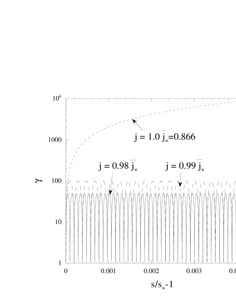
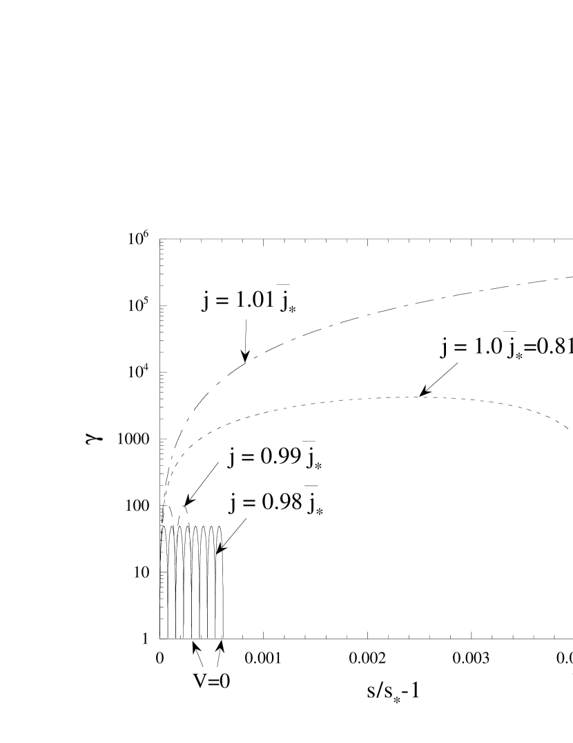
Figure 1: Spatial distribution of $\gamma$ along magnetic field lines. We choose $\theta=0$. (a) represents solutions for the flat spacetime with $r_{g}=\omega=0$. $\gamma$ oscillates or increases monotonically according to $j$. (b) represents GR solutions. In the case of $j<j_{\ast}$ oscillation eventually stops with $V$ approaching zero, in contrast with the non-GR case.

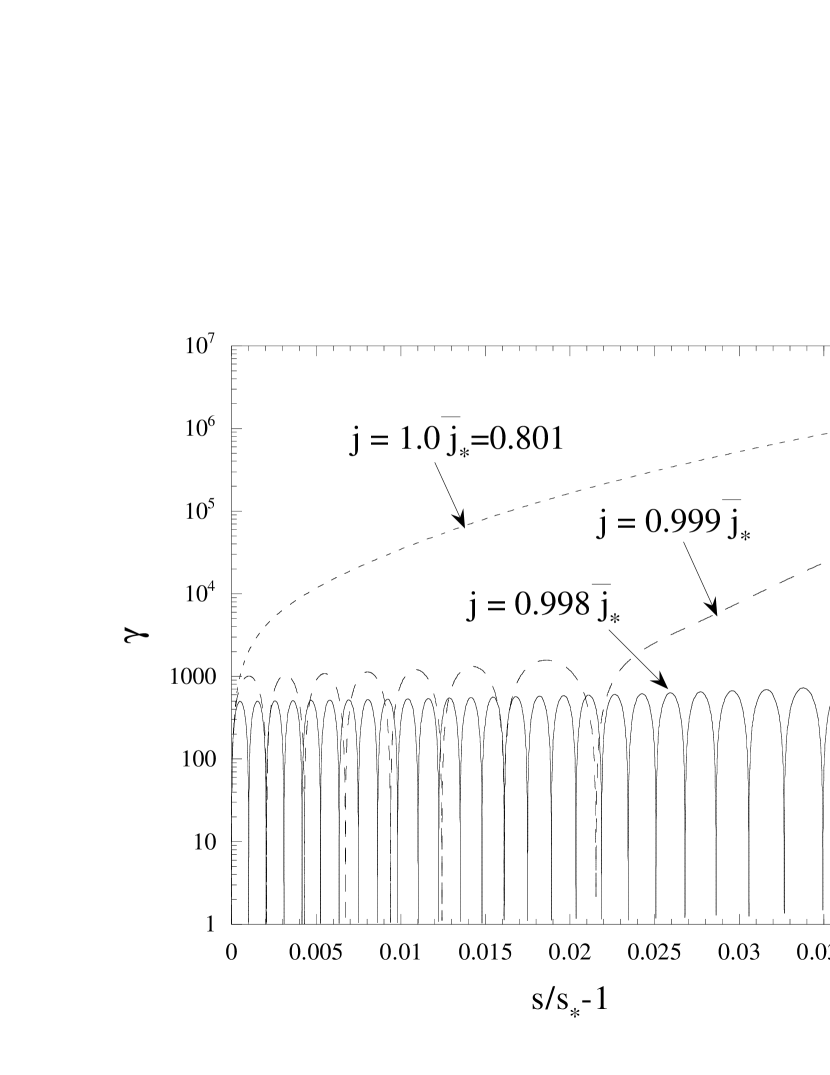
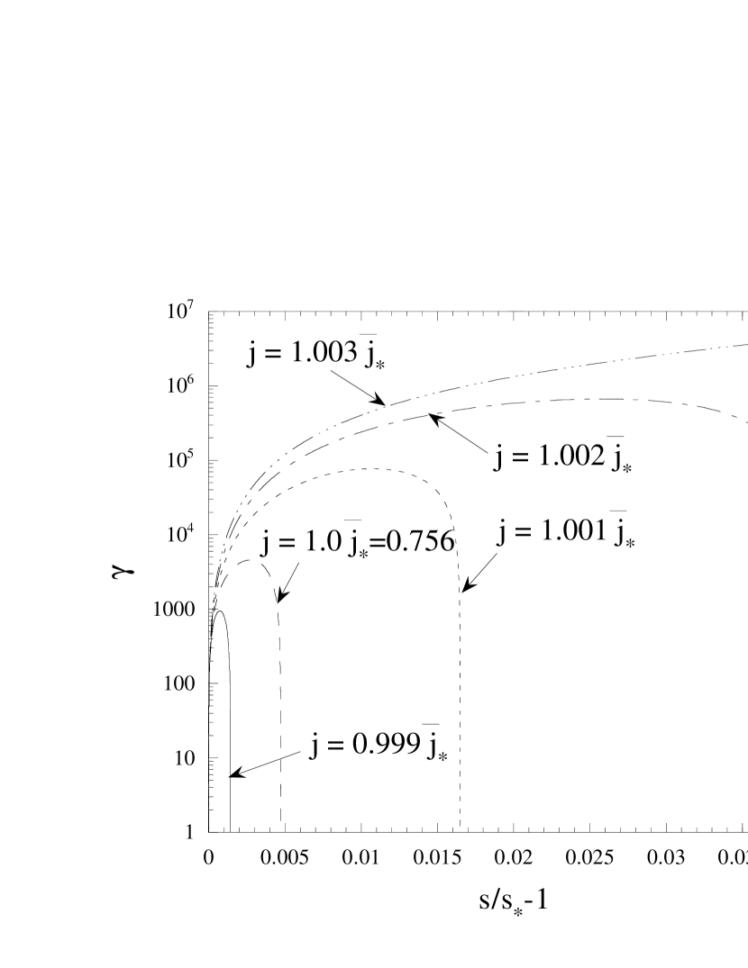
Figure 2: Spatial distribution of $\gamma$ along “away” field lines. We choose $\theta_{\ast}=5^{\circ},~{}\varphi=180^{\circ}$. (a) and (b) represent flat and GR solutions, respectively. Gravity changes particle dynamics for $j<\bar{j}_{\ast}$: acceleration after oscillation does not occur.

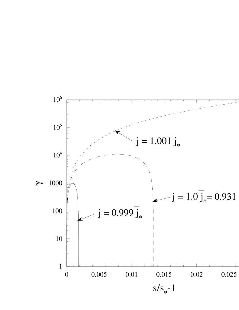
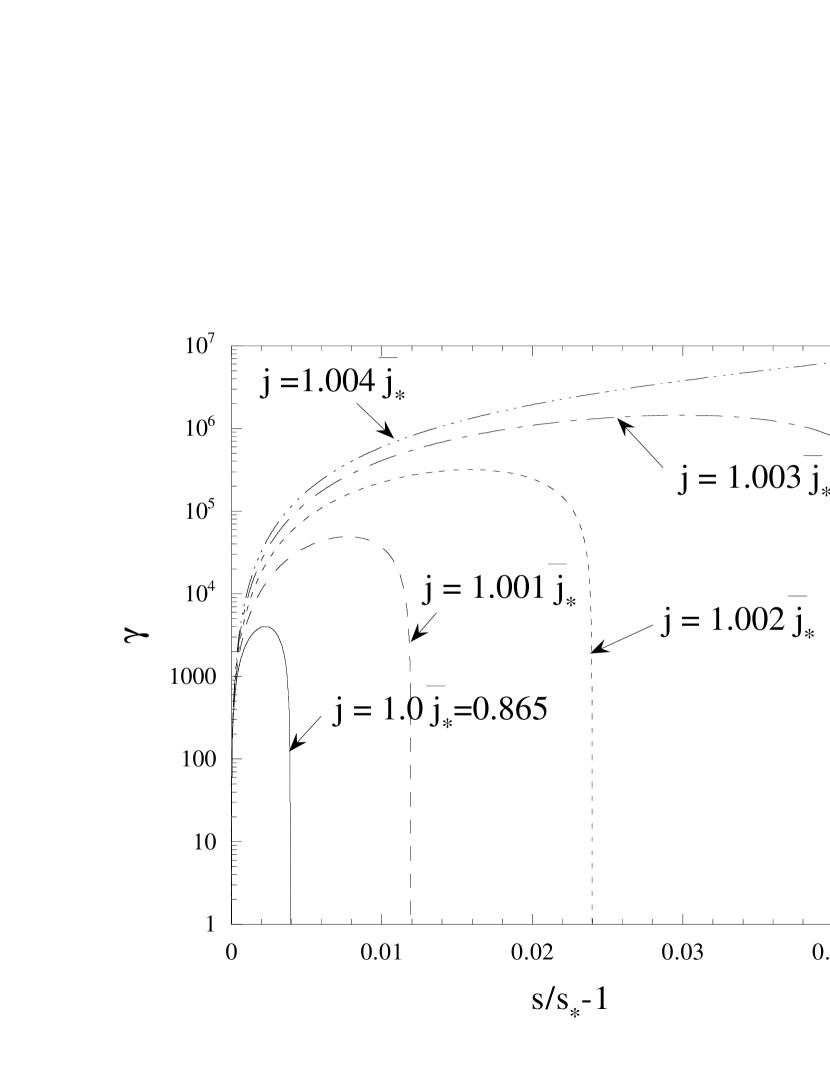
Figure 3: Spatial distribution of $\gamma$ along “toward” field lines. We choose $\theta_{\ast}=5^{\circ},~{}\varphi=0^{\circ}$. (a) and (b) represent flat and GR solutions, respectively.

References

- Arons (1997) Arons, J. 1997, in ”Neutron Stars and Pulsars” eds. Shibazaki, N.,Kawai, N., Shibata, S., & Kifune, T. (Universal Academy Press, Inc.), 339
- Arons & Scharlemann (1979) Arons, J., Scharlemann, E.T. 1979, ApJ, 231, 854
- Ginzburg & Ozenoi (1965) Ginzburg, V.L., & Ozenoi, L.M. 1965, Sov. Phys. JETP, 20, 689
- Goldreich & Julian (1969) Goldreich, P., & Julian, W.H. 1969, ApJ, 157, 869
- Fawley et al. (1977) Fawley, W.M., Arons, J., Scharlemann, E.T. 1977, ApJ, 217, 227 Fawley, W.M., Arons, J., Scharlemann, E.T. 1977, ApJ, 217, 227
- Harding & Muslimov (2001) Harding, A.K., & Muslimov, A.G. 2001, ApJ, 556, 987
- Konno & Kojima (2000) Konno, K., & Kojima, Y. 2000, Prog. Theor. Phys., 104, 1117
- Landau & Lifshitz (1975) Landau, L.D., & Lifshitz, E.M. 1975, “The Classical Theory of Fields” (Pergamon)
- Melrose (2000) Melrose, D.B. 2000, in ASP Conf. Ser. 202, “Pulsar Astronomy: 2000 and beyond”, eds. M. Kramer, N. Wex, & R. Wielebinski, 721
- Mestel (1981) Mestel, L. 1981, in IAU Symposium 95, eds. W. Sieber & R. Wielebinski (Dordrecht, Reidel), 9
- Mestel (1996) Mestel, L. 1996, in ASP Conf. Ser. 105, ”Pulsars: Problems and Progress”, eds. S. Jonston, M.A. Walker, & M. Bailes (San Francisco: ASP), 417
- Muslimov & Tsygan (1992) Muslimov, A.G., & Tsygan, A.I. 1992, MNRAS, 255, 61
- Scharlemann, Arons & Fawley (1978) Scharlemann, E.T., Arons, J., Fawley, W.M. 1978, ApJ, 378, 239
- Shibata (1991) Shibata, S. 1991, ApJ, 276, 537
- Shibata (1995) Shibata, S. 1995, MNRAS, 276, 537
- Shibata (1997) Shibata, S. 1997, MNRAS, 287, 262
- Thorne & Macdonald (1982) Thorne, K.S., & Macdonald, D. 1982, MNRAS, 198, 339
- Weinberg (1972) Weinberg, S. 1972, “Gravitation and Cosmology” (John Wiley & Sons)