HI Narrow Self–Absorption in Dark Clouds
Abstract
We have used the Arecibo telescope to carry out an survey of 31 dark clouds in the Taurus/Perseus region for narrow absorption features in HI ( 21cm) and OH (1667 and 1665 MHz) emission. We detected HI narrow self–absorption (HINSA) in 77 of the clouds that we observed. HINSA and OH emission, observed simultaneously are remarkably well correlated. Spectrally, they have the same nonthermal line width and the same line centroid velocity. Spatially, they both peak at the optically–selected central position of each cloud, and both fall off toward the cloud edges. Sources with clear HINSA feature have also been observed in transitions of CO, 13CO, C18O, and CI. HINSA exhibits better correlation with molecular tracers than with CI.
The line width of the absorption feature, together with analyses of the relevant radiative transfer provide upper limits to the kinetic temperature of the gas producing the HINSA. Some sources must have a temperature close to or lower than 10 K. The correlation of column densities and line widths of HINSA with those characteristics of molecular tracers suggest that a significant fraction of the atomic hydrogen is located in the cold, well–shielded portions of molecular clouds, and is mixed with the molecular gas.
The average number density ratio [HI]/[H2] is . The inferred HI density appears consistent with but is slightly higher than the value expected in steady state equilibrium between formation of HI via cosmic ray destruction of H2 and destruction via formation of H2 on grain surfaces. The distribution and abundance of atomic hydrogen in molecular clouds is a critical test of dark cloud chemistry and structure, including the issues of grain surface reaction rates, PDRs, circulation, and turbulent diffusion.
1 INTRODUCTION
Two relatively distinct phases are generally assumed to exist in the neutral interstellar medium (ISM): atomic and molecular. The atomic phase of the ISM, consisting mainly of hydrogen atoms, is traced by the HI hyperfine transition at 21cm. The molecular phase of the ISM, whose major component – molecular hydrogen – lacks a permanent electric dipole moment and readily excited transitions at temperatures generally encountered, is primarily traced by emission from rarer molecular species such as carbon monoxide. The conversion from atomic to molecular forms occurs on dust grains, where atomic hydrogen sticks and forms H2. This exothermic reaction releases H2 into the gas and keeps molecular clouds molecular. Dissociative processes maintain a population of atoms even inside molecular clouds. Recently, there has been increased interest in atomic species, which prove to be important probes. Two important examples are CI, which is accessible at submillimeter wavelengths (e.g. Phillips, Huggins, Kuiper, & Miller, 1980; Huang et al., 1999; Plume et al., 2000), and OI, which can be observed in the far infrared (e.g. Herrmann et al., 1997; Kraemer, Jackson, & Lane, 1998; Liseau et al., 1999; Lis et al., 2001).
Inside molecular clouds, dissociating UV photons are blocked both by grains and by H2 line absorption (Hollenbach, Werner, & Salpeter, 1971). A significant HI population exists inside molecular clouds maintained by cosmic ray destruction of H2 and additionally as a remnant of the H2 formation process in a chemically young cloud. The atomic hydrogen component inside molecular clouds has fractional abundance ([H]/[H2]) of 0.1 (discussed in Section 6) and is thus the third most abundant gas phase species, after H2 and He. Because the balance of HI and H2 involves grain surface reactions, the density of atomic HI in dark clouds serves as a test of complete chemical networks with reactions both in the gas phase and on grain surfaces. The HI abundance in well–shielded regions can be increased by relatively rapid turbulent diffusion (Willacy, Langer & Allen, 2002), or by general mass circulation (Chièze & Pineau des Forêts, 1989). It is therefore important to establish the presence of HI in the molecular ISM and to determine accurately its abundance.
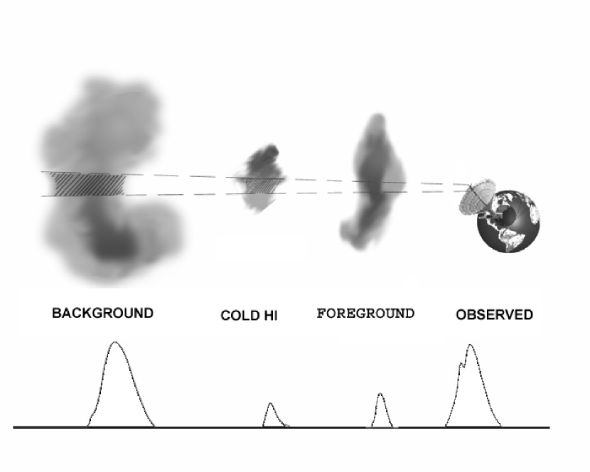
A unique probe of this component is HI narrow (which we define to be less than that of CO) line width self–absorption, which we denote HINSA. The absorption dips seen in the spectra of 21cm emission are often denoted HI self–absorption. The prefix ‘self’ is widely used to differentiate this phenomenon from absorption against a background continuum source. For the origins of HI absorption toward nearby dark clouds, separate galactic background HI emission and cold foreground HI material are both needed. A typical configuration is shown in Figure 1.
The existence of cold HI associated with dark clouds was recognized more than 25 years ago. Knapp (1974) conducted a survey of 88 dark clouds and detected absorption features in fewer than half of them. The optical depth of cold HI was derived from the profiles of the absorption lines. The molecular content of the clouds observed was traced by their dust extinction. The HI fractional abundance, [H]/[H2] was thus determined to be 1% to 5%. In terms of the observational limits and conclusions, this early work typifies most self–absorption studies that have followed.
With the 140ft (43m) telescope, Knapp’s survey has an angular resolution of 21′ and a velocity resolution of 0.5 km s-1. Similar resolutions have been achieved with the 85ft (26m) antenna at Hat Creek (Goodman & Heiles, 1994) and the 120ft (37 m) antenna of the Haystack Observatory (Myers et al. 1978). The 76m Lovell telescope (12′ angular resolution, 0.5 km s-1 velocity resolution; the same convention in what follows) has been employed for a study of six dark clouds in the Lynds (1962) catalogue (McCutcheon, Shuter & Booth 1978) and the Riegel–Crutcher cloud (Montgomery, Bates & Davies 1995). Additional studies have been conducted with the Effelsberg 100m telescope (9′, 0.5 km s-1). The Taurus molecular cloud TMC1 has been mapped by Wilson and Minn (1977). The complex region around B18, also known as Kutner’s cloud, has been mapped by Batrla, Wilson & Rache (1981) and by Pöppel, Rohlfs & Celnik (1983). The Arecibo telescope with the line feed system (3′, 1 km s-1) has been used to study HI absorption (e.g. Burton, Liszt, & Baker, 1978; Baker & Burton, 1979; Bania & Lockman, 1984). Baker & Burton (1979) also raise the possibility that the absorption can help resolve the near–far ambiguity in kinematic distances, a topic which is further explored by Jackson et al. (2002).
Interferometers have also been used to obtain higher angular resolution, but the usual penalty has been lower velocity resolution to augment the sensitivity. Van der Werf et al. mapped L134 (1988) and L1551 (1989) with the DRAO and the VLA (1.5′, 1.3 km s-1). The interferometer studies are well–suited for mapping structures having a scale of arc–minutes. But their velocity resolutions of about 1.5 km s-1 can easily miss or suppress narrow absorption features, which occupy at most a couple of velocity channels in such spectra. To compound this problem, the HI emission is structured. Multiple peaks and wide troughs are not rare in galactic 21c profiles (see, e.g. Figure 2). If a map is based on the integrated area of an absorption line (or lines), the wide troughs which may not be associated with dark clouds will be more prominent than are the narrow features. Reliable analysis of HINSA profile requires a velocity resolution better than 0.3 km s-1.
The general scientific objectives of narrow line HI absorption studies are to explain its origin and to determine the abundance of atomic hydrogen. For the first question, the association of HINSA with dark clouds is inconclusive in the literature. On the positive side, Sherwood & Wilson (1981) find a good correlation with extinction in TMC1. McCutcheon et al. (1978) give a higher detection rate (6–8 out of 11 Lynds clouds) than Knapp (1974). Cappa de Nicolau & Poppel (1991) find HINSA in the ‘darkest’ cores in the CrA complex embedded in a HI emission ridge. On the other hand, the association between HI absorption features and dense regions is ambiguous in a recent DRAO HI survey, in which Gibson et al. (2000) find cloud–like absorption structures both correlated and uncorrelated with CO emission. They label these features HISA, shorthand for HI self–absorption. This is the situation in which the distinction between HISA and HINSA must be made. As seen in the DRAO survey, the HISA probably reflects temperature fluctuations in the atomic ISM. The HISA is spectrally wider and flatter and could have its origin in the same location as the 21cm emitting gas, making its name appropriate. HINSA refers to narrower absorption features, which are produced by cold foreground molecular clouds and which are not prominent in the DRAO survey with 1.3 km s-1 velocity resolution. To further complicate the issue, HI has also been seen in emission in possible halos around molecular clouds, such as B5 (Wannier, Lichten, Andersson, & Morris, 1991). HI halos are a distinct environment for atomic hydrogen compared to either HISA or HINSA, and they are easily distinguished observationally (see Section 7).
The difficulties in obtaining the HI abundance through HINSA are three–fold. First, the early studies are hampered mainly by limited knowledge of the dark cloud itself. The H2 column density is often obtained from low angular resolution extinction data (e.g. Knapp 1974, Batrla et al. 1981) or H2CO (e.g. Wilson & Minn 1977, Poppel et al. 1983), a molecule whose fractional abundance is not very certain. Second, with one profile, it is impossible to obtain both the optical depth and the spin temperature accurately. An assumption about the spin temperature is often made, which may not be realistic. Third, the issue of foreground emission is often ignored.
With some or all of the three uncertainties, the [H]/[H2] ratio has been derived to be ranging from a few percent (e.g. Knapp 1974; Saito, Ohtani & Tomita 1978), to 510-4 (Winnberg, Grasshoff, Goss & Sancisi, 1980).
The requirements of reasonable angular resolution, good sensitivity, and high frequency resolution make the upgraded Arecibo Gregorian system a valuable tool with which to study the HINSA. The large instantaneous bandwidth allows OH 1665 and 1667 MHz spectra to be obtained simultaneously with that of HI. We describe the new observations including a HI survey to examine the correlation between HINSA and OH in dark clouds and complementary mapping in carbon monoxide isotopologues, OH, and CI in Section 2. In Section 3 we present a three–component model for radiative transfer and correction for foreground material, allowing accurate HI column densities to be obtained. We analyze OH and C18O emission in Section 4, and the results of our survey and observations of L1544 in Section 5. We review the general issue of atomic hydrogen in molecular clouds in Section 6, discuss our results in Section 7, and summarize our conclusions in Section 8.
2 Observations
The sources included in our survey of HI in dark cloud cores are mainly chosen from a dark cloud catalogue based solely on optical obscuration (Lee & Myers, 1999). The observed cores meet the following constraints: (1) Right Ascension 2h – 6h, (2) angular diameter close to or larger than 3′, (3) declination angle 0° – 35°, (4) other observing considerations, such as minimizing slew time. Twenty eight cores have thus been chosen for this Arecibo survey of dark clouds Their names, coordinates, presence of HINSA, and association with a young stellar object are given in Table 1. In addition, two well studied dark clouds in Perseus, Barnard 1 (B1) and Barnard 5 (B5), are included in our survey. B1 is one of the few dark clouds with a positive Zeeman detection (Goodman et al., 1989). The physical conditions of B5 have been well determined through mapping of CO and its isotopologues (Young et al., 1982). The inclusion of these two sources also extends the length of the nightly observing session at Arecibo, due to their early rise times. Because there is no a priori knowledge regarding the HINSA properties of B1 and B5, they should not bias our study of the correlation between HINSA and dark clouds. TMC1 is a well studied region with both strong OH emission and HI absorption. We observe TMC1CP, the cyanopolyyne peak of TMC1 (Pratap et al., 1997), as a secondary calibrator source to check the consistency of data taken at different times. Because it is a previously known strong HINSA source (Wilson & Minn 1977), TMC1CP is excluded from source statistics presented later. In summary, our sample has 30 sources plus TMC1CP as a calibrator.
L–band observations of nearby dark clouds were conducted at Arecibo in September 1999, February 2001 and January 2002. The 3′ beam size corresponds to about 0.13 pc at the 140 pc distance of the Taurus dark cloud complex. Most individual nearby clouds fill the main beam at this frequency. The Arecibo spectral line correlator is configured to observe HI and OH (1665 MHz and 1667 MHz) simultaneously. The two lines of OH and the 21cm line of HI are recorded with a channel width of 0.382 kHz, which after smoothing yields a velocity resolution of 0.14 km s-1 for OH and 0.16 km s-1 for HI. The remaining section of the correlator is employed to record the HI profile at a lower resolution with a wider bandwidth. This is necessary for obtaining a good spectral baseline when the HI emission toward some sources is nearly as wide as the bandpass at the higher resolution, as does occur for some sources (e.g. L1578–2).
The data were taken in a total power (ON scan only) observing mode. The prevalence of background HI emission and its variation on an arc–minute scale make finding clean OFF positions very questionable. Especially in regions of extended emission, such as the Taurus dark cloud complex, the use of an OFF position can lead to large uncertainties caused by variation in the emission. Sources such as CB 37, shown in Figure 2, illustrate such fluctuations across the band with amplitude comparable to the narrow absorption feature. In a study of HI envelopes, Wannier et al. (1983) find in their sample that the average variation of HI emission across a cloud boundary is 10.9 K at the molecular emission velocity. Fortunately, the narrowness of the absorption dip of interest, together with the stability of the Arecibo system, makes possible the measurement of the line profile even without an OFF scan (see Section 3). In addition to the reduction in the uncertainty due to emission in the OFF scan, the stability of the system also allows a factor of 2 reduction in the statistical fluctuations by eliminating any switching.
The correction for the elevation dependence of the antenna gain and the absolute calibration are carried out by observations of quasars. By cross–scanning these strong point sources, beam maps are also obtained to measure the size of the main beam. In all the data reduction which follows, we treat the slightly elliptical beam to be a circular one with the same solid angle. The derived aperture efficiency is 64% and the main beam efficiency 60%. All L–band data are corrected for the main beam efficiency. This is exact if the source just fills the main beam, and appears to be close to an optimum strategy for a one–parameter calculation.
Each ON source position was observed for an integration time of 5 to 10 minutes. At the current sensitivity of Arecibo ( K), Galactic HI profiles without ambiguity caused by noise can be obtained in an even shorter time. The RMS noise level of less than 0.1 K in all our spectra is set by requirement of detecting OH lines, which typically have antenna temperatures in the range of 0.5 K to 1 K. The beam efficiency for data taken in Feb 2001 is significantly higher than it was previously, as a result of surface readjustment for the primary. Relative calibration and consistency checks are carried out using the strongest source, TMC1CP, which was observed both before and after the surface readjustment. The data from 2001 observations were scaled to those obtained at the earlier epoch, when extensive quasar calibration observations were made.
To determine the H2 column density reliably, C18O data on cores with clear HINSA were obtained in October 2000 at the Five College Radio Observatory (FCRAO). The ‘footprint’ size of the 16 element SEQUOIA focal plane array is 5.9′5.9′. We use four pointings to make a beam sampled map of each source and convolve it with the Arecibo beam. The data are corrected for the main beam efficiency to give the best estimate of the total mass in the beam as discussed above. By combining C18O and HI data, the abundance [H]/[H2] can be obtained. At FCRAO, CO and 13CO spectra were also obtained for comparison with HI absorption line profiles.
The 492 GHz ground state fine–structure line of atomic carbon (CI) has also been observed by the Submillimeter Wave Astronomy Satellite (SWAS) toward clouds with clear HINSA features. In PDR models, CI should be abundant only in low extinction regions. We compare its line characteristics to those of HINSA to examine the importance of photodissociation in maintaining populations of low temperature HI.
3 Three–component Radiative Transfer and Foreground Correction
3.1 Radiative Transfer
The standard approach for analyzing absorption is to reconstruct the emission spectrum from observing one or multiple ‘OFF’ positions, where the absorption is absent. As noted in section 2, identifying such OFF positions is problematic for HINSA. However, the emission spectrum can still be estimated for HINSA because the absorption line is much narrower (typically a factor of 20) than the background emission. The instrumental baseline is both flat and stable, which allow us to use only the ON spectra.
The reconstruction is carried out by fitting a 5th–order polynomial across the frequencies affected by the absorption in the HINSA spectrum to define the profile as if there were no absorption present. The details and uncertainty associated with such a fit will be discussed in the following subsection.
The classical problem of deriving two quantities, the optical depth and the excitation temperature from one profile is compounded by the possible foreground contamination, which adds more unknowns to the mix. A careful look at the radiative transfer is necessary before any quantitative analysis of the HINSA can be carried out with confidence.
A three–component model is outlined in Figure 1. It represents a general view of the HI absorption in the galaxy. The parameters are defined as
-
•
: background HI temperature ,
-
•
: foreground HI temperature,
-
•
: background HI optical depth ,
-
•
: foreground HI optical depth,
-
•
: excitation temperature of HI in the dark cloud ,
-
•
: optical depth of HI in the dark cloud,
-
•
: continuum temperature, including the cosmic background and Galactic continuum emission.
The antenna temperature produced by the three–component system is
| (1) |
To focus on the effect of the intervening dark cloud, the Galactic atomic gas is assumed to be of uniform temperature () and small optical depth () at 21 cm. We can then write
| (2) |
and
| (3) |
To consolidate the variables, we define
| (4) |
For our ON spectra, a linear baseline is removed along with the passband shape. Since the background continuum is flat across the band in our observations, it is also removed through our baseline fitting procedure. Thus, the effective spectrum is given by
| (5) |
Another quantity is obtained from the spectrum by fitting a polynomial to the portion of the spectrum without the absorption. We call this quantity ,
| (6) |
which is the HI temperature that would be observed if there were no absorbing cold cloud and under the assumption outlined in equations (2) and (3).
Taking the difference of and , we can obtain, as a positive quantity, the absorption temperature
| (7) | |||||
For small foreground and background HI opacities and with the definitions of and , the absorption temperature can be written as
| (8) |
where and are observables and is the quantity desired from the analysis. The explicit dependence on the HI emission temperature is eliminated. Let us examine the remaining unknowns, , , , and .
The fraction of the HI along the line of sight lying beyond the cloud responsible for the absorption, , can be calculated from a model of the local HI distribution. To first order, the Galactic HI disk can be approximated by a single Gaussian with a full width half maximum (FWHM) vertical extent equal to 360 pc (Lockman, 1984). The percentage of HI in the background is thus given by the complementary error function
| (9) |
where D is the distance to the absorbing cloud, b is its galactic latitude, and .
The Galactic background emission is estimated to be about 0.8 K by extrapolating the standard interstellar radiation field (ISRF) to L–band (e.g. Winnberg, Grasshoff, Goss & Sancisi, 1980). = 3.5 K is thus used in the analysis which follows.
The excitation temperature of the 21cm line in dark clouds, , is determined by the balance between collisional and radiative processes. Ignoring radiative trapping, the solution to the two level problem is given by Purcell & Field (1956) as
| (10) |
where , the excitation temperature of the 21cm line in our terminology, is also called the spin temperature, is the kinetic temperature of the gas in the dark cloud, and is the effective temperature of the radiation field given above. The quantity y is defined by
| (11) |
where is the collisional deexcitation rate and is the spontaneous decay rate, s-1 (Wild, 1952). There have been various calculations of the collision rates for the deexcitation of the 21cm line, but the most relevant are the spin–exchange collisions with another hydrogen atom (Field, 1958; Allison & Dalgarno, 1969). The collisional deexcitation rates calculated with a full quantum scattering code in the latter reference are considerably smaller than values determined earlier, and for a temperature = 10 K yield a value y = 5.5, where is the atomic hydrogen density in cm-3.
For y 1, the excitation temperature approaches the kinetic temperature of the gas. This requires an atomic hydrogen density of at least 1 cm-3. As we show in the following, this is a reasonable value for the atomic hydrogen density. Inside dark clouds, most of the hydrogen is in the form of molecules. But as discussed in Section 6, a steady state HI density is maintained by cosmic ray destruction of H2; this density is independent of the density of H2. The standard model gives cm-3, in reasonable agreement with our observations. Thus, the assumption of thermalization is justified. For lower densities, since is less than , the excitation temperature will be below the kinetic temperature.
The effect of the foreground comes in two terms in equation (8), and the change in due to the foreground absorption is equal to . The excitation temperature is close to the kinetic temperature of dark clouds, which is always lower than the HI emission temperature . Since p is generally in the range 0.8 to 0.9 and since is only a few tenths, is the dominant term for our HINSA observations. This means that becomes smaller due to the existence of foreground HI gas. The uncertainty in the derived HINSA column density resulting from our not knowing the exact value of will be discussed in the following subsection.
Finally, the peak optical depth of the absorption feature at the centroid velocity can be obtained using equation (8)
| (12) |
which in turn gives column density of HINSA as
| (13) |
where is the FWHM of the absorption line from a Gaussian fit.
In summary, the recipe we have used for obtaining the HINSA column density involves, first, fitting the emission line profile to determine THI, second, using a model of the Galactic HI to determine p, and third, deriving the peak optical depth of the cold HI through equation (12). Fourth, we use equation (13) with the line width fitted to the absorption feature, to determine the column density. By fitting the emission and absorption portions of the spectra separately and using these two fits, the optical depth of the absorption alone can be derived without explicitly knowing the background and foreground temperatures, as long as they are equal and the galactic HI emission is optically thin.
3.2 Uncertainties
The OH intensities are 10 to 200 times smaller than of HI emission. At the current level of integration, which is chosen to ensure good OH detections, the noise in HI spectra is insignificant. The uncertainties in the derived HINSA column density result primarily from three aspects of the assumptions behind and modeling of the radiative transfer.
First, the imperfect knowledge of the Galactic HI disk and the cloud distance results in uncertainties in . For 5 clouds, the distance is not known and cannot be modeled. The remaining clouds have an average . The difference between unity and this average provides us an idea of the uncertainty in . According to equation (12), this results in a 30 uncertainty for the derived optical depth and, in turn, the column density.
Second, the fitting to the background is somewhat arbitrary. The upper panel of figure 3 demonstrates the effect of using different orders of polynomial. The maximum difference in the fitted temperatures is 1.1 K and that in linewidth is 0.14 km s-1. Higher orders of polynomial usually do not work well. A Gaussian fit to the background is not feasible for sources with very structured HI emission profiles, such as L1574 and L1633. The magnitude of the uncertainties also depends on the position of absorption relative to the peak emission. When absorption occurs closer to the emission center than the situation shown in Figure 3, the uncertainty in the antenna temperature becomes larger and the uncertainty in the linewidth becomes smaller. We take 2 K as a representative value of uncertainty in the temperature and 0.15 km s-1 as that for the line width. These values are also included in Tables 2 and 3. In the lower panel of figure 3 shows the change in the peak HINSA optical depth produced by the uncertainty in the fitting of the background HI emission. A deviation of 2 K in temperatures (both and ) results in a change in by 0.04. This is 14 relative to the average optical depth of the absorption.
Third, we consider the uncertainties in the term. In order to conform to the general assumptions of an optically thin HI emission (), the value of is thus between 0 and about 0.1. With K, 3.5 K and typical numbers for , this corresponds to a change in of absorption of about 0.01, which is 4 relative to the average optical depth. We conclude that the uncertainty in the derived HINSA column density is dominated by systematic effects, and the overall uncertainty is approximately 50.
4 Analysis Techniques for Spectral Lines with Small Opacities
4.1 OH Column Density
From the definition of opacity, the column density of OH can be written as
| (14) |
where s-1 is the A coefficient of this transition and is its excitation temperature. Under the assumptions of negligible optical depth and no background emission, the column density can be calculated from the integrated intensity (in K km s-1) of the 1667 MHz line through (e.g. Knapp & Kerr, 1973; Turner & Heiles, 1971)
| (15) |
The satellite component of this doubling line at 1665 MHz can be useful in determining the the optical depth and excitation temperature. For emission without anomalies, the antenna temperatures of the two components satisfy
| (16) |
where . The ratios for our sources range from 1.2 to 1.9, with the majority being around 1.8. This confirms that we are seeing thermal emission from dark clouds and that the opacity is only modest. Equation (16) gives a unique solution for , which leads to
| (17) |
Except for one source, the excitation temperature of OH ranges from 5 K to 9 K, which is not much larger than the background temperature. At this level of excitation, the assumption of neglible background temperature made for equation (15) results in underestimation of by a factor of 1.6 to 2.3.
Because of weaker line emission at 1665 MHz and the exponential dependence of the antenna temperatures on the optical depth, the satellite line ratio method is very sensitive to uncertainties in the spectra of the satellite component. In some cases, the line widths of the main and the satellite line are not the same, which may be a result of the low signal to noise ratio of the satellite component. To present a more self–consistent correlation study of HI and OH, we only use the 1667 MHz data in determining OH column density, but note that these results likely underestimate the OH column density by a factor 2.
4.2 C18O Column Density
In order to determine the molecular content of dark clouds, we have chosen as a tracer the J=1–0 transition of C18O, which is optically thin (or close to it), and which has relatively uniform abundance relative to H2, (Frerking, Langer & Wilson, 1982). The C18O column density in the J=1 level can be calculated from
| (18) |
where is the excitation temperature of the J=1–0 transition, is the background temperature, and the integrated intensity is corrected for the main beam efficiency. The LTE approximation is then used to justify substituting for for all transitions in converting to the total column density of C18O. The smoothing of the FCRAO (45″ beam) data to the Arecibo resolution gives a physical meaning to the [H]/[H2] thus derived: it is the ratio between the total number of H atoms and H2 molecules in a 3′ beam.
5 HI Survey Statistics and Characteristics of HINSA
As described in Section 2, we surveyed 30 nearby dark clouds, unbiased in terms of HI absorption. In this sample, 23 have a clear narrow absorption dip at the same velocity as that of the OH emission (Figures 4 & 5). Four more clouds (L1498, L1506B L1622A & L1621-1) have hints of an absorption feature coincident in velocity with the OH emission, which correspond to a ‘shoulder’ on the HI profile (Figure 6). The remaining three clouds (B1, B5 & B213-7) have no indication of narrow absorption features. Counting the clouds with the ‘shoulder’ features as non–detections, the detection rate of HINSA toward optically selected dark clouds is 77 percent. This high detection rate strongly supports the association of HINSA with dark clouds. Further analysis given below based on comparisons of specific tracers reinforces this association.
In our sample of 30 dark clouds, 7 are found to contain embedded young stellar objets (EYSO) (Lee & Myers, 1999). The ratio of cores with EYSO to starless cores is thus 0.3, the same as found in these authors’ larger sample. If the detection rate of HINSA is independent of EYSO, we would expect to find 17.6 clouds with HINSA in starless cores and 5.4 clouds with HINSA in EYSO cores. The actual numbers in our sample are 17 and 6, respectively. Thus, our observations indicate that the presence of an embedded YSO does not significantly affect the likelihood of finding HINSA.
In our sample, the HI spectra are often structured and some are most likely due to multiple absorption features (e.g. L1517C, L1512, L1523, CB37, CB45 and L1633). Out of these multiple absorption features, only those with corresponding molecular emission are believed to be associated with molecular clouds. In our sample, these features exhibit a line width comparable to that of 13CO at the same velocity. We therefore define HI self-absorption features with corresponding CO emission and line width smaller that of CO as HI Narrow Self–Absorption (HINSA). This view is compatible with the findings of cold HISA features without molecular counterpart in the Canadian Galactic Plane Survey (Gibson, Taylor, Higgs, & Dewdney, 2000; Knee & Brunt, 2001). The Arecibo HI survey of the galactic ring (Kuchar & Bania, 1994) also shows extended HI absorption feature without overlaying CO clouds. The existence of atomic hydrogen colder (15 K to 35 K) than the standard value (80 K) for the Cold Neutral Medium (CNM), yet still independent of molecular clouds, has also been indicated in studies of absorption against continuum sources (e.g. Heiles, 2001). Most of the HISA is thus likely a result of temperature fluctuations in the CNM. In the absence of molecular cooling, it is still not evident how atomic gas can be maintain at such low temperatures. In contrast, the low temperatures of HINSA have a straightforward explanation in terms of CO cooling if it arises in largely molecular regions. Clouds with HINSA are also less turbulent than typical “neutral hydrogen” clouds that may produce HISA, further emphasizing the distinction between the two.
5.1 Low Temperature of the HINSA
There are two ways to estimate the temperature of the atomic hydrogen detected in absorption.
First, the line width of the absorption dip provides an upper limit to the kinetic temperature assuming only thermal broadening is present. The equivalent temperature, derived from the fitted FWHM () of HI absorption
| (19) |
is given in Column 13 of Table 2. There are 10 sources which have an absorption line width so narrow that the HI responsible must be thermalized, or be very close to thermalization, at a temperature lower than 15 K. The narrow line widths we have observed rule out the possibility that the HINSA could be produced in warm (e.g. cloud halo) gas with T 100 K, even allowing for modestly subthermal excitation of the 21cm transition.
Subtle complications in obtaining line parameters from an absorption feature arise when the dip is on the slope of the background emission. In general, the fitted absorption line appears to peak closer to the center of the emission feature, and to appear narrower than it really is. The corrections required in both cases are small compared to the line width of the narrow line HI absorption. We do not correct for the displacement of velocity peak, since the average effect is zero due to the randomness of the dark cloud velocity with respect to that of the background HI emission. The correction for line width is on the order of 0.04 km s-1 (Levinson & Brown, 1980), which is only significant when calculating for a couple of unusually narrow line width sources. The uncertainty thus introduced in for L1523, L1521E and L1517B is between 0.5 K 1 K. For other sources, this correction can be neglected.
Second, the excitation temperature (or the spin temperature for the 21cm line) can be estimated by rewriting equation (8)
| (20) |
The optical depth of the narrow line absorbing gas is on the order of unity. Substituting an infinite into the equation above overestimates . For the optical depth of the foreground emission , a nominal value of 0.1 is used, which is probably an overestimate obtained by assuming the total optical depth of galactic HI emission () to be unity. The upper limit of HINSA excitation temperature is thus
| (21) |
These upper limits are listed in Column 14 of Table 2. Compared to the temperature limit set by the line width, this method has relatively large uncertainties resulting from the assumptions about and the optical depth. Nonetheless, it provides an independent estimate based on the depth of the HINSA profile. It also confirms our understanding that the majority of HINSA features come from cold gas ( K) with some sources in the range of 10 K.
These two estimates of temperature upper limits reveal HINSA to be associated with cold gas. According to the lower value between the two upper limits, the average temperature upper limit to the 24 HINSA features is 23 K. Moreover, a significant fraction of the sources must have atomic gas as cold as 7–15 K. The well shielded regions of molecular cloud cores are the most likely, if not the only, sites that can plausibly contain material this cold.
5.2 HI and OH Correlation
For sources with well defined absorption features, the similarities between the OH and HINSA profiles are obvious. The two profiles are coincident in velocity as shown in Figure 7.
The line widths of different species are important indicators of the conditions in the regions they are found, as well as of the extent of the regions responsible for the spectral line in question. The well known empirical velocity–line width relations all suggest larger line widths at larger spatial scales (e.g. Larson 1981; Caselli & Myers 1995). To compare the line widths of species with very different molecular/atomic weight, it is appropriate to separate the thermal from the nonthermal contributions to the line widths. This can be done by defining the nonthermal line width as
| (22) |
where is the observed FWHM of the line, is the molecular or atomic weight, is the hydrogen mass and is Boltzmann’s constant. For HINSA, the width is that of the Gaussian fitted to the absorption profile, while for the other species we fit the emission spectra. The correction for the thermal broadening is significant for the HI due to its low mass. The nonthermal line width gives a better indicator of the spatial extent of its progenitor, since the mass dependence of the thermal broadening has been corrected for. The line width data can be found in Table 2.
It is evident that the HINSA, OH, and C18O line widths are well correlated, while the CI exhibits quite different behavior. The average nonthermal line width of the HINSA and of the OH are 0.85 km s-1and 0.83 km s-1, respectively. They are essentially the same as the average line width of 13CO at 0.82 km s-1. These results indicate that the HINSA is produced in regions of significant extinction where the molecular abundances are appreciable.
We have obtained direct information on the spatial correlation of HINSA and OH emission by extensive mapping of L1544, discussed below in Section 5.4. Limited evidence for spatial correlation of OH and HINSA can also be found by looking at the OFF source spectra (Figure 2). When the telescope beam is moved away from the center of each source, it is evident that the HINSA absorption dip starts to disappear along with the OH emission. There is no hint of any increase in the strength of the absorption features at the cloud boundaries, as would be expected if the gas producing the HINSA were in some peripheral zone of the clouds we have studied 111We hesitate to use the term ‘limb brightening’ to describe an increase in the depth of the absorption line, but if the HI in question were in an outer ‘onion skin’ of the cloud, a map of the integrated area of the absorption would presumably exhibit this behavior..
5.3 Correlation with CO Isotopologues and CI
As listed in Table 2, all observed species, HINSA, OH, C18O, and CI, have essentially the same velocity relative to the local standard of rest () in a given cloud. The Vlsr of the HINSA and of the C18O are plotted in Figure 7. The root mean square separation of our data points from the line of equal velocities is 0.03 km s-1, which is small compared to both the line width and the velocity resolution.
As traced by the line widths, the spatial distributions within the clouds of the CO isopologues, the HINSA, and the HI appear to be somewhat different. As mentioned above, HI, OH, and 13CO have, on average, the same line width. C18O has the narrowest line width ( 0.64 km s-1), presumably tracing the innermost core. The CO line is wider with = km s-1, while the CI line is much wider still with = 2.3 km s-1. The large nonthermal line width of the CI confirms this species to be a tracer of PDR regions, where more turbulence exists. HINSA seems to be mixed with relatively quiescent molecular material at higher extinction.
For individual sources, a positive correlation exists between the line width of OH and of HINSA, as shown in the upper left panel of Figure 8. The probability of the null hypothesis (the two being uncorrelated) is = 3.6; the linear correlation coefficient is 0.76. A similar correlation exists between the OH line width and that of C18O. In contrast, no such correlation exist between the OH and CI line widths. Again assuming a linear correlation, the null hypothesis is very likely ().
For the column densities, only OH and C18O are definitely positively correlated. For HINSA, the correlation is not clear. This is somewhat expected from the standard H2 formation model (section 6), as the column density of HINSA should be correlated rather with the cloud size than with that of H2. For CI, the assumption of small optical depth has not been tested in our study and thus may cause large uncertainties. The current data set does not definitively answer all questions about the correlation between column densities of the different species, a subject which deserves additional consideration.
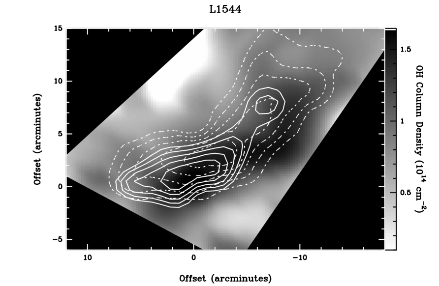
5.4 L1544
To get a better idea of the spatial correlation of HINSA and molecular tracers, we mapped the quiescent dark cloud L1544. This object has relatively narrow line widths in molecular tracers ( km s-1; km s-1). It is usually characterized as starless, due to there being no clear association with an IR source (Ward-Thompson, Scott, Hills, & André, 1994). The inner 5′ core region around the center of L1544 has been well studied and found to exhibit molecular depletion and infall motions (Caselli, Walmsley, Zucconi, et al., 2002; Tafalla et al., 1998).
We mapped an extended region of L1544, which is the same area as outlined by extinction (Snell, 1981). The RMS of our HI and OH spectra are smaller than 0.1 K. At the cloud periphery, the OH 1667 MHz emission is generally weaker than 3 . All three tracers, OH, HINSA, and C18O delineate the same cloud (Figure 9). The H2 column density in the center of this cloud derived from C18O and assumed standard fractional abundance is 6.5 cm-2. Taking dimensions of the cloud core of 9′ by 16′ gives a characteristic size of 0.49 pc at an assumed distance of 140 pc. This results in a characteristic volume density (H2) = 4.3 cm-3.
For a spherical cloud of uniform density in virial equilibrium ignoring magnetic fields and external pressure, the H2 density is given by
| (23) |
where is the FWHM line width, is the cloud radius, and is the mean molecular weight. Substituting the appropriate values yields cm-3. This is in reasonable agreement with the average density derived above, and suggests that this cloud is in, or not far, from virial equilibrium.
The secondary maximum in OH located around offsets (-8′, 3′) is due to a localized increase in the line width, indicating an increase in turbulence. At the center of the cloud, the line width of the 1667 MHz OH emission is 0.47 km s-1, while at (-8′, 3′), it is 0.70 km s-1. This second, more turbulent peak in the OH column density does not correspond to an enhancement in either C18O or HINSA. A likely scenario is that the OH traces a low extinction envelope, which exhibits fluctuations in MHD or some other kind of turbulence, while C18O represents the total column density of quiescent material. HINSA produced by cosmic ray dissociation (see Section 6 below), which is unaffected by extinction, should also be able to trace the highest column density regions. On the other hand, if HINSA is produced mainly by photodissociation in the envelope, a limb brightening effect should appear. Such an effect is not seen for L1544.
A recent study has also indicated a correlation between HI self–absorption and molecular emission for the molecular cloud GRSMC 45.6+0.3 (Jackson et al., 2002). That study, however, suggests that HI absorption arises from cloud skins with . Even at its near distance of 1.8 kpc, this source is more than an oder of magnitude more distant that of L1544, so the detailed location of the cold HI relative to the molecular material is hard to be determined with confidence. Our study of L1544 favors a “distributed” rather than an “external skin” layer for HI, but this conclusion should be confirmed by additional detailed maps of nearby clouds.
6 The Atomic Hydrogen Density in Molecular Clouds
The majority of molecular hydrogen in the ISM is thought to be formed by reactions on dust grains. This process is also the major destruction pathway for hydrogen atoms. The steady state H2 production rate (cm-3 s-1) can be written as
| (24) |
where is the grain number density, is the HI density in the gas phase, is the grain cross section, is the relative velocity between H atom and grains (essentially the velocity of H), is the sticking probability of an H atom on a grain, and is the formation efficiency. The total density of hydrogen atoms is = , where is the density of hydrogen molecules. The grain and proton number densities are related through . The value of depends on the grain model and gas conditions. A ‘standard’ dust grain is taken to have a radius of 0.1 m and a density of 3 g cm-3. In a molecular cloud, we can reasonably assume the following gas conditions: [He]/[H] equal to 0.09, most hydrogen gas in the form of H2, and an gas to dust mass ratio of 100. Based on these assumptions about the dust grains and the gas, we determine to be .
In the standard picture of H2 formation (Hollenbach & Salpeter 1970), the time scale for H atoms deposited on the grain to ‘cover’ the grain surface through tunneling processes is much shorter than the residence time of an adsorbed H atom. Since the H2 formation reaction is exothermic (4.5 ev released), is taken to be 1 in their model as long as there are more than two H atoms on a grain. Equation 24 with a near unity works well in diffuse clouds with S0.3 (Hollenbach & Salpeter, 1971; Jura, 1975). A recent study of sticking probability on icy surfaces gives close to unity at low temperatures (Buch & Zhang, 1991). A recent analysis including both chemisorption and physisorption on grain surfaces indicates that H2 formation can be efficient over a wide range of temperatures (Cazaux & Tielens, 2002), specifically including the 8 K - 20 K range of interest for dark clouds. Adopting and = 1.0 for the following discussion, we obtain the equation
| (25) |
where is the gas temperature, for the formation of rate of H2.
For typical dark cloud conditions with temperature of 10 K, cm-3, the HI to H2 conversion time scale, /R, is approximately 0.5 million years. Such a rapid conversion leaves an essentially ‘molecular’ cloud in which the atomic component is maintained by cosmic rays in a steady state. The destruction rate of H2 is n2 (cm-3 s-1), where s-1 is the cosmic ray ionization rate. This parameter has approximately a factor of 3 uncertainty associated with it, as indicated by the varied results and range of fits obtained for different sources and models by e.g. Caselli, Walmsley, Terzieva & Herbst (1998); Caselli, Walmsley, Zucconi, et al. (2002). In a steady state and assuming n2 n1,
| (26) |
which, for 10 K, gives n1 to be 2.3 cm-3.
This HI density is independent of the local gas density 222 This is by no means a new result; e.g. Solomon & Werner (1971) showed that a constant was to be expected, although their value was more than an order of magnitude larger due to the large value of the cosmic ray ionization rate which they adopted.. Therefore the entire region containing molecular material can contain cold HI and be capable of producing HINSA, with essentially an equal contribution per cm of path along the line of sight. In our sample of clouds, the average column density of HINSA is 7.2 cm-2. We adopt an angular size for the region with absorbing HI of 15′, which is consistent with the typical size of Lynds clouds and Bok globules in the Taurus complex. This corresponds to a physical dimension equal to 0.6 pc at a distance of 140 pc. The average H2 gas density which we derive from the average column density of C18O and fractional abundance 1.7 is equal to 2.5 cm-3. The average HI fractional abundance [HI]/[H2] in the dense molecular gas predicted from the standard theory is 9.2. This is in reasonable agreement with the observed result 1.5 (see Table 3 and Figure 10).
Another obvious process for producing atomic hydrogen associated with molecular clouds is photodissociation. In a plane parallel PDR model with microturbulence (Wolfire, Hollenbach, & Tielens, 1993; Jackson et al., 2002), a large fractional abundance of HI () can be produced at low extinctions (). We do not see this HI envelope, either in total column density or in morphology. One possible explanation is that the conditions in such regions are much less favorable for production of HINSA than the cold, quiescent regions of the clouds. If we ignore foreground and background absorption as well as any continuum, we see from equations (8) that the magnitude of the absorption line from the optically thin, thermalized gas responsible for the HINSA in the cloud is
| (27) |
where is the excitation temperature of the atomic hydrogen. As the temperature in the PDR region rises, so does , and the absorption intensity drops; as approaches the background temperature, the drop becomes precipitous. In these externally ionized and heated regions, it is reasonable that the turbulence, and hence the line width, is considerably greater than in the quiescent cloud material, which also weakens the absorption per hydrogen atom.
As pointed out by Wolfire, Hollenbach, & Tielens (1993), the microturbulent model has difficulty in reproducing CO 1–0 line profiles. Another scenario is clumpy cloud models with macroturbulence. The difficulty with such models is that the observed line profiles are usually very smooth, which is hard to reproduce by a clumpy structure. It would be very interesting to see the predictions of PDR models and radiative transfer calculations with numerous tiny clumps.
7 Discussion
Through observations of HINSA, we have identified cold atomic hydrogen associated with molecular clouds. A detailed explanation of HINSA and related molecular species would require comprehensive models, which may involve PDR, clumpy structure, gas and grain surface chemistry (Ruffle & Herbst, 2000), and possibly other effects such as turbulent diffusion (Willacy, Langer & Allen, 2002). An accurate determination of the abundance of cold HI and its spatial distribution thus constitutes a severe test of the chemistry and physics of ‘molecular’ clouds.
A steady state calculation using standard cosmic ray rate and H2 formation rate is shown to produce approximately the amount of cold HI observed. The data do suggest, however, that there may be a need for modest additional sources of atomic hydrogen in cold molecular regions.
The simple steady state model may not be an accurate or complete picture, however; with improved confidence in the H2 formation rate, the HI fractional abundance we have observed can be used to put an upper age limit on these clouds. The question of whether the H2 formation rate does slow down in dense cores can be answered by observations at higher spatial resolution (′), which will either identify HINSA features correlated with high density tracers, or show HINSA to be smooth on such scales.
HINSA traces different population of neutral hydrogen from that constituting the warm HI halos also associated with molecular clouds (Andersson, Wannier, & Morris, 1991). The HI halos are mostly seen by virtue of the enhancement of HI emission around molecular clouds. Statistically, the HI emission maxima have been shown to lie outside the clouds as defined by their CO emission (Wannier, Lichten, Andersson, & Morris, 1991). Such halos have to be warm to be seen in HI emission with the galactic background. In fact, the absorption measurements against continuum sources place the halo temperature around B5 to be 70 K (Andersson, Roger & Wannier, 1992), well above the temperatures of HINSA. HI halos are also shown to be much more spatially extended than is the CO emission (Andersson, Wannier, & Morris, 1991). This is also in contrast with our observations of HINSA, which place cold HI inside CO clouds, a region region of size between those characteristic of C18O and 13CO emission.
8 Conclusions
We have surveyed 31 dark clouds using Arecibo, FCRAO, and SWAS. The analysis of these data show the following.
-
1.
The 21cm HI narrow self–absorption (having line width smaller than that of the corresponding CO emission) is a widespread phenomenon, detected in 77 of our sample of dark clouds in the Taurus/Perseus region. We use the term HINSA to distinguish the narrow absorption definitely caused by molecular cooling from broader absorption features seen in other surveys of HI throughout the Galaxy.
-
2.
The atomic hydrogen producing the HINSA absorption has significant column density with cm-2.
-
3.
The gas responsible for the HINSA is at low temperatures, between 10 and 25 K. Some sources (L1521E, L1512, L1523) must be thermalized at temperatures close to or lower than 10 K.
-
4.
The nonthermal line width of HINSA is comparable to the line width of 13CO, only slightly larger than that of C18O, and is smaller than the line widths of CO or CI. This suggests that HINSA is produced by cold atomic hydrogen in regions of moderate extinctions with larger than a few.
-
5.
In the maps of L1544, HINSA is morphologically similar to C18O.
-
6.
The low temperature, the absence of increased absorption at cloud edges, and the narrow line width of HINSA suggest that the atomic hydrogen producing HINSA is mixed with the gas in cold, well–shielded regions of molecular clouds.
References
- Allison & Dalgarno (1969) Allison, A.C. & Dalgarno, A. 1969, ApJ, 158, 423
- Andersson, Roger & Wannier (1992) Andersson, B.-G., Roger, R. S. & Wannier, P. G. 1992, A&A, 260, 355
- Andersson, Wannier, & Morris (1991) Andersson, B.-G., Wannier, P. G., & Morris, M. 1991, ApJ, 366, 464
- Baker & Burton (1979) Baker, P. L. & Burton, W. B. 1979, A&AS, 35, 129
- Bania & Lockman (1984) Bania, T. M. & Lockman, F. J. 1984, ApJS, 54, 513
- Barnard (1927) Barnard, E. E. 1927, Chicago: University of Chicago Press, Catalogue of 349 Dark Objects in the Sky
- Batrla, Wilson, & Rahe (1981) Batrla, W., Wilson, T. L., & Rahe, J. 1981, A&A, 96, 202
- Buch & Zhang (1991) Buch, V. & Zhang, Q. 1991, ApJ, 379, 647
- Burton (1988) Burton, W. B. 1988, in Galactic and Extragalactic Radio Astronomy, ed. Kellermann, K. I. & Verschuur, G. L.
- Burton, Liszt, & Baker (1978) Burton, W. B., Liszt, H. S., & Baker, P. L. 1978, ApJ, 219, L67
- Caselli, Hasegawa & Herbst (1998) Caselli, P., Hasegawa, T. I. & Herbst, E. 1998, ApJ, 495, 309
- Caselli & Myers (1995) Caselli, P. & Myers, P. C. 1995, ApJ, 446, 665
- Caselli, Walmsley, Terzieva & Herbst (1998) Caselli, P., Walmsley, C.M., Terzieva, R., & Herbst, E. 1998, ApJ, 499, 234
- Caselli, Walmsley, Zucconi, et al. (2002) Caselli, P., Walmsley, C.M., Zucconi, A., Tafalla, M., Dore, L., & Myers, P.C. 2002, ApJ, 565, 344
- Cappa de Nicola & Poppel (1991) Cappa de Nicolau, C. E. & Poppel, W. G. L. 1991, A&AS, 88, 615
- Cazaux & Tielens (2002) Cazaux, S. & Tielens, A.G.G.M 2002, ApJ, 575, L29
- Chièze & Pineau des Forêts (1989) Chièze, J.-P. & Pineau des Forêts, G. 1989, A&A, 221, 89
- Chromey, Elmegreen & Elmegreen (1989) Chromey, F. R., Elmegreen, B. G., & Elmegreen, D. M. 1989, AJ, 98, 2203
- Field (1958) Field, G.B. 1958, Proc. IRE, 46, 240
- Frerking, Langer & Wilson (1982) Frerking, M. A., Langer, W. D. & Wilson, R. W. 1982, ApJ, 262, 590
- Gibson, Taylor, Higgs, & Dewdney (2000) Gibson, S. J., Taylor, A. R., Higgs, L. A., & Dewdney, P. E. 2000, ApJ, 540, 851
- Goodman et al. (1989) Goodman, A. A., Crutcher, R. M., Heiles, C., Myers, P. C., & Troland, T. H. 1989, ApJ, 338, L61.
- Goodman & Heiles (1994) Goodman, A. A. & Heiles, C. 1994, ApJ, 424, 208
- Hasegawa, Herbst & Leung (1992) Hasegawa, T. I., Herbst, E. & Leung, C. M. 1992, ApJS, 82, 167
- Heiles (2001) Heiles, C. 2001, ApJ, 551, L105
- Herrmann et al. (1997) Herrmann, F., Madden, S.C., Nikola, T., et al. 1997, ApJ, 481, 343
- Hobbs et al. (1982) Hobbs, L. M., Morgan, W. W., Albert, C. E. & Lockman, F. J. 1982, ApJ, 263, 690
- Hollenbach & Salpeter (1970) Hollenbach, D. & Salpeter, E. E. 1970, J. Chem. Phys., 53, 79
- Hollenbach & Salpeter (1971) Hollenbach, D. & Salpeter, E. E. 1971, ApJ, 163, 155
- Hollenbach, Werner, & Salpeter (1971) Hollenbach, D. J., Werner, M. W., & Salpeter, E. E. 1971, ApJ, 163, 165
- Huang et al. (1999) Huang, M. et al. 1999, ApJ, 517, 282
- Jackson et al. (2002) Jackson, J. M., Bania, T. M., Simon, R., Kolpak, M., Clemens, D. P., & Heyer, M. 2002, ApJ, 566, L81
- Jura (1975) Jura, M. 1975, ApJ, 197, 575
- Kazès & Crutcher (1986) Kazès, I. & Crutcher, R. M. 1986, A&A, 164, 328
- Knapp & Kerr (1973) Knapp, G. R. & Kerr, F. J. 1973, AJ, 78, 453
- Knapp (1974) Knapp, G. R. 1974, AJ, 79, 527
- Knee & Brunt (2001) Knee, L. B. G. & Brunt, C. M. 2001, Nature, 412, 308
- Kraemer, Jackson, & Lane (1998) Kraemer, K. E., Jackson, J. M., & Lane, A. P. 1998, ApJ, 503, 785
- Larson (1981) Larson, R. B. 1981, MNRAS, 194, 809
- Kulkarni & Heiles (1988) Kulkarni, S. R. & Heiles, C. 1988, in Galactic and Extragalactic Radio Astronomy, ed. Kellermann, K. I. & Verschuur, G. L. (New York NY: Springer)
- Kuchar & Bania (1994) Kuchar, T. A. & Bania, T. M. 1994, ApJ, 436, 117
- Lee & Myers (1999) Lee, C. W. & Myers, P. C. 1999, ApJS, 123, 233
- Levinson & Brown (1980) Levinson, F. H. & Brown, R. L. 1980, ApJ, 242, 416
- Lis et al. (2001) Lis, D.C., Keene, J., Phillips, T.G., Schilke, P., Werner, M.W., & Zmuidzinas, J. 2001, ApJ, 561, 823
- Liseau et al. (1999) Liseau, R., White, G.J., Larsson, B., et al. 1999, A&A, 344, 342
- Lockman (1984) Lockman, F. J. 1984, ApJ, 283, 90
- Lynds (1962) Lynds, B. T. 1962, ApJS, 7, 1
- McCutcheon, Shiner & Booth (1978) McCutcheon, W. H., Shiner, W. L. H. & Booth, R. S. 1978, MNRAS, 185, 755
- Minn (1981) Minn, Y. K. 1981, A&A, 103, 269
- Montgomery, Bates, & Davies (1995) Montgomery, A. S., Bates, B., & Davies, R. D. 1995, MNRAS, 273, 449
- Myers et al. (1978) Myers, P. C., Ho, P. T. P., Schneps, M. H., Chin, G., Pankonin, V. & Winnberg, A. 1978, ApJ, 220, 864
- Phillips, Huggins, Kuiper, & Miller (1980) Phillips, T. G., Huggins, P. J., Kuiper, T. B. H., & Miller, R. E. 1980, ApJ, 238, L103
- Plume et al. (2000) Plume, R. et al. 2000, ApJ, 539, L133
- Purcell & Field (1956) Purcell, E. M. & Field, G. B. 1956, ApJ, 124, 542
- Poppel, Rohlfs & Celnik (1983) Poppel, W. G. L., Rohlfs, K. & Celnik, W. 1983, A&A, 126, 152
- Pratap et al. (1997) Pratap, P., Dickens, J. E., Snell, R. L., Miralles, M. P., Bergin, E. A., Irvine, W. M., & Schloerb, F. P. 1997, ApJ, 486, 862.
- Riegel & Crutcher (1972) Riegel, K. W. & Crutcher, R. M. 1972, A&A, 18, 55
- Ruffle & Herbst (2000) Ruffle, D. P. & Herbst, E. 2000, MNRAS, 319, 837
- Saito, Ohtani & Tomita (1981) Saito, T., Ohtani, H. & Tomita, Y. 1981, PASJ, 33, 327
- Sherwood & Wilson (1981) Sherwood, W. A. & Wilson, T. L. 1981, A&A, 101, 72
- Snell (1981) Snell, R. L. 1981, ApJS, 45,
- Solomon & Werner (1971) Solomon, P.M. & Werner, M.W. 1971, ApJ, 165, 41, 121
- Tafalla et al. (1998) Tafalla, M., Mardones, D., Myers, P. C., Caselli, P., Bachiller, R., & Benson, P. J. 1998, ApJ, 504, 900
- Turner & Heiles (1971) Turner, B. E. & Heiles, C. 1971, ApJ, 170, 453
- van der Werf, Dewdney, Goss, & vanden Bout (1989) van der Werf, P. P., Dewdney, P. E., Goss, W. M., & vanden Bout, P. A. 1989, A&A, 216, 215
- van der Werf, Goss, & van den Bout (1988) van der Werf, P. P., Goss, W. M., & van den Bout, P. A. 1988, A&A, 201, 311
- Wannier, Lichten, Andersson, & Morris (1991) Wannier, P. G., Lichten, S. M., Andersson, B.-G., & Morris, M. 1991, ApJS, 75, 987
- Wannier, Lichten, & Morris (1983) Wannier, P. G., Lichten, S. M., & Morris, M. 1983, ApJ, 268, 727
- Ward-Thompson, Scott, Hills, & André (1994) Ward-Thompson, D., Scott, P. F., Hills, R. E., & André, P. 1994, MNRAS, 268, 276
- Wild (1952) Wild, J. P. 1952, ApJ, 115, 206
- Willacy, Langer & Allen (2002) Willacy, K., Langer, W. D. & Allen, M. 2002, ApJ, 573, L119
- Williams et al. (1998) Williams, J. P., Bergin, E. A., Caselli, P., Myers, P. C. & Plume, R. 1998, ApJ, 503, 689.
- Wilson & Minn (1977) Wilson, T. L. & Minn, Y. K. 1977, A&A, 54, 933
- Winnberg, Grasshoff, Goss & Sancisi (1980) Winnberg, A., Grasshoff, M., Goss, W. M. & Sancisi, R. 1980, A&A, 90, 176
- Wolfire, Hollenbach, & Tielens (1993) Wolfire, M. G., Hollenbach, D., & Tielens, A. G. G. M. 1993, ApJ, 402, 195
- Young et al. (1982) Young, J. S., Goldsmith, P. F., Langer, W. D., Wilson, R. W., & Carlson, E. R. 1982, ApJ, 261, 513.


| Source Name | RA | DEC | HINSA Detection | EYSO Presence |
|---|---|---|---|---|
| B1 | 033012.0 | 305726 | N | Y |
| B5 | 034428.7 | 324433 | N | N |
| L1498 | 040751.8 | 250135 | ? | N |
| L1506B | 041603.9 | 251300 | ? | N |
| B213-7 | 042212.8 | 262610 | N | N |
| L1524-1 | 042617.8 | 243126 | Y | Y |
| L1524-2 | 042616.9 | 242502 | Y | Y |
| L1521E | 042617.2 | 260734 | Y | N |
| B18-2 | 042934.4 | 244546 | Y | N |
| L1536-2 | 042950.7 | 225329 | Y | N |
| TMC2-3 | 042957.6 | 241126 | Y | N |
| L1536-1 | 043019.7 | 223651 | Y | N |
| B18-4 | 043234.0 | 240248 | Y | Y |
| L1527A-1 | 043505.1 | 260837 | Y | Y |
| L1534 | 043636.4 | 253514 | Y | Y |
| TMC1CP | 043838.5 | 253630 | Y | N |
| L1507-2 | 043953.4 | 293825 | Y | N |
| L1517C | 045133.6 | 303054 | Y | N |
| L1517B-2 | 045156.4 | 303803 | Y | N |
| L1517B | 045207.2 | 303318 | Y | N |
| L1512 | 050054.4 | 323900 | Y | N |
| L1544 | 050114.0 | 250700 | Y | N |
| L1523 | 050302.7 | 313730 | Y | N |
| L1582A | 052911.9 | 122820 | Y | N |
| L1622A | 055217.1 | 015655 | ? | N |
| L1621-1 | 055323.0 | 021739 | ? | N |
| CB37 | 055729.9 | 313925 | Y | N |
| L1574 | 060508.9 | 182840 | Y | N |
| L1578-2 | 060540.4 | 181200 | Y | Y |
| CB45 | 060602.0 | 175048 | Y | N |
| L1633 | 062204.0 | 032353 | Y | N |
Note. — A question mark in the “HINSA” column means that possible absorption is indicated by a shoulder in the line profile. The “EYSO” column indicates the identification of young stellar object (or objects) based on IRAS data (Lee & Myers, 1999).
| Source | Vlsr | p | Teq | T | |||||||||
|---|---|---|---|---|---|---|---|---|---|---|---|---|---|
| km s-1 | km s-1 | K | K | ||||||||||
| HI | OH | C18O | CI | HI | OH | C18O | 13CO | CO | CI | ||||
| L1524-1 | 6.330.08aaThe one sigma statistical uncertainty is based on a Gaussian fit. This value is representative of the sample. The uncertainty varies for individual sources due to the difference in signal to noise ratio and in the degree by which a profile deviates from a Gaussian. | 6.420.05aaThe one sigma statistical uncertainty is based on a Gaussian fit. This value is representative of the sample. The uncertainty varies for individual sources due to the difference in signal to noise ratio and in the degree by which a profile deviates from a Gaussian. | 6.470.04aaThe one sigma statistical uncertainty is based on a Gaussian fit. This value is representative of the sample. The uncertainty varies for individual sources due to the difference in signal to noise ratio and in the degree by which a profile deviates from a Gaussian. | 5.60.4aaThe one sigma statistical uncertainty is based on a Gaussian fit. This value is representative of the sample. The uncertainty varies for individual sources due to the difference in signal to noise ratio and in the degree by which a profile deviates from a Gaussian. | 0.8 | 0.510.15bbThe uncertainty is estimated based on the variations in fitted background temperature when different orders of polynomials are used (Figure 3). The statistical uncertainty is insignificant compared to this. | 0.750.05aaThe one sigma statistical uncertainty is based on a Gaussian fit. This value is representative of the sample. The uncertainty varies for individual sources due to the difference in signal to noise ratio and in the degree by which a profile deviates from a Gaussian. | 0.690.06aaThe one sigma statistical uncertainty is based on a Gaussian fit. This value is representative of the sample. The uncertainty varies for individual sources due to the difference in signal to noise ratio and in the degree by which a profile deviates from a Gaussian. | 1.00.2aaThe one sigma statistical uncertainty is based on a Gaussian fit. This value is representative of the sample. The uncertainty varies for individual sources due to the difference in signal to noise ratio and in the degree by which a profile deviates from a Gaussian. | 1.460.07aaThe one sigma statistical uncertainty is based on a Gaussian fit. This value is representative of the sample. The uncertainty varies for individual sources due to the difference in signal to noise ratio and in the degree by which a profile deviates from a Gaussian. | 5.30.3aaThe one sigma statistical uncertainty is based on a Gaussian fit. This value is representative of the sample. The uncertainty varies for individual sources due to the difference in signal to noise ratio and in the degree by which a profile deviates from a Gaussian. | 15.80.5 bbThe uncertainty is estimated based on the variations in fitted background temperature when different orders of polynomials are used (Figure 3). The statistical uncertainty is insignificant compared to this. | 26 |
| L1524-2 | 6.39 | 6.33 | 6.37 | 6.5 | 0.80 | 0.74 | 1.02 | 0.75 | 1.0 | 1.54 | 2.2 | 22.1 | 28 |
| L1521E | 6.57 | 6.51 | 6.72 | 6.6 | 0.81 | 0.00 | 0.76 | 0.51 | 0.7 | 0.96 | 1.2 | 6.7 | 35 |
| B18-2 | 6.15 | 6.19 | 6.20 | 6.8 | 0.80 | 0.38 | 0.54 | 0.39 | 0.5 | 0.98 | 1.9 | 13.2 | 29 |
| L1536-2 | 5.73 | 5.79 | 5.87 | 6.0 | 0.79 | 1.00 | 0.72 | 0.69 | 0.9 | 1.21 | 1.6 | 32.1 | 29 |
| TMC2-3 | 6.16 | 6.23 | 6.57 | 6.5 | 0.80 | 1.53 | 1.09 | 0.53 | 0.8 | 1.16 | 2.5 | 61.3 | 23 |
| L1536-1 | 5.58 | 5.58 | 5.62 | 5.8 | 0.80 | 0.34 | 0.35 | 0.39 | 0.7 | 1.01 | 1.9 | 12.5 | 32 |
| B18-4 | 5.58 | 5.73 | 5.92 | 6.0 | 0.81 | 1.34 | 0.86 | 0.66 | 0.8 | 1.13 | 1.9 | 49.5 | 27 |
| L1527A-1 | 6.08 | 6.17 | 6.26 | 6.3 | 0.82 | 1.28 | 0.86 | 0.49 | 0.7 | 1.22 | 1.3 | 46.0 | 20 |
| L1534 | 6.11 | 6.15 | 6.30 | 6.3 | 0.82 | 1.42 | 0.87 | 0.67 | 1.0 | 1.38 | 2.5 | 54.3 | 15 |
| L1507-2 | 6.36 | 6.25 | 6.29 | 6.4 | 0.87 | 0.22 | 0.68 | 0.50 | 0.7 | 1.06 | 4.2 | 11.1 | 44 |
| L1517C | 5.36 | 5.49 | 5.58 | 5.4 | 0.90 | 0.80 | 0.41 | 0.50 | 0.5 | 0.78 | 3.5 | 24.2 | 41 |
| L1517B-2 | 5.86 | 5.93 | 6.02 | 6.2 | 0.90 | 0.42 | 0.65 | 0.61 | 0.7 | 0.78 | 1.2 | 13.9 | 44 |
| L1517B | 5.78 | 5.78 | 5.84 | 5.9 | 0.90 | 0.34 | 0.35 | 0.35 | 0.4 | 0.57 | 1.4 | 12.6 | 43 |
| L1512 | 7.00 | 7.03 | 7.10 | 7.2 | 0.90 | 0.00 | 0.29 | 0.27 | 0.4 | 0.52 | 1.6 | 6.8 | 35 |
| L1544 | 6.96 | 7.10 | 7.18 | 7.8 | 0.87 | 0.49 | 0.44 | 0.42 | 0.5 | 0.65 | 3.8 | 15.3 | 39 |
| L1523 | 6.90 | 6.96 | 7.02 | 7.0 | 0.78 | 0.00 | 0.25 | 0.25 | 0.4 | 0.41 | 1.9 | 6.8 | 28 |
| L1582A | 10.07 | 10.10 | 10.3 | 0.62 | 1.5 | 0.55 | 1.8 | 61.1 | 27 | ||||
| CB37 | 1.26 | 1.10 | 1.13 | 1.3 | 1.00 | 1.60 | 1.77 | 1.45 | 1.7 | 2.23 | 2.8 | 65.7 | 50 |
| L1574-b | 0.09 | 0.13 | 0.16 | 0.1 | 1.00 | 0.89 | 1.03 | 0.58 | 0.8 | 1.46 | 1.7 | 27.4 | 57 |
| L1574-r | 3.27 | 3.29 | 3.5 | 1.00 | 1.1 | 1.67 | 3.1 | 38.8 | 66 | ||||
| L1578-2 | -0.80 | -0.85 | -0.48 | -0.9 | 1.00 | 1.31 | 1.62 | 0.74 | 1.0 | 1.45 | 2.2 | 47.6 | 44 |
| CB45 | 0.76 | 0.61 | 0.66 | 1.4 | 0.95 | 0.97 | 1.18 | 0.73 | 0.9 | 1.28 | 1.6 | 30.4 | 64 |
| L1633 | 9.65 | 9.40 | 9.48 | 9.9 | 1.00 | 1.75 | 1.20 | 1.85 | 1.9 | 2.54 | 3.1 | 77.1 | 63 |
| Average | 0.8 | 0.83 | 0.64 | 0.8 | 1.17 | 2.3 | |||||||
Note. — Columns 2, 3, 4, and 5 give the rest velocities. The non-thermal linewidth, , is defined by Eq. (22). The upper limits to kinetic temperatures, Teq and T, are discussed in section 5.1. The column p represents the portion of HI in the background based on a single gaussian disk model (Eq. 9). A value of p=1.0 means that the source distance is unknown.
| Source | (HINLA) | N(HINLA) | N(OH) | N(C18O) | N(CI) | [HI]/[H2] |
|---|---|---|---|---|---|---|
| cm-2 | cm-2 | cm-2 | cm-2 | |||
| L1524-1 | 0.230.04aaThe uncertainty is estimated based on the variations in fitted background temperature when different orders of polynomials are used. | 3.90.8 aaThe uncertainty is estimated based on the variations in fitted background temperature when different orders of polynomials are used. | 1.40.1 bbThese are the one sigma statistical uncertainties representative of the sample. | 1.370.06 bbThese are the one sigma statistical uncertainties representative of the sample. | 4.90.1 bbThese are the one sigma statistical uncertainties representative of the sample. | 4.8e-04 |
| L1524-2 | 0.19 | 3.8 | 1.7 | 1.77 | 4.5 | 3.6e-04 |
| L1521E | 0.05 | 0.5 | 0.8 | 0.76 | 1.3 | 1.2e-04 |
| B18-2 | 0.15 | 2.3 | 0.7 | 0.48 | 1.1 | 8.1e-04 |
| L1536-2 | 0.31 | 7.2 | 1.3 | 0.75 | 2.6 | 1.6e-03 |
| TMC2-3 | 0.41 | 13.3 | 1.6 | 0.98 | 5.0 | 2.3e-03 |
| L1536-1 | 0.18 | 2.6 | 1.2 | 0.82 | 2.8 | 5.5e-04 |
| B18-4 | 0.40 | 11.7 | 1.8 | 1.24 | 4.1 | 1.6e-03 |
| L1527A-1 | 0.83 | 23.5 | 1.2 | 0.55 | 2.1 | 7.3e-03 |
| L1534 | 1.31 | 40.4 | 2.5 | 1.69 | 5.8 | 4.1e-03 |
| L1507-2 | 0.02 | 0.3 | 1.1 | 0.61 | 2.9 | 9.0e-05 |
| L1517C | 0.15 | 3.2 | 0.6 | 0.94 | 2.3 | 5.7e-04 |
| L1517B-2 | 0.11 | 1.7 | 0.8 | 0.70 | 1.0 | 4.0e-04 |
| L1517B | 0.11 | 1.6 | 0.7 | 0.55 | 2.1 | 4.8e-04 |
| L1512 | 0.06 | 0.6 | 0.6 | 0.41 | 2.2 | 2.6e-04 |
| L1544 | 0.29 | 4.7 | 1.7 | 1.08 | 5.4 | 7.4e-04 |
| L1523 | 0.13 | 1.4 | 0.9 | 0.77 | 1.6 | 3.0e-04 |
| L1582A | 0.21 | 6.8 | 0.4 | 7.0 | ||
| CB37 | 0.19 | 6.6 | 1.5 | 0.95 | 2.2 | 1.2e-03 |
| L1574-b | 0.22 | 4.8 | 0.7 | 0.21 | 1.9 | 3.9e-03 |
| L1574-r | 0.29 | 7.6 | 0.8 | 2.6 | ||
| L1578-2 | 0.39 | 11.1 | 1.0 | 0.43 | 2.2 | 4.4e-03 |
| CB45 | 0.20 | 4.6 | 0.6 | 0.26 | 1.7 | 2.9e-03 |
| L1633 | 0.21 | 7.9 | 0.3 | 0.38 | 3.6 | 3.6e-03 |
| Average | 0.28 | 7.2e+18 | 1.1e+14 | 8.0e+14 | 3.0e+16 | 1.5e-03 |