The history of star formation in a $\Lambda$-CDM universe

Abstract

Employing hydrodynamic simulations of structure formation in a $\Lambda$CDM cosmology, we study the history of cosmic star formation from the “dark ages” at redshift $z\sim 20$ to the present. In addition to gravity and ordinary hydrodynamics, our model includes radiative heating and cooling of gas, star formation, supernova feedback, and galactic winds. By making use of a comprehensive set of simulations on interlocking scales and epochs, we demonstrate numerical convergence of our results on all relevant halo mass scales, ranging from $10^{8}$ to $10^{15}\,h^{-1}{\rm M}_{\odot}$.

The predicted density of cosmic star formation, $\dot{\rho}_{\star}(z)$, is broadly consistent with measurements, given observational uncertainty. From the present epoch, $\dot{\rho}_{\star}(z)$ gradually rises by about a factor of ten to a peak at $z\sim 5-6$, which is beyond the redshift range where it has been estimated observationally. In our model, fully 50% of the stars are predicted to have formed by redshift $z\simeq 2.14$, and are thus older than 10.4 Gyr, while only 25% form at redshifts lower than $z\simeq 1$. The mean age of all stars at the present is about 9 Gyr. Our model predicts a total stellar density at $z=0$ of $\Omega_{\star}=0.004$, corresponding to about 10% of all baryons being locked up in long-lived stars, in agreement with recent determinations of the luminosity density of the Universe.

We determine the “multiplicity function of cosmic star formation” as a function of redshift; i.e. the distribution of star formation with respect to halo mass. At redshifts around $z\simeq 10$, star formation occurs preferentially in halos of mass $10^{8}-10^{10}\,h^{-1}{\rm M}_{\odot}$, while at lower redshifts, the dominant contribution to $\dot{\rho}_{\star}(z)$ comes from progressively more massive halos. Integrating over time, we find that about 50% of all stars formed in halos less massive than $10^{11.5}\,h^{-1}{\rm M}_{\odot}$, with nearly equal contributions per logarithmic mass interval in the range $10^{10}-10^{13.5}\,h^{-1}{\rm M}_{\odot}$, making up $\sim 70\%$ of the total.

We also briefly examine possible implications of our predicted star formation history for reionisation of hydrogen in the Universe. According to our model, the stellar contribution to the ionising background is expected to rise for redshifts $z>3$, at least up to redshift $z\sim 5$, in accord with estimates from simultaneous measurements of the H and He opacities of the Lyman-$\alpha$ forest. This suggests that the UV background will be dominated by stars for $z>4$, provided that there are not significantly more quasars at high-z than are presently known. We measure the clumping factor of the gas from the simulations and estimate the growth of cosmic HII regions, assuming a range of escape fractions for ionising photons. We find that the star formation rate predicted by the simulations is sufficient to account for hydrogen reionisation by $z\sim 6$, but only if a high escape fraction close to unity is assumed.

1 Introduction

Hierarchical galaxy formation (White & Rees, 1978) within a $\Lambda$CDM cosmogony is currently the most successful paradigm for understanding the distribution of matter in the Universe. In this scenario, structure grows via gravitational instability from small perturbations seeded in an early inflationary epoch. The dominant mass component is (unidentified) collisionless cold dark matter, which also determines the dynamics of the baryons on large scales, where hydrodynamic forces are unimportant compared to gravity. The successes of the $\Lambda$CDM model are impressively numerous, ranging from a detailed picture of the primary anisotropies of the CMB at high redshift to the clustering properties of galaxies in the local Universe.

However, while the dynamics of collisionless dark matter is quite well understood, the same cannot be said for the baryonic processes that are ultimately responsible for lighting up the Universe with stars. Hydrodynamic simulations have been shown to produce reliable results for gas of low to moderate overdensity, allowing for detailed theoretical studies of e.g. the Lyman-alpha forest (Cen et al., 1994; Zhang et al., 1995; Hernquist et al., 1996) and the intergalactic medium (e.g. Davé et al., 2001; Croft et al., 2001; Keshet et al., 2002), but at gas densities sufficiently high for star formation to occur, our knowledge is much less certain. Despite numerous attempts to include star formation in cosmological simulation (e.g. Cen & Ostriker, 1993, 2000; Katz et al., 1996, 1999; Yepes et al., 1997; Weinberg et al., 1997, 2002; Steinmetz & Müller, 1995; Blanton et al., 1999; Pearce et al., 1999, 2001; Thacker et al., 2000; Thacker & Couchman, 2000), progress has been comparatively slow with this approach, primarily because of the physical complexity of star formation and feedback, but also because of the computational difficulties inherent in the task of embedding these processes into the framework of hierarchical galaxy formation.

For this reason, the most popular approach for describing galaxy evolution in hierarchical universes has been the so-called semi-analytic technique (e.g. White & Frenk, 1991; Cole, 1991; Lacey & Silk, 1991; Lacey et al., 1993; Kauffmann et al., 1993, 1994; Cole et al., 1994). This method combines our firm knowledge of the dynamics and growth of dark matter halos with simplified parameterisations of the baryonic physics essential to galaxy formation. In this manner, technical limitations of direct hydrodynamical simulations can be overcome, allowing some of the consequences of the assumed physics to be analysed. On the other hand, the validity of the assumptions underlying the semi-analytic approach it is not always clear and must be confirmed by direct hydrodynamic simulations.

Moreover, while semi-analytic techniques are computationally much less expensive than hydrodynamical simulations, they are quite limited in their ability to relate galaxies to the surrounding IGM. One strength of hydrodynamical simulations is that they can explore this relationship from first principles, making it possible to constrain galaxy formation and evolution using the rich body of observational data on the IGM, as probed by quasar absorbers. Motivated by our desire to understand the connection between galaxies and their environments in detail, we here attempt to refine the methodology of direct simulations of galaxy formation, using a novel approach to describe star formation and feedback.

In this paper, we focus on one aspect of galaxy evolution; namely the global history of star formation in the Universe. This is currently one of the most fundamental quantities in observational and theoretical cosmology, and it provides a crucial test for any theory of galaxy formation. Over the last decade, observational results for the redshift evolution of the cosmic star formation rate density, $\dot{\rho}_{\star}(z)$, have become available, at both low and high redshift (e.g. Gallego et al., 1995; Madau et al., 1996, 1998; Lilly et al., 1996; Cowie et al., 1996, 1999; Connolly et al., 1997; Hughes et al., 1998; Treyer et al., 1998; Tresse & Maddox, 1998; Pascarelle et al., 1998; Steidel et al., 1999; Flores et al., 1999; Gronwall, 1999; Baldry et al., 2002; Lanzetta et al., 2002). While these measurements are still fraught with large observational uncertainty, they are nevertheless beginning to constrain the epoch of galaxy formation. In recent years, therefore, a number of studies have attempted to compute $\dot{\rho}_{\star}(z)$ theoretically and to compare it with data, using either semi-analytic models (Baugh et al., 1998; Somerville et al., 2001), or numerical simulations (Pearce et al., 2001; Nagamine et al., 2000, 2001; Ascasibar et al., 2002). However, because of the complexity of the relevant physics and the large range in scales involved, the theoretical predictions have remained quite uncertain, a situation we try to improve on in this study.

Besides gravity, ordinary hydrodynamics, and collisionless dynamics of dark matter, our numerical simulations include radiative cooling and heating in the presence of a UV background radiation field, star formation, and associated feedback processes. Cooling gas settles into the centres of dark matter potential wells, where it becomes dense enough for star formation to occur. We regulate the dynamics of the gas in this dense interstellar medium (ISM) by an effective multi-phase model described by Springel & Hernquist (2002a). In this manner, we are able to treat star formation and supernova feedback in a physically plausible and numerically well-controlled manner, although there are clearly uncertainties remaining with respect to the validity and accuracy of our description.

In principle, the cooling-rate of gas in halos can be computed accurately within simulations, and it is this rate that ultimately governs the global efficiency of star formation, provided that strong feedback processes are unimportant. However, it is clear (White & Frenk, 1991) that cooling by itself is so efficient that it yields a collapse fraction of baryons that is considerably higher than that implied by the measured luminosity density of the Universe (e.g. Balogh et al., 2001). Simulations and semi-analytic models agree in this respect (Yoshida et al., 2002). Feedback mechanisms related to star formation are commonly invoked to reduce the efficiency of star formation. In our model, we include such a strong feedback process in the form of galactic winds emanating from star-forming regions. There is observational evidence for the ubiquitous presence of such winds in star forming galaxies both locally and at high redshift (e.g. Heckman et al., 1995; Bland-Hawthorn, 1995; Lehnert & Heckman, 1996; Dahlem et al., 1997; Martin, 1999; Heckman et al., 2000; Frye et al., 2002; Pettini et al., 2000, 2001). It is believed that these galactic outflows are powered by feedback energy from supernovae and stellar winds in the ISM, but their detailed formation mechanism is not entirely clear. Since we also lack the ability to spatially resolve the interactions of supernova blast waves and stellar winds within the ISM, we invoke a phenomenological model for the generation of galactic “superwinds”. Note, however, that the hydrodynamic interaction of the wind with infalling gas in the halos and with the IGM is treated correctly by our numerical code. In particular, we are thus able to investigate how winds associated with star formation influence galaxy formation, how they disperse and transport metals, and how they heat the intergalactic medium.

We base our work on a large set of numerical simulations that cover a vast range of mass and spatial scales. For example, the masses of resolved halos in our study spans more than a factor of $10^{9}$. Our simulation programme was designed to examine star formation on essentially all relevant cosmological scales, enabling us to arrive at a reliable prediction for the star formation density over its full history, ranging from the present epoch far into the “dark ages” at very high redshift. As an integral part of our simulation set, we also carried out extensive convergence tests, allowing us to cleanly quantify the reliability of our results.

As part of our analysis, we introduce a “multiplicity function of star formation” which gives the cumulative star formation density per logarithmic interval of halo mass at a given epoch. Using this quantity, the global star formation density can be decomposed into the number density of halos of a given mass scale (i.e. the halo “mass function”), and the average star formation efficiency of halos of a given mass. Because the cosmological mass function has been reliably determined using large collisionless simulations (Jenkins et al., 2001), this decomposition allows us to nearly eliminate the dependence of our results on cosmic variance.

We also briefly investigate the potential relevance of our results for the reionisation of hydrogen in the Universe. It is a long-standing question which sources dominate the ionising UV flux as a function of redshift. While the ratio of HeII and HI optical depths observed at $z\sim 2.4$ indicates that quasars are the most significant source of ionising radiation at this low redshift, it has been suggested that massive stars might dominate at higher redshift (e.g. Haehnelt et al., 2001; Sokasian et al., 2002b). Using our results, we test the possibility that high-$z$ star formation by itself could have been responsible for reionisation of hydrogen at a redshift of around $z\sim 6$.

This paper is organised as follows. In Section 2, we describe our simulations, and the analysis applied to them. We then move on to discuss tests for numerical convergence in Section 3. In Section 4, we introduce the concept of a multiplicity function for cosmic star formation, which we use in Section 5 to derive our composite result for the cosmic star formation history, and compare it to observational constraints. In Section 6, we analyse consequences of our prediction for the age distribution of stars and then discuss possible implications for the reionisation of the Universe in Section 7. Finally, we summarise our findings in Section 8.

2 Methodology

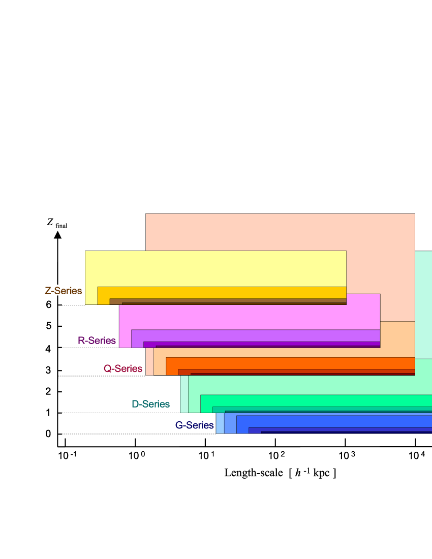
Figure 1: Illustration of the attributes of the simulations analysed in this study. We consider five different box sizes, ranging from $100\,h^{-1}{\rm Mpc}$ to $1\,h^{-1}{\rm Mpc}$. For each box size, a number of simulations have been run, with particle number between $2\times 64^{3}$ and $2\times 324^{3}$. In the diagram, each simulation is represented by a rectangle whose area is proportional to the particle number. The horizontal width of each rectangle gives the spatial dynamic range of the corresponding run, from the gravitational softening scale (left edges) to the box size (right edges), while the lower edge indicates the ending redshift of each run. Numerical parameters of the simulations are listed in Table 1.

Simulation	$L$ [$\,h^{-1}{\rm Mpc}\,$]	Resolution	$m_{\rm DM}$ [$\,h^{-1}{\rm M}_{\odot}\,$]	$m_{\rm gas}$ [$\,h^{-1}{\rm M}_{\odot}\,$]	$z_{\rm start}$	$z_{\rm end}$	$\epsilon$ [$\,h^{-1}{\rm kpc}\,$]
Z1	$1.000$	$2\times 64^{3}$	$2.75\times 10^{5}$	$4.24\times 10^{4}$	199	6	$0.63$
Z2	$1.000$	$2\times 96^{3}$	$8.16\times 10^{4}$	$1.25\times 10^{4}$	199	6	$0.42$
Z3	$1.000$	$2\times 144^{3}$	$2.42\times 10^{4}$	$3.72\times 10^{3}$	199	6	$0.28$
Z4	$1.000$	$2\times 216^{3}$	$7.16\times 10^{3}$	$1.10\times 10^{3}$	199	6	$0.19$
R1	$3.375$	$2\times 64^{3}$	$1.06\times 10^{7}$	$1.63\times 10^{6}$	199	4	$2.11$
R2	$3.375$	$2\times 96^{3}$	$3.14\times 10^{6}$	$4.84\times 10^{5}$	199	4	$1.41$
R3	$3.375$	$2\times 144^{3}$	$9.29\times 10^{5}$	$1.43\times 10^{5}$	199	4	$0.94$
R4	$3.375$	$2\times 216^{3}$	$2.75\times 10^{5}$	$4.24\times 10^{4}$	199	4	$0.63$
Q1	$10.00$	$2\times 64^{3}$	$2.75\times 10^{8}$	$4.24\times 10^{7}$	159	2.75	$6.25$
Q2	$10.00$	$2\times 96^{3}$	$8.16\times 10^{7}$	$1.25\times 10^{7}$	159	2.75	$4.17$
Q3	$10.00$	$2\times 144^{3}$	$2.42\times 10^{7}$	$3.72\times 10^{6}$	159	2.75	$2.78$
Q4	$10.00$	$2\times 216^{3}$	$7.16\times 10^{6}$	$1.10\times 10^{6}$	159	2.75	$1.85$
Q5	$10.00$	$2\times 324^{3}$	$2.12\times 10^{6}$	$3.26\times 10^{5}$	159	2.75	$1.23$
D3	$33.75$	$2\times 144^{3}$	$9.29\times 10^{8}$	$1.43\times 10^{8}$	159	1	$9.38$
D4	$33.75$	$2\times 216^{3}$	$2.75\times 10^{8}$	$4.24\times 10^{7}$	159	1	$6.25$
D5	$33.75$	$2\times 324^{3}$	$8.15\times 10^{7}$	$1.26\times 10^{7}$	159	1	$4.17$
G3	$100.0$	$2\times 144^{3}$	$\;\,2.42\times 10^{10}$	$3.72\times 10^{9}$	79	0	$18.0$
G4	$100.0$	$2\times 216^{3}$	$7.16\times 10^{9}$	$1.10\times 10^{9}$	79	0	$12.0$
G5	$100.0$	$2\times 324^{3}$	$2.12\times 10^{9}$	$3.26\times 10^{8}$	79	0	$8.00$

Table 1: Numerical simulations analysed in this study. Identical cosmological parameters were employed in all the runs, and the same simulation technique for treating star formation and feedback processes was used throughout. For each of our five different box-sizes, we carried out a number of simulations, differing only in mass and spatial resolution. In the table, we list the names of the runs, their particle and mass resolutions, their starting and ending redshifts, and the gravitational softening length $\epsilon$. Simulations with particle resolutions of $2\times 64^{3}$ carry a label ‘1’ in their names, those with $2\times 96^{3}$ are labelled with ‘2’, and so on, up to the $2\times 324^{3}$ runs which are labelled with a ‘5’. The simulations have been carried out with a massively parallel TreeSPH code. Runs at the ‘1’-level were done on 4 processors, and for each higher level, we doubled the number of processors so that level-5 runs were computed on 64 processors.

2.1 Numerical simulations

In this study, we focus on a $\Lambda$CDM cosmological model with parameters $\Omega_{0}=0.3$, $\Omega_{\Lambda}=0.7$, Hubble constant $H_{0}=100\,h\,{\rm km\,s^{-1}\,Mpc^{-1}}$ with $h=0.7$, baryon density $\Omega_{\rm b}=0.04$, and a scale-invariant primordial power spectrum with index $n=1$, normalised to the abundance of rich galaxy clusters at the present day ($\sigma_{8}=0.9$). This “concordance” model provides a good fit to a long list of current cosmological constraints.

All of our smoothed particle hydrodynamics (SPH) simulations were performed in cubic boxes with periodic boundary conditions, employing an equal number of dark matter and gas particles. Besides gravity, the gas particles interact through pressure forces and gain entropy in hydrodynamic shocks. We also follow radiative cooling and heating processes for a primordial mix of hydrogen and helium, using a method similar to Katz et al. (1996). We adopt an external photo-ionising flux that describes radiation from quasars as advocated by Haardt & Madau (1996), leading to reionisation of the Universe at redshift $z\simeq 6$ (for details, see Davé et al., 1999).

Star formation and supernova feedback in the ISM are treated with an effective multi-phase model, which is discussed in full detail in a companion paper by Springel & Hernquist (2002a). In brief, our model assumes that rapidly cooling gas at high overdensity is subject to a thermal instability which leads to the formation of cold clouds embedded in a hot ambient medium. Because the resulting multi-phase structure of the ISM cannot be spatially resolved by available cosmological simulations, we describe the dynamics of the star-forming ISM in terms of a ‘sub-resolution’ model, where coarse-grained averages of fluid quantities are used to describe the medium. In this method, a sufficiently dense SPH fluid element will then represent a satistical mixture of cold clouds and ambient hot gas, with a set of equations governing the mass and energy exchange processes between the phases. In particular, we take the cloud material to be the reservoir of baryons available for star formation. We set the consumption timescale of the gas to match the observed “Kennicutt” law (Kennicutt, 1989, 1998) for the star formation rate in local spiral galaxies. In our formalism, this one free parameter simultaneously determines a threshold density, above which the multiphase structure in the gas and hence star formation is allowed to develop. This physical density is $8.55\times 10^{6}\,h^{2}{\rm M}_{\odot}{\rm kpc}^{-3}$ for all simulations in this study, corresponding to a comoving baryonic overdensity of $7.7\times 10^{5}$ at $z=0$.

In describing star formation numerically, we spawn independent star particles out of the multi-phase medium with mass equal to half the original gas particle mass in a stochastic fashion, as described by Springel & Hernquist (2002a). This avoids any artificial coupling of gas and collisionless stellar material, while the total increase in particle number over the course of a simulation is only modest.

With respect to feedback processes, we assume that massive stars explode as supernovae on a short timescale, releasing their energy as heat to the ambient medium of the ISM. We also assume that supernovae evaporate cold clouds (McKee & Ostriker, 1977), essentially by thermal conduction, thereby “cooling” the ambient hot gas. This process establishes a tight self-regulation cycle for the star-forming ISM. A model quite similar to ours in this respect has been proposed by Yepes et al. (1997). However, our technique differs significantly in the physical parameterisation of cloud evaporation and the star formation timescale, and also in its numerical implementation.

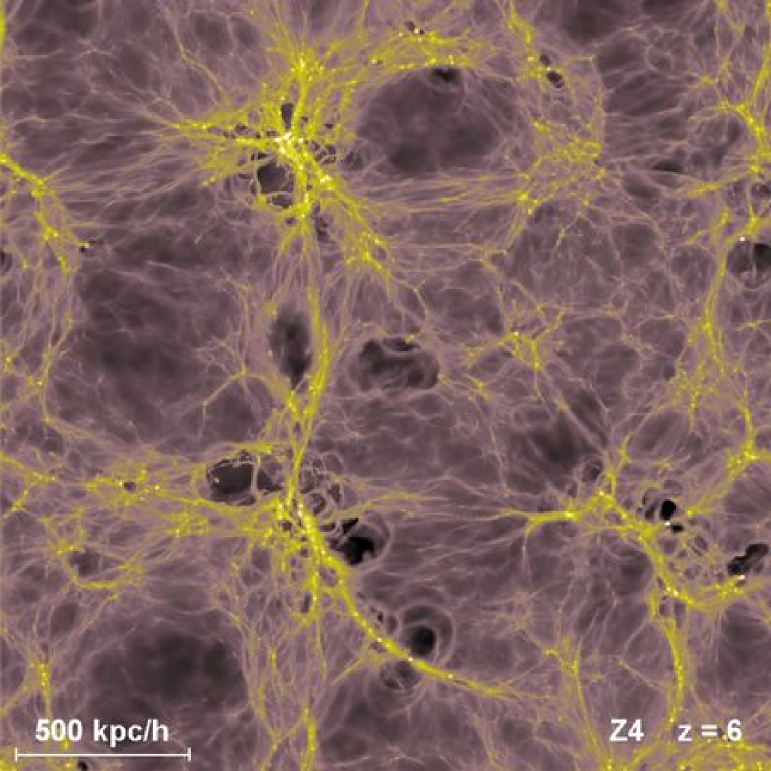
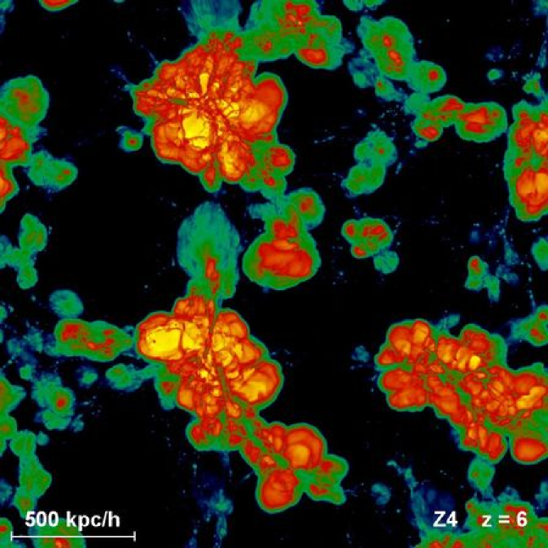
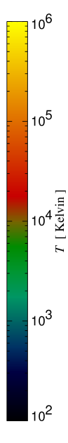
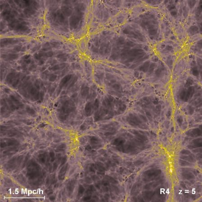
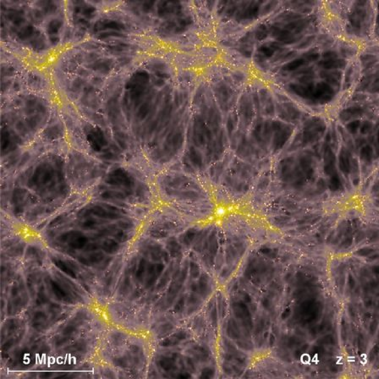
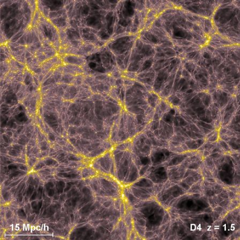
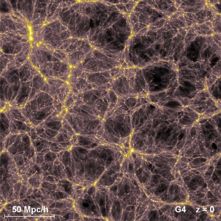
Figure 2: Projected baryonic density fields in slices through a selection of our simulations at various redshifts. In each case, the slice has a thickness equal to $1/5$ of the box-size of the corresponding simulation (see Table 1). The Z4 simulation in the top left has the highest spatial resolution, allowing to identify the hot “bubbles” in the IGM that develop as a result of impinging galactic winds. These bubbles are filled with gas with temperatures up to $10^{6}\,{\rm K}$, as seen in the projected mass-weighted temperature map in the top right.

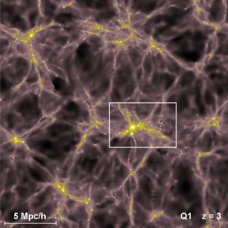
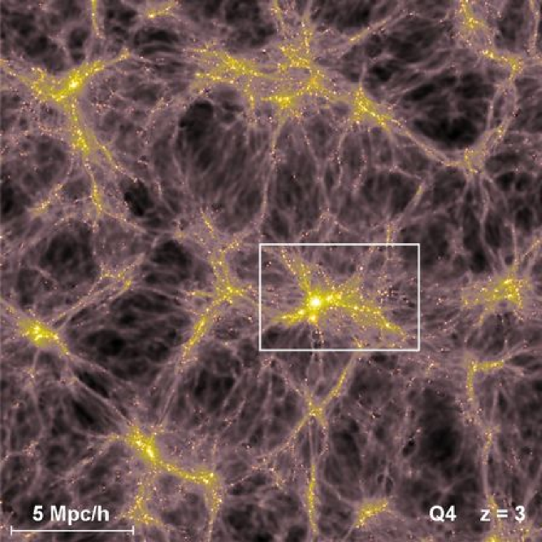
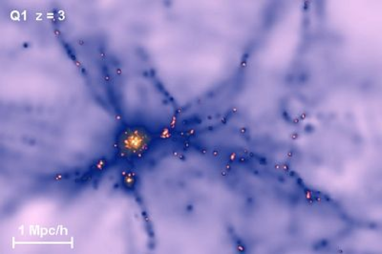
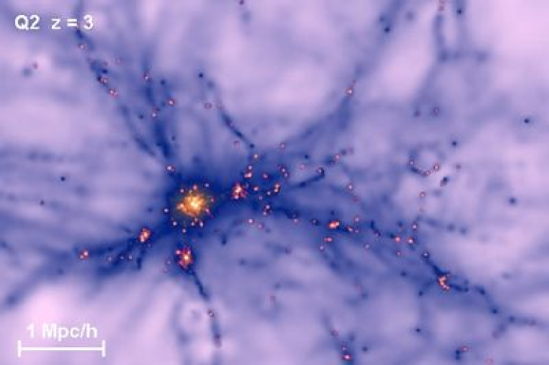
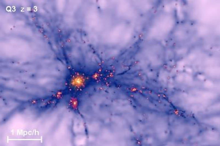
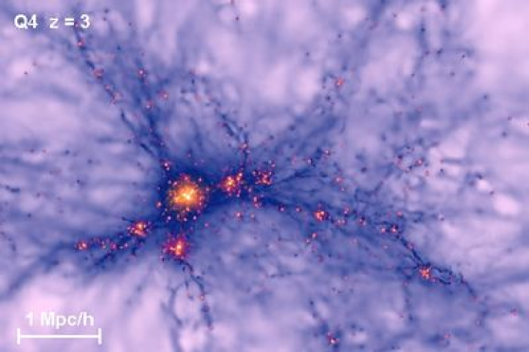
Figure 3: The two panels on top compare the projected baryonic density field in slices through the Q1 and Q4 simulations at $z=3$. It is seen that the runs yield the same large-scale structure, as intended by our method for generating the initial conditions. In the bottom four panels, we zoom in on the region marked by a white rectangle, and show all four members of the Q-Series, where the mass resolution is increasing by a factor of about $40$ along the sequence Q1, Q2, Q3, to Q4. In these panels, the gas density is shown in a blue colour scale, and the density of star particles is in red. The higher resolution runs in the series reproduce the objects previously seen in the low resolution realisations, but they are able to resolve larger numbers of low-mass halos, and they also improve the sampling of structures, giving them a “crisper” appearance. Note, however, that the brightness of the largest objects, as measured by the density of star particles shown in red, appears to be quite similar. This sense of convergence will be quantified more precisely in Section 3.

In addition to this treatment of the multi-phase structure of the ISM, we have included a phenomenological model for galactic outflows in the simulations in our present study. The motivation for this was twofold. On one hand, there is a large body of observational evidence for the ubiquitous presence of such galactic winds (e.g. Heckman et al., 1995; Bland-Hawthorn, 1995; Lehnert & Heckman, 1996; Dahlem et al., 1997; Martin, 1999; Heckman et al., 2000). On the other hand, galactic-scale outflows provide one of the most attractive mechanisms for understanding how the low-density intergalactic medium was chemically enriched with heavy elements, and they might also play a crucial role in the global regulation of star formation, suppressing its overall efficiency to the “low” values suggested by observational estimates of the luminosity density of the Universe. Simulations without strong kinetic feedback invariably overpredict the luminosity density of the Universe due to the high efficiency of gas cooling (e.g. Balogh et al., 2001).

In our fiducial parameterisation of this process, each star-forming galaxy drives a wind with a mass-outflow rate equal to two times its star formation rate, and with a wind-velocity of $v_{w}=484\,{\rm km\,s^{-1}}$. These choices are deliberately “extreme” in the sense that the total kinetic energy of the wind is then of order the energy released by supernovae. Note, however, that these wind parameters are characteristic of the properties of outflows associated with star-forming disks (e.g. Martin, 1999). In addition to the simulations listed in Table 1, which all employed these fiducial values in our wind model, we performed other runs with differing particle number and in boxes of different sizes in which we varied only the intensity of the winds. In this manner, we were able to examine the sensitivity of our conclusions to the presence or absence and strength of the winds.

On a technical level, the winds in the simulations are set up by stochastically selecting gas particles from the star-forming ISM and “adding them” to a wind by modifying their velocity vectors appropriately. While the generation of the wind is hence purely phenomenological, subsequent interactions with surrounding gas are handled properly by our hydrodynamical code. The winds may thus intercept or entrain infalling gas, shock the IGM and even produce hot bubbles within it. Whether or not a wind can escape from a galaxy depends primarily on the depth of the galaxy’s dark matter potential well. Halos with virial temperatures below $\sim 10^{6}\,{\rm K}$ have central escape velocities lower than the wind speed and can lose some of their baryons in an outflow, while more massive halos will contain winds, to the extent that winds become progressively less important for the regulation of star formation in more massive objects.

The fact that winds are expected to be especially important on small mass scales points to one of the main numerical challenges encountered in simulating hierarchical galaxy formation. At high redshift, most of the star formation takes place in low-mass galaxies, which form in abundant numbers as progenitors of more massive systems. Resolving the earliest epochs of star formation, therefore, requires very high mass resolution. However, at low redshift, star formation shifts to progressively more massive systems. At these late times, it is necessary to simulate a large cosmological volume in order to obtain a fair sample of the high-end of the mass function. Obviously, the simultaneous requirements of high mass resolution and large simulation volumes will quickly exhaust any computational resource.

For example, a simulation which attempts to fully resolve star formation in all star forming halos from high-$z$ to the present would have to follow a cosmological volume of $\sim(100\,h^{-1}\,{\rm Mpc})^{3}$, at a mass resolution of about $10^{6}\,h^{-1}{\rm M}_{\odot}$, assuming here for the moment that star formation is restricted to halos of mass larger than $10^{8}\,h^{-1}{\rm M}_{\odot}$, and that a mere 100 SPH particles are sufficient to obtain a reasonably accurate estimate of the star formation rate in a halo. This would require of order $10^{11}$ simulation particles, which is substantially beyond what is currently feasible. Note that unlike in purely gravitational bottom-up growth of structure, feedback processes associated with winds offer the possibility that star formation on small mass scales could influence the gas dynamics on larger scales. Degrading the mass resolution thus may have more problematic consequences than in purely collisionless simulations, because it means that the effects of winds coming from low-mass halos can be lost.

Rather than attempting to resolve the cosmic star formation history in a single calculation, we have, therefore, selected a different strategy. We have simulated a series of cosmological volumes with sizes ranging from $1\,h^{-1}{\rm Mpc}$ to $100\,h^{-1}{\rm Mpc}$ per edge, with intermediate steps at box sizes $3.375$, $10.0$, and $33.75\,h^{-1}{\rm Mpc}$. The smaller boxes are run only to a redshift where their fundamental mode starts to become non-linear. Roughly up to this point, the boxes can at least approximately be taken as a fair sample of a $\Lambda$CDM universe on the scales they are intended to represent.

For each of the box sizes, we have performed a number of runs, varying only the mass and spatial resolution. In particular, we have repeatedly increased the mass resolution in steps of $1.5^{3}$, and the spatial resolution in steps of $1.5$. For example, our lowest resolution run of the $10.0\,h^{-1}{\rm Mpc}$ box had a resolution of $2\times 64^{3}$ particles (‘Q1’-run), which we then stepped up sequentially to $2\times 96^{3}$ (‘Q2’), $2\times 144^{3}$ (‘Q3’), $2\times 216^{3}$ (‘Q4’), and finally to $2\times 324^{3}$ (‘Q5’). In this progression, the mass resolution in the gas is hence improved by a factor $\sim 130$ from $4.2\times 10^{7}\,h^{-1}{\rm Mpc}$ (Q1) to $3.3\times 10^{5}\,h^{-1}{\rm Mpc}$ (Q5), and the 3D spatial resolution by a factor $\sim 5$ from $6.25\,h^{-1}{\rm kpc}$ to $1.23\,h^{-1}{\rm kpc}$. For all simulations which form such a series, we generated initial conditions such that the amplitudes and phases of large-scale waves were identical; i.e. a higher resolution simulation in a series had the same initial fluctuations on large scales as any of the lower resolution fellow members of its series, with additional waves between the old and new Nyquist frequencies sampled from the power spectrum randomly. In this manner, a numerical convergence study within a given series becomes possible which is free of cosmic variance and where an object by object comparison can be made. Note, however, that for different box sizes we have chosen different initial random number seeds, so that they constitute independent realisations.

While the simulations within a given series enable us to cleanly assess the convergence of star formation seen on a given halo mass scale, the dynamic range of even a $2\times 324^{3}$ simulation is too low to identify all the star formation occurring in the Universe. This is where our different box sizes come in. They provide us with a sequence of interlocking scales and epochs, enabling us to significantly broaden the dynamic range of our modeling. For the $1\,h^{-1}{\rm Mpc}$ box of the “Z-series”, we reach mass resolutions of up to $1.1\times 10^{3}h^{-1}{\rm Mpc}$, making it possible to resolve the gas content even in “sterile” dark matter halos which are never able to condense gas in their centres by atomic line cooling. Apart from a putative population III (e.g. Carr et al., 1984; Bromm et al., 1999; Abel et al., 2002), most of them are thus never expected to form stars. At the other end of the spectrum, we resolve rich galaxy clusters in our “G-series” runs, which have a volume $10^{6}$ times larger than the “Z-series”, but a correspondingly poorer mass resolution.

We show a graphical illustration of the numerical simulations analysed in our present study in Figure 1, and give a complete list of their properties in Table 1, together with some important numerical parameters. As a naming convention, the simulations are denoted by a single character that indicates their box size, and a number that gives the particle resolution, from “1” for $2\times 64^{3}$ to “5” for $2\times 324^{3}$. All the simulations were performed on the Athlon-MP cluster at the Center for Parallel Astrophysical Computing (CPAC) at the Harvard-Smithsonian Center for Astrophysics. We used a modified version of the parallel GADGET-code (Springel et al., 2001), and integrated the entropy as the independent thermodynamic variable (Springel & Hernquist, 2002b).

2.2 Slices through the gas density field

In Figure 2, we show projected baryonic density fields for each of our five simulation volumes, illustrating the range of scales encompassed by the simulations. In each case, we visualise the gas density in slices of thickness $1/5$ of the simulation box. To show nearly all of the simulation volume in one projection, we have tilted the slices slightly with respect to the principal axes of the simulation boxes (by $26.6^{\rm o}$ around the $y$-axes, and once more by $26.6^{\rm o}$ around the $x^{\prime}$-axes). Using the periodicity of the volumes, we can then extend the side-length of the projection to $\sqrt{5}$ times the original box size, while approximately avoiding the repetition of structure. In the given representation, we then obtain a thin slice that has exactly the volume of the full simulation box and displays about 90% of its content uniquely. Alternative ways of displaying the “full” simulation would either have to employ several different slices, or would have to project using a slice of thickness equal to the box size itself, leading to a confusing superposition of many structures.

As part of Figure 2, we also show a mass-weighted temperature map of a Z-series run at $z=6$. In the corresponding density map, it is apparent how the first star-forming galaxies drive vigorous outflows that produce hot “bubbles” in the IGM. As seen in the temperature map, these bubbles are filled with gas at temperatures up to $10^{6}\,{\rm K}$. We plan to investigate the impact of these outflows on the IGM in forthcoming work. We note here, however, that the winds are capable of stripping some gas from halos nearby, thereby providing an indirect source of negative feedback in the form advocated by Scannapieco et al. (2001).

In Figure 3, we show a comparison of four simulations within the Q-Series having different mass resolution at redshift $z=3$. It is apparent that better mass resolution leads to more finely resolved structure, and to a larger number of small halos that were previously unresolved. Note, however, that the pattern of large-scale structure and the location of the most massive halos is virtually unchanged, as expected, given our method for constructing the initial conditions for the runs in this series.

2.3 Halo definition

Using our approach, we can directly measure the total star formation rate in a simulation box at each timestep. However, we are interested not only in the cumulative star formation rate normalised to unit comoving volume, but also in the way this rate can be broken up into contributions from various halo mass scales. It should be emphasised that our requirement for the gas to be highly overdense for star formation to occur essentially guarantees that this process is entirely restricted to the centres of dark halos, with no stars forming in the low-density IGM.

In order to identify virialised halos as sites of star formation, we begin by applying a “friends-of-friends” (FOF) group finding algorithm to the dark matter particles, using a fixed comoving linking length equal to $0.2$ times the mean interparticle spacing of the dark matter particles. We restrict the algorithm to the dark matter because it is unclear how one should deal with the varying particle number and particle type used to represent the baryons in the simulations. Owing to the collapse of a large fraction of the gas to very high overdensity, one could introduce biases close to the group detection threshold if a FOF procedure were applied to all particles on an equal footing. It thus seems safer to restrict ourselves to group selection based on dark matter particles alone, which to first order will be unperturbed by the baryonic physics, permitting a selection of the same structures as in an equivalent simulation that followed only dark matter, to a good approximation.

Figure 4: Evolution of the cosmic star formation rate density in the simulations of the Z-, R-, and Q-series. For increasing mass-resolution, there is clearly more star formation resolved at high redshift. However, in every case, there is a certain redshift at which the simulations begin to agree very well. The mass resolution required to reach this convergence point is a function of redshift and becomes increasingly more demanding towards higher redshift.

In a second step, we then associate each gas or star particle with its nearest dark matter particle and discard all groups with fewer than 32 dark matter particles, resulting in our final “FOF catalogue”. Note that Jenkins et al. (2001) have shown that the construction of group catalogues using the same linking length for all cosmologies and redshifts, independent of $\Omega(z)$, leads to mass functions that can be described by a single fitting formula. Group catalogues selected at a constant comoving overdensity with respect to the background, as we do here, are thus easier to interpret than ones obtained by trying to account for the scaling of the virial overdensity with cosmological parameters.

For the analysis of the star formation multiplicity function discussed in Section 4, we will use the FOF catalogues directly, taking the total mass of each group as a “virial” mass, and the sum of the star formation rates of all a group’s SPH particles as the halo’s star formation rate. Following Mo & White (2002), we assign a physical radius to a halo of mass $M$ according to

$$r_{200}=\left[\frac{GM}{100\,\Omega_{m}(z)H^{2}(z)}\right]^{1/3}=\frac{1}{1+z}\left[\frac{GM}{100\,\Omega_{0}H_{0}^{2}}\right]^{1/3},$$ (1)

and a corresponding circular velocity $V_{c}=(GM/r_{200})^{1/2}$. We also define a “virial” temperature as

$$T=\frac{\mu V_{c}^{2}}{2k}\simeq 36\left(\frac{V_{c}}{{\rm km\,s^{-1}}}\right)^{2}\,{\rm K},$$ (2)

where $\mu\simeq 0.6m_{\rm p}$ is the mean molecular weight of the ionised plasma found in halos hotter than $10^{4}\,{\rm K}$.

However, for a comparison of halos on an object-by-object basis between the different runs of a given series, it is advantageous to reduce the noise in the virial mass assignment by using the spherical overdensity algorithm to define the positions and virial radii of halos. To this end, we find the minimum of the gravitational potential of each FOF group, and define the location of the corresponding particle as the halo center. We then grow spheres until they enclose a comoving overdensity of 200 with respect to the mean background density, with the star formation rate of the halo being simply defined as the sum of all the star formation rates of the enclosed SPH particles. In order to match objects between different simulations of a series, we consider the halos of one of the simulations in declining order of mass, and find for each of them the nearest halo in the other simulation. Each halo is only allowed to become a member of one matching pair in this process.

Figure 5: Object-by-object comparison of halos in the Q-Series at redshift $z=3$. We analyse the convergence of the virial mass (top row), the total mass of stars inside the virial radius (middle row), and the total star formation rate within the virial radius (bottom row). In the panels on the left, we plot a direct comparison of measurements for the Q3 and Q4 runs for each of these three quantities. In the panels on the right, we compare results for the 50 most massive halos of all four simulations of the series. Here, the horizontal axes give the number of each halo, in decreasing order of mass. On the vertical axes, we plot for each run the relative deviation of the measured quantity for each halo from the mean of all four runs.

Figure 6: Object-by-object comparison of halos in the R-series at redshift $z=4$. As in Figure 5, we analyse the convergence of the virial mass (top row), the total mass of stars inside the virial radius (middle row), and the total star formation rate within the virial radius (bottom row). In the panels on the left, we plot for each of these three quantities a direct comparison of measurements for the R3 and R4 runs. In the panels on the right, we compare results for the 50 most massive halos of all four simulations of the series, where the horizontal axes simply give the number of each halo, in decreasing order of mass. On the vertical axes, we plot for each run the relative deviation of the measured quantity for each halo from the mean of all four runs.

3 Numerical convergence tests

In this section, we examine the numerical convergence of our simulation results for star formation rates. Figure 4 shows the evolution of the cosmic star formation rate density in the simulations making up the Z-, R-, and Q-Series. In all three cases, the higher resolution simulations predict substantially more star formation at high redshift, but at sufficiently low redshift, the results of the different runs begin to agree quite well.

This behaviour is not surprising. It is clear that simulations with higher mass resolution are able to measure star formation rates in halos of mass smaller than previously resolved. Furthermore, towards higher redshift, the bulk of the star formation shifts to progressively lower mass scales, as expected for hierarchical growth of structure, making it ever more important to resolve low mass objects.

While the convergence between the simulations within a given series at low redshift is encouraging, the disagreement at high redshift implies that none of our simulations alone can be used to reconstruct the star formation history from low to very high redshift. Fortunately, however, the mass resolution needed to achieve convergence at a given redshift is a function of epoch. It becomes increasingly less demanding to do this at lower redshift because at that point increasingly more massive halos dominate the star formation rate. This opens up the possibility of combining simulations on different scales to obtain a composite result for the full history of star formation. This is the approach we use in the present analysis.

However, this strategy can succeed only if we can demonstrate that reliably converged star formation rates can be obtained for individual objects. In Figure 5, we compare halos in the simulations of the Q-series directly with one another, and in Figure 6 we perform the same check for the R-series. In particular, we compare the virial mass, the total mass of stars inside the virial radius, and the total star formation rate within the virial radius, where the properties of halos have been defined using the spherical overdensity algorithm. For each of these three quantities, we show scatter plots that directly compare the $2\times 144^{3}$ and $2\times 216^{3}$ resolutions of the series. In addition, we consider the 50 most massive halos explicitly, and compare all four simulations of the series with one other in the relevant panels.

From this comparison it is clear that for the most massive systems the agreement between the simulations is quite good, without any obvious bias towards lower or higher values of the measured quantities as a consequence of resolution effects. Overall, we consider the comparison to be an important success. It shows that we have indeed formulated a numerically well controlled model for cooling, star formation and strong feedback by galactic outflows. We are not aware that other simulations of cosmological galaxy formation have been demonstrated to pass similar tests with equally good results.

Only close to the resolution limit do we notice a tendency for lower resolution simulations to overpredict the star formation rate. This effect will show up again in the analysis of Section 4. It can be understood as a consequence of the lack of star formation and feedback in unresolved progenitor halos. As a result, a newly formed halo in a low-resolution run will initially have a gas fraction that is essentially equal to the universal baryon fraction, while in a corresponding higher-resolution simulation the gas fraction for the same halo can be lower than this because its progenitors were already able to form stars and lose some of their baryons in galactic outflows.

In summary, the results presented in this section give us confidence that we can obtain meaningful, numerically well-converged results for the star formation rate in a given object at a given epoch. The reason we cannot easily obtain a similarly well-converged result for the cosmic star formation density with a single simulation lies in our failure to obtain a complete sampling of the cosmological mass function together with sufficient mass resolution in one simulation box. A way to circumvent this difficulty will be discussed in the next section.

4 The multiplicity function of cosmic star formation

It is clear that the evolution of the cosmic star formation rate density, $\dot{\rho}_{\star}(z)$, is of fundamental importance to cosmology. At a given epoch, the function $\dot{\rho}_{\star}(z)$ will take on a single value, and, hence, does not describe which objects are responsible for the bulk of star formation occurring at that redshift. To address this issue, we develop the notion of a distribution function of star formation with respect to halo mass; a quantity we will refer to as the “multiplicity function of cosmic star formation”. In defining this property of star forming objects, we implicitly assume that the mass in the Universe can be meaningfully partitioned among gravitationally bound halos, and that star formation is restricted to these halos. The problem thus naturally decomposes into determining the number distribution of halos as a function of mass, the so-called mass function, and then measuring the average star formation rate in halos of a given mass.

We start by briefly reviewing the concept of a cosmological mass function. Let $F(M,z)$ denote the fraction of mass that is bound at epoch $z$ in halos of mass smaller than $M$. It follows that the comoving differential mass function of halos is given by

$$n(M,z)=\frac{\overline{\rho}}{M}\,\frac{{\rm d}F}{{\rm d}{M}},$$ (3)

where $\overline{\rho}$ is the comoving background density, and $n(M,z)\,{\rm d}M$ gives the number density of halos in a mass interval ${\rm d}M$ around $M$.

Figure 7: Mean star formation rate $s(M,z)=\left<\dot{M}_{\star}\right>/M$ in halos, normalised to the halo mass. Each panel shows results for a different redshift. Halos have been binned into logarithmic intervals of width ${\rm dlog}M=0.2$, with the thick lines showing the mean in each bin for several different simulations. The thin line is the spline fit for our best estimate of $s(M,z)$. Vertical lines in each panel mark the mass resolution limits (32 particles) of the FOF catalogues of the simulations shown.

Press & Schechter (1974) proposed that $F(M,z)$ can be approximated by

$$F(M,z)={\rm erf}\left[\frac{\delta_{c}}{\sqrt{2}\,\sigma(M,z)}\right],$$ (4)

where $\delta_{c}=1.686$ is the (linearly extrapolated) critical overdensity for top-hat collapse, and $\sigma(M,z)$ describes the rms fluctuations of the linearly evolved density field at redshift $z$, smoothed by a top-hat sphere that just encloses a background mass equal to $M$. The variance of the filtered density field is given by

$$\sigma^{2}(M,z)=\int P_{z}(k)\,|W_{R}(k)|^{2}\,{\rm d}^{3}k,$$ (5)

where $W_{R}(k)=3j_{1}(kR)/(kR)$, $R=[3M/(4\pi\overline{\rho})]^{1/3}$, and $P_{z}(k)$ denotes the power spectrum linearly evolved to redshift $z$.

Overall, the Press-Schechter (PS) mass function provides a surprisingly good description of numerical N-body simulations of non-linear gravitational growth of structure. However, recent high precision work has also clearly established that there are non-negligible discrepancies between PS theory and simulations. The PS formula overpredicts the abundance of halos at intermediate mass-scales, and underpredicts the abundance of both low and high mass halos. This deficiency has led to the development of more accurate fitting formulae.

In particular, Sheth & Tormen (1999) have found a significantly improved parameterisation, based on an excursion set formalism. The Sheth & Tormen (1999) mass function can be expressed as

$$n(M,z)=\frac{\overline{\rho}}{M^{2}}\,\frac{{\rm d}\ln\sigma^{-1}}{{\rm d}\ln M\;\,\,}\,f(\sigma),$$ (6)

where

$$f(\sigma)=A\sqrt{\frac{2a}{\pi}}\left[1+\left(\frac{\sigma^{2}}{a\delta_{c}^{2}}\right)^{p}\right]\frac{\delta_{c}}{\sigma}\exp\left(-\frac{a\delta_{c}^{2}}{2\sigma^{2}}\right),$$ (7)

with $A=0.3222$, $a=0.707$, and $p=0.3$. Sheth et al. (2001) and Sheth & Tormen (2002) also showed that this modified mass function can be understood in terms of an extension of the excursion set formalism that allows for ellipsoidal collapse.

In a comprehensive analysis of a number of N-body simulations, Jenkins et al. (2001) showed that the Sheth & Tormen mass function works remarkably well over at least four decades in mass. In addition, the quality of the fit is nearly independent of cosmology, power spectrum, and epoch, provided that $\delta_{c}=1.686$ is taken in all cosmologies and the mass function is measured at fixed comoving overdensity, independent of $\Omega(z)$. If instead the expected cosmological scaling of the virial overdensity for top-hat collapse is used in the construction of the halo catalogue itself, the universality of the mass function is slightly broken. It is clearly preferable to have a universal mass function for all cosmologies; hence, we have identified our halos at fixed comoving overdensity.

The mass function may also be expressed in terms of the multiplicity function $g(M)$ of halos, which we define as

$$g(M)=\frac{{\rm d}F}{{\rm d}\log M}.$$ (8)

This quantity gives the fraction of mass that is bound in halos per unit logarithmic interval in mass. In a plot of $g(M)$ versus $\log M$, the area under the curve then directly corresponds to the fraction of mass bound in the respective mass range. For the Sheth & Tormen mass function, the multiplicity function is given by

$$g(M)=f(\sigma)\,\frac{{\rm d}\ln\sigma^{-1}}{{\rm d}\log M\,}.$$ (9)

We now introduce a similar quantity for the cosmic star formation rate density. Let us define

$$s(M,z)=\frac{\left<\dot{M}_{\star}\right>}{M}$$ (10)

to be the mean star formation rate of halos of mass $M$ at epoch $z$, normalised to the masses of the halos. With this normalisation, $s(M,z)$ makes possible a direct comparison of the mean efficiency of star formation between halos of different mass. Much of the effort of the numerical work of this paper is focused on trying to measure this function from our set of simulations over a broad range of mass scales and redshifts.

Once $s(M,z)$ is known, the cosmic star formation rate density can be computed from

$$\dot{\rho}_{\star}(z)=\overline{\rho}\int s(M,z)\,g(M,z)\,{\rm d}\log M.$$ (11)

We call the function

$$S(M,z)=s(M,z)\,g(M,z)$$ (12)

the multiplicity function of star formation, in analogy to the multiplicity function of the halo mass distribution.

There are a number of advantages to factoring the star formation rate in the manner suggested by equations (11) and (12). First, a plot of $S(M)$ versus $\log M$ cleanly illustrates which halo mass scales are responsible for the bulk of star formation occurring at a given epoch. Second, even if a numerical simulation can provide an accurate measurement of $s(M,z)$ over an extended range of mass scales, it is difficult if not impossible for any simulation to accurately determine the mass function $g(M,z)$ at the same time. This is because accurate measurements of $s(M,z)$ primarily require high mass resolution, which typically necessitates the use of rather small simulation volumes, resulting in a poor representation of the cosmological mass function. In particular, at the high-mass end, one will typically suffer from completeness problems. However, the analytic form of the mass function can then be used to compute an estimate of the expected star formation density in a simulation in which the mass function was sampled precisely. Provided that $s(M,z)$ varies sufficiently slowly with $M$, it may be also be possible to extrapolate $s(M,z)$ into regions not well probed by the simulation, although this procedure clearly requires some caution.

Figure 8: Normalised star formation rate $s=\left<\dot{M}_{\star}\right>/M$ in a series of small test simulations of isolated NFW halos at $z=0$. The halos have been set-up in virial equilibrium with masses between $10^{7}$ and $10^{15}\,h^{-1}{\rm M}_{\odot}$, all with a self-similar structure initially. We have then evolved them with the same model for cooling, star formation, and feedback as in the cosmological simulations, and measured their star formation rates at a time $2.5\,{\rm Gyr}$ after the simulations were started. Despite the simplicity of these simulations, a qualitatively similar behaviour as for the function $\tilde{s}_{z}(T)$ measured from the full cosmological simulations is observed. Note in particular the suppression of star formation in halos with virial temperatures below $10^{6}\,{\rm K}$ (where galactic winds can escape), the complete absence of star formation for virial temperatures below $10^{4}\,{\rm K}$ (due to the absence of radiative cooling mechanisms), and the peak at a temperature $\sim 10^{7}\,{\rm K}$ (due to the decline of the efficiency of cooling flows at still higher temperatures).

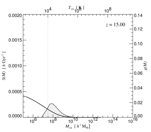
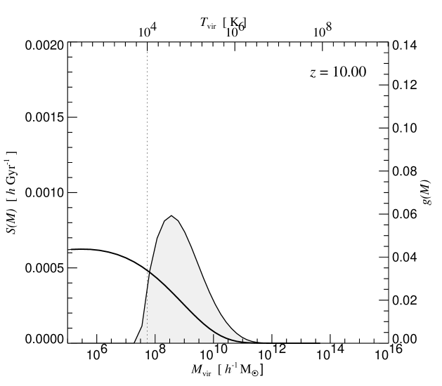
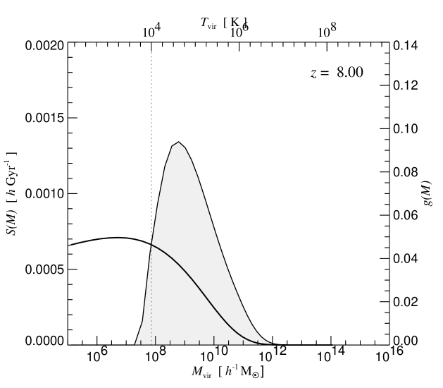
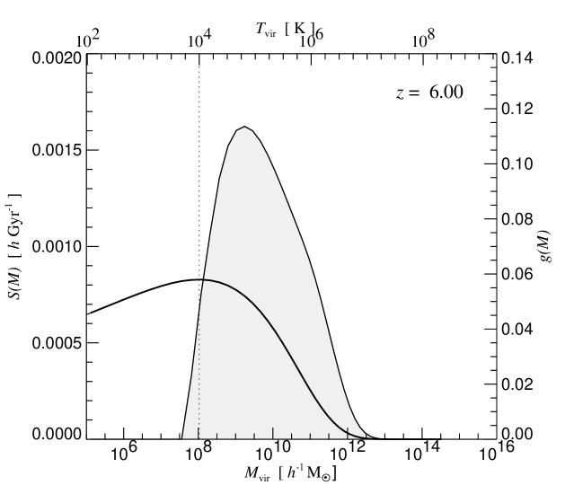
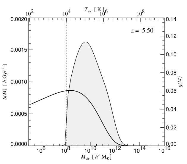
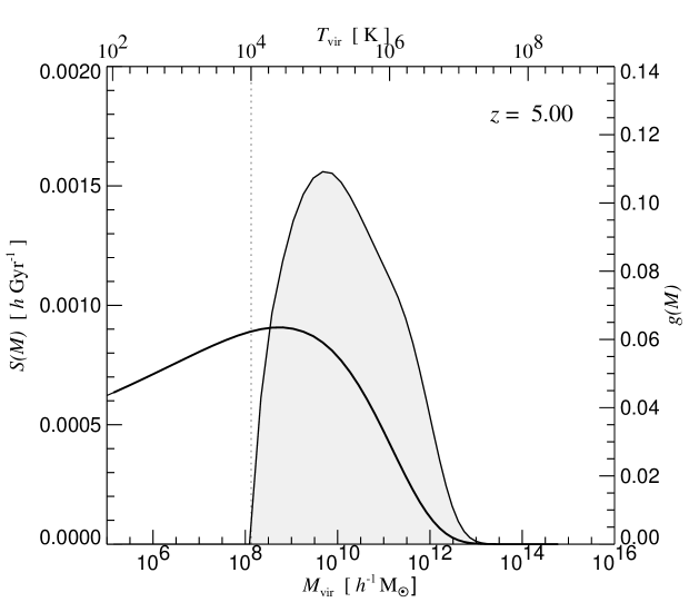
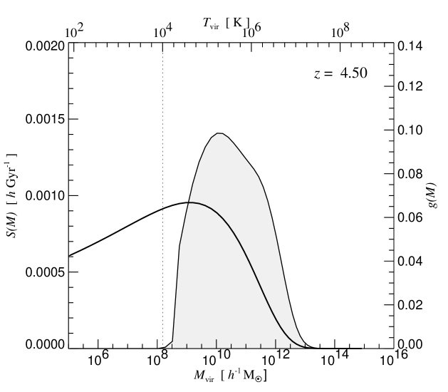
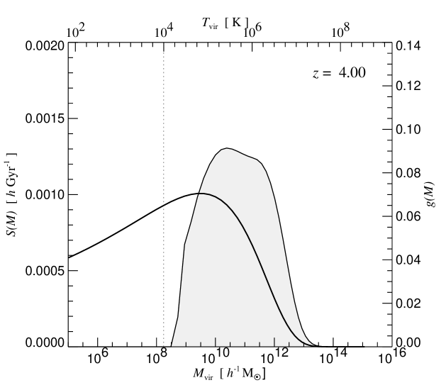
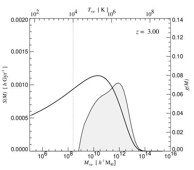
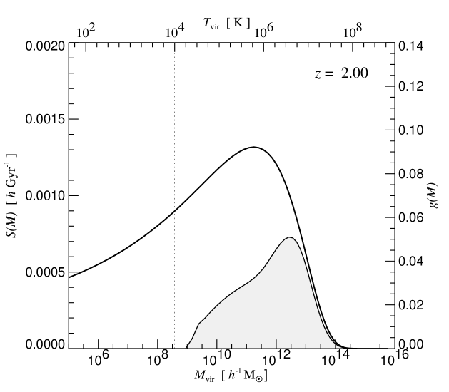
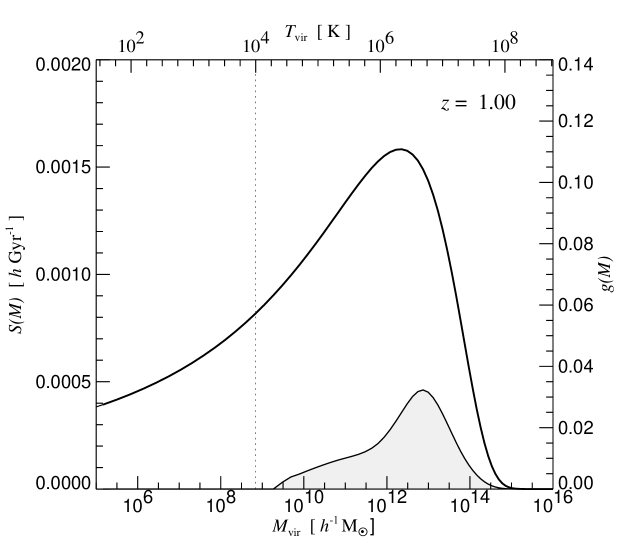
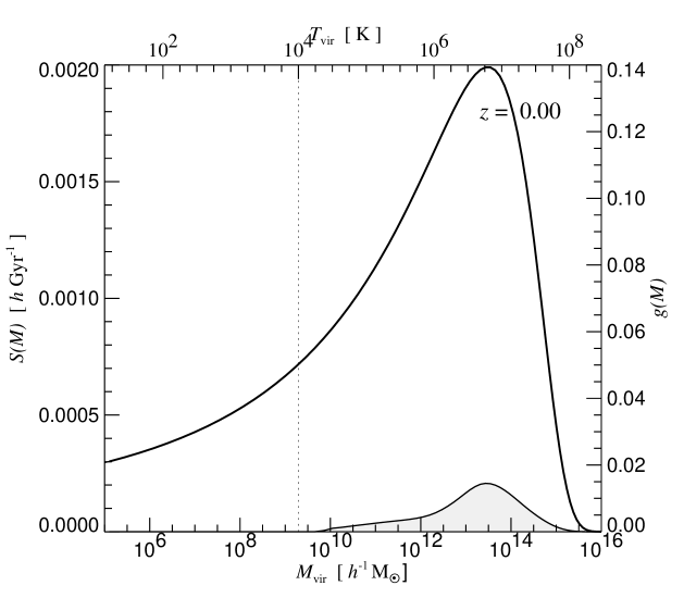
Figure 9: Multiplicity function of star formation (shaded) as a function of redshift. This quantity is defined as the product of our measurements for $s(M,z)=\left<\dot{M}_{\star}\right>/M$ with the Sheth & Tormen multiplicity function (solid line) for the bound mass in halos. On the top axes of each panel, we give the corresponding virial temperature scale at each epoch, and we indicate the temperature $10^{4}\,{\rm K}$ by a dotted vertical line.

In Figure 7, we show examples of our measurements of $s(M,z)$ from the simulations. At each redshift, we have binned the halos by mass in logarithmic intervals of width ${\rm dlog}M=0.2$, and computed the arithmetic mean of $\dot{M}_{\star}/M$ for each bin. Using the different simulation results available at each redshift, we then fitted a smooth spline function to our results, which represents our best estimate for $s(M,z)=\left<\dot{M}_{\star}\right>/M$. Note that this is not an entirely straightforward process, as a cursory look at the example measurements in Figure 7 shows.

In particular, simulations that cannot resolve all star forming halos above $T_{\rm vir}\simeq 10^{4}\,{\rm K}$ exhibit a biased result at their resolution limit, in the form of an overestimate of $\left<\dot{M}_{\star}\right>/M$. This is because star formation and feedback in halos of still lower mass were missed in these simulations, so the gas fraction has not been reduced yet by galactic outflows in progenitor halos, unlike in simulations at higher mass resolution. There is hence a “compensation effect” in simulations with poor mass resolution. Some of the star formation missed in unresolved halos is shifted towards the first generation of halos that are resolved, partly making up for what was missed.

Obviously, these biases complicate the measurement of $s(M,z)$ considerably, particularly if only a single redshift is considered. However, we are aided by our large set of simulations of different mass resolution, and also by the fact that $s(M,z)$ appears to maintain its shape surprisingly well when expressed as a function of virial temperature, i.e. when $s(M,z)$ is factored as

$$s(M,z)=q(z)\,\tilde{s}_{z}(T_{\rm vir}),$$ (13)

where $T_{\rm vir}$ is the virial temperature of a halo of mass $M$ at redshift $z$. Here $q(z)$ describes an “amplitude” function, and $\tilde{s}_{z}(T)$ is the “shape” of the normalised star formation rate as a function of virial temperature. To a very good approximation, this shape appears to be independent of epoch, i.e. all the redshift dependence can be absorbed into the global scaling parameter $q(z)$. Only at virial temperatures between $\simeq 10^{4}\,{\rm K}$ and $\simeq 5\times 10^{4}\,{\rm K}$ is this not fully true. Here, the photoionising background reduces the efficiency of star formation during reionisation, which we take into account as a residual dependence of $\tilde{s}_{z}(T)$ on redshift.

Using our large set of simulations at many different output redshifts, we find that there is a rapid rise of $\tilde{s}_{z}(T)$ at the onset of star formation, followed by a shallow increase towards more massive halos. At a temperature of about $10^{6}\,{\rm K}$, $\tilde{s}_{z}(T)$ begins to increase more rapidly. This scale is very likely related to the velocity of the galactic winds that star forming regions can generate in our simulations. For halos with virial temperatures above $10^{6}\,{\rm K}$, winds are expected to be unable to flow out into the IGM. This renders the feedback induced by outflows much less efficient. Finally, at a temperature of about $10^{7}\,{\rm K}$, the rate of star formation begins to fall again, presumably because halos start to experience less efficient cooling flows. Note that the peak can only be explored at low redshift, when the corresponding halos have actually formed. At high redshift, we formally assume that it still exists in our parameterisation of $\tilde{s}_{z}(T)$, but whether or not this is actually true is unimportant, because the halo multiplicity function vanishes at the corresponding mass scales at high redshift, so that no contribution to $\dot{\rho}_{\star}(z)$ arises.

We have also carried out a number of small test simulations of isolated halos to see whether the behaviour of $\tilde{s}_{z}(T)$ measured in the cosmological simulations can be qualitatively recovered by studying isolated systems. To this end, we set up a series of isolated NFW-halos (Navarro et al., 1996, 1997) consisting of dark matter and gas, with the gas initially being distributed like the dark matter. Initial particle velocities and gas temperatures were assigned so that the halos begin in virial equilibrium to very good approximation, with concentration $c=10$, baryon mass fraction $f_{b}=0.13$, and spin parameter $\lambda=0.1$. We set up 17 halos with total masses spaced logarithmically between $10^{7}\,h^{-1}{\rm M}_{\odot}$ and $10^{15}\,h^{-1}{\rm M}_{\odot}$, using 40000 gas and 80000 dark matter particles, and with physical sizes corresponding to their expected extent at $z=0$. We then evolved these halos in isolation using the same model for cooling, star formation, and feedback as used in the cosmological runs, except that there was no ionising UV background. Note that the initial conditions for all the halos were identical except for an overall scaling, i.e. without the physics of cooling and star formation they would evolve in a self-similar manner.

In Figure 8, we show the normalised star formation rate in these models at a time $t=2.5\,{\rm Gyr}$ after the simulations have been started. At this point, the halos form stars at an approximately steady rate, with the initial rapid phase of disk formation already being largely completed. We expect that a measurement at this time should be qualitatively similar to $\tilde{s}_{z}(T)$ inferred from the cosmological simulations, and this is indeed the case. Note, in particular, the interesting maximum at a temperature of around $10^{7}\,{\rm K}$. More massive halos exhibit a lower star formation rate because their cooling flows are less efficient when normalised to the total gas content of the halo. These results demonstrate that we are able to faithfully match the properties of individual forming galaxies in our cosmological volumes.

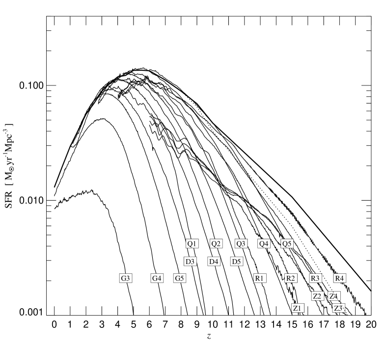
Figure 10: Evolution of the comoving cosmic star formation rate density in all of our simulations on a common plot. Individual runs are labelled at the bottom. It is seen that the collection of runs forms a common “envelope”, with each simulation of low mass-resolution eventually breaking away from the envelope at sufficiently high redshift. A simulation may also underpredict the cosmic star formation density when its volume is too small to resolve a fair sample of the high end of the mass spectrum of halos expected at the given epoch. This is the case for the Z-series at “low” redshifts of $z<15$. At these epochs, the star formation is dominated by the rarest massive objects, of which the Z-series does not contain a proper number. Interestingly, the common envelope formed by the simulations is very well reproduced if we multiply our measurement for the average star formation rate in halos of a given mass, $s(M,z)=\left<\dot{M}_{\star}\right>/M$, with the Sheth & Tormen mass function, and integrate the resulting multiplicity function to obtain $\dot{\rho}_{\star}(z)$. This result is shown as the bold line, and may be viewed as our prediction for the star formation history, corrected for incomplete sampling of the halo mass function. The dotted line shows the result of this computation if the Press & Schechter mass function is used instead at high redshift.

It is also interesting to note that the “amplitude” $q(z)$ measured in the cosmological simulations scales approximately as $q(z)\propto(1+z)^{3}$ over an extended redshift interval between $z\sim 1-8$, with the scaling being somewhat slower at very low and very high redshift. This result can be understood if at intermediate redshifts the halos are modelled as self-similar, with the star formation rate following the cosmological scaling of the cooling time.

In Figure 9, we show our final result for the multiplicity function of the cosmic star formation rate density. Following equation (12), we have defined it as the product of our spline fits for $s(M,z)$ obtained from our full set of simulations with the Sheth & Tormen multiplicity function for the $\Lambda$CDM model. Note that in the representation of Figure 9, the area under the curve of the multiplicity function (shaded) is proportional to the star formation rate density. In each redshift panel, we also show the multiplicity function of the mass distribution in bound halos at the corresponding epoch. It is seen how the history of $\dot{\rho}_{\star}(z)$ arises by the interplay of two opposing trends. The gradual shift of the mass multiplicity function towards higher mass scales leads to an ever increasing fraction of mass bound in star-forming halos with virial temperatures well above $10^{4}\,{\rm K}$. On the other hand, star formation in halos of a given mass becomes less efficient with time because of the decline of the mean density within halos as a result of cosmic expansion. Together, these effects then produce a maximum of the star formation rate at an intermediate epoch, with a fall-off from there towards both low and high redshifts.

5 Evolution of the cosmic star formation rate density

5.1 Numerical results

In Figure 10, we show the evolution of the cosmic star formation rate per unit comoving volume, as directly measured from all of our simulations. Interestingly, the collection of runs appears to describe an “envelope”, which we tentatively interpret as the result for a fully converged numerical simulation with good sampling of the entire cosmological mass function. Simulations of low mass-resolution eventually break away from this envelope towards high redshift. The poorer the resolution, the lower the redshift at which this occurs. This trend is consistent with our expectations developed in Section 4, based on the joint analysis of the multiplicity functions of star formation and mass.

Note, however, that a simulation may also underpredict the cosmic star formation rate density at a given epoch when its volume is too small to contain a fair sample of the high end of the mass function. This is the case for the Z-series at “low” redshifts of $z<15$. At these epochs, the star formation rate density is dominated by the rarest objects in the exponential tail of the mass function, which the Z-series does not properly sample, owing to insufficient volume.

It is now interesting to see whether the common envelope traced out by the simulations is reproduced if we multiply our measurements for the average star formation in halos of a given mass, $s(M,z)=\left<\dot{M}_{\star}\right>/M$, with the Sheth & Tormen multiplicity function, and integrate to obtain $\dot{\rho}_{\star}$ using equation (11). The result we obtain from this procedure is the bold line drawn in Figure 10. The good agreement between this curve and the “envelope” from the individual simulations indirectly shows that the Sheth & Tormen mass function provides an adequate description of the halo abundance in our simulations. Only at very high redshift do the simulations fall slightly short of the expectation from the analytic mass function. In this regime, the cosmic mean of the star formation rate density is dominated by very rare objects in the exponential tail of the mass function, making it difficult to obtain a representative sample in a small simulation volume. It is also possible that the Sheth & Tormen multiplicity function becomes less accurate at these high redshifts, where it is largely untested. In fact, if we use the Press & Schechter mass function to integrate the expected star formation density, we obtain the result indicated by the dotted line in Figure 10, which lies substantially below the Sheth & Tormen result at very high redshift. At intermediate redshifts of around $z\sim 10$, the difference essentially vanishes, while at lower redshift, the Press & Schechter result lies higher. This is consistent with Jang-Condell & Hernquist (2001), who found that the halo abundance measured in collisionless simulations at redshift $z=10$ matches the Press & Schechter prediction quite well. Overall, the results in Figure 10 give us confidence that we can identify our measurements of $s(M,z)$ from our simulations convolved with the Sheth & Tormen mass function as the best estimate for the expected star formation rate density in fully resolved simulations of essentially arbitrarily large volume. In the remainder of our analysis we will therefore adopt this composite result as the prediction of our numerical simulations.

Interestingly, we have found that the composite simulation result can be remarkably well-fitted by a double exponential of the form

$$\dot{\rho}_{\star}(z)=\dot{\rho}_{m}\,\frac{\beta\exp\left[\alpha(z-z_{m})\right]}{\beta-\alpha+\alpha\exp\left[\beta(z-z_{m})\right]},$$ (14)

where $\alpha=3/5$, $\beta=14/15$, $z_{m}=5.4$ marks a break redshift, and $\dot{\rho}_{m}=0.15\,{\rm M}_{\odot}{\rm yr}^{-1}{\rm Mpc}^{-3}$ fixes the overall normalisation. In Figure 11, we compare this fit to our measurement, and find it to be accurate to within $\simeq 15\%$ in the range $0\leq z\leq 20$. We suspect that the variation of the parameter values of the fitting function with cosmological parameters can be understood in terms of simple scaling arguments, an idea that we will pursue further elsewhere.

5.2 Comparison with observational measurements

In Figure 12, we compare a variety of direct observational constraints of the cosmic star formation rate density with our prediction. For this comparison, we have used a compilation of observational data put together by Somerville et al. (2001), who have also computed corrections for incompleteness, and for the $\Lambda$CDM cosmology if appropriate. In addition, we have applied a uniform dust correction of 0.33 in the log to UV-data at high redshift. It should be kept in mind that observing the cosmic star formation density is not only intrinsically challenging, but also involves quite substantial corrections that make it difficult to assess measurement uncertainty.

Figure 11: Cosmic star formation rate density of our composite simulation result (thick line) compared to the analytic fit (thin line) given in equation (14). The accuracy of the double-exponential fit is better than about $15\%$ over the full redshift range $0\leq z\leq 20$.

In our model, the star formation rate peaks in the redshift range $z\sim 5-6$. This is substantially higher than the peak at $z\sim 1-2$ suggested by the early work of Madau et al. (1996), a result which however was probably severely affected by dust corrections unknown at the time. The newer high-redshift points of Steidel et al. (1999) and Hughes et al. (1998) actually appear to be consistent with our prediction. Also, our simulations are in good agreement with data for the Local Universe from Gallego et al. (1995) and Treyer et al. (1998), but not Gronwall (1999).

However, if we assume that all the data points are unbiased, our result seems low compared to the “average” at redshifts around $z\sim 1$. These high observational results at $z\sim 1$ suggest a very rapid decline of the star formation rate towards the present epoch. For example, Hogg (2001) analysed the diverse set of available data from the literature and estimates $\dot{\rho}_{\star}\propto(1+z)^{\beta}$ with $\beta=3.1\pm 0.7$. Such a steep evolution was first suggested by Lilly et al. (1996), based on an analysis of the Canada-France Redshift survey. Our model prediction clearly evolves more slowly than this estimate.

On the other hand, the more gradual decline of star formation found by us is in better agreement with the result of Cowie et al. (1999). Recently, this group has been able to substantially increase their observational sample of multicolour data and spectroscopic redshifts from the Hawaii Survey Fields and the Hubble Deep Field, allowing a selection based on rest-frame UV up to a redshift of $z=1.5$. Wilson et al. (2002) confirm a shallow evolutionary rate of $(1+z)^{1.7\pm 1.0}$ over this redshift range from this new data. We think our results for the star formation history are broadly consistent with the data, given the current level of uncertainty in the observational determinations. Note that a proper treatment of metal-line cooling has the potential to increase our star formation estimate at low redshift, as discussed by Hernquist & Springel (2002). This could eliminate a potential deficit of star formation at low redshift in our model if future observational improvements confirm this suggestion of the present data.

It is also interesting to compare our prediction with other theoretical studies of the cosmic star formation history. Baugh et al. (1998) have analysed the cosmic star formation history using semi-analytic models. They find a rapid decline of star formation at low redshift, with a peak occurring around $z\sim 2$, clearly quite different from the history found here. Their result implies that 50% of the stars form after $z\simeq 1$ in their low-density model, with very little star formation occurring at high redshift. Fewer than 10% of the stars are formed beyond redshift $z>3$ according to their picture. This tendency for the bulk of stars to be formed at relatively low redshift is not found in our simulation result, as we will discuss in more detail in Section 6.

Somerville et al. (2001) used a similar technique to predict the history of star formation from the present to a redshift of $z=6$. They actually find a star formation history resembling ours, but only for their “collisional starburst” model. Their “constant efficiency quiescent” model appears to predict at least an order of magnitude less star formation for redshifts higher than 5 than found in our simulations. This is quite curious. While our simulations are in principle capable of following the triggering of intensified star formation as a result of gas inflow in mergers, we doubt we presently have sufficient numerical resolution to follow this process faithfully, particularly at high redshift. It seems more likely that our simulations have such high star formation rates because our intrinsic, “quiescent” mode of star formation is very efficient at high redshift.

In the numerical simulation of Nagamine et al. (2001), the cosmic star formation rate rises quickly from the present epoch to about $z\sim 1$, and then continues to increase monotonically but slowly towards high redshift, staying nearly constant between redshifts 2 and 7, the highest redshift for which they cite results. The peak of the star formation rate therefore appears to occur beyond redshift 7 in their model. In earlier work by Nagamine et al. (2000), a peak at $z\simeq 2$ was observed, but they also showed in this study that this first result was strongly dependent on numerical resolution and had not converged yet; doubling the box size from $50$ to $100\,h^{-1}{\rm Mpc}$ and hence lowering the spatial resolution by a factor of two also lowered the star formation density by about a factor of two.

Figure 12: Cosmic star formation history for our composite simulation result (solid line) compared to data. Symbols mark various observational results, here largely adopted from a recent compilation by Somerville et al. (2001), who also applied corrections for incompleteness and converted to a $\Lambda$CDM cosmology, where appropriate. The data originate from Gallego et al. (1995, filled triangle), Gronwall (1999, thin diagonal cross), Treyer et al. (1998, open triangle), Tresse & Maddox (1998, hollow circle), Lilly et al. (1996, filled stars), Connolly et al. (1997, filled squares), Madau et al. (1998, filled circles), Pascarelle et al. (1998, empty squares), Flores et al. (1999, empty stars), Cowie et al. (1996, filled diamonds), Hughes et al. (1998, filled hexagon), Steidel et al. (1999, hollow hexagons). Following Somerville et al. (2001), we also applied a uniform dust correction factor of 0.33 in the log to the 1500 Angstrom UV-points at $z>2$ of Madau et al. (1998), Steidel et al. (1999) and Pascarelle et al. (1998). Note: In the published version of this figure, all observational data points were erroneously drawn by a factor $1/h=1.43$ too high.

Ascasibar et al. (2002) also investigated the cosmic star formation history by means of hydrodynamic mesh simulations. In fact, they used a multi-phase model quite similar in spirit to the one employed here, although theirs differs substantially in the details of its formulation. Similar to Nagamine et al. (2001), their $\Lambda$CDM models predict a nearly constant star formation density over an extended redshift range, but Ascasibar et al. (2002) find a peak at a low redshift of about $z=1.0-1.5$, with a gradual decline towards higher redshift.

In both of these numerical studies, hydrodynamical mesh-codes have been used which have severe difficulty in resolving star-forming regions with the appropriate size and density, despite the high accuracy these numerical techniques have for the hydrodynamics of gas at moderate and low overdensity. We suspect that this might make it relatively difficult to achieve numerical convergence for the star formation density using this approach. We expect our Lagrangian simulation technique to offer better behaviour in this respect, although it can suffer from (different) numerical limitations (e.g. Weinberg et al., 1999; Pearce et al., 2001; Springel & Hernquist, 2002b), depending on details of its implementation.

Finally, we comment on the behaviour of the cosmic star formation rate density at the epoch of reionisation. In our simulations, an externally imposed UV background radiation of the form used by Davé et al. (1999) starts to reionise the Universe at redshift $z=6$. However, we do not find the distinctive drop of the cosmic star formation rate at the epoch of reionisation predicted by Barkana & Loeb (2000). From Figure 9, we see that after the epoch of reionisation, the UV background efficiently suppresses star formation in halos of virial temperatures up to $\sim 5\times 10^{4}\,{\rm K}$, but the halos in this mass range do not make a very significant contribution to the total star formation rate density. At the epoch of reionisation at redshift $z=6$, the bulk of star formation has already shifted to higher mass scales, so that photoionisation reduces the total star formation rate by only 10-20%. For a higher reionisation redshift, we would expect to see a stronger effect, however. Note that a number of semi-analytic studies of photoionisation “squelching” of star formation in dwarf galaxies (Bullock et al., 2000, 2001; Barkana & Loeb, 2000; Somerville, 2002; Benson et al., 2002a, b) have assumed a relatively strong depletion of the gas fraction, and a corresponding reduction of the star formation rate, in halos of virial temperatures of up to $10^{5}\,{\rm K}$. Our numerical results suggest that this effect may have been overestimated in these studies.

5.3 The cosmic density in stars

An immediate corollary of our star formation history is the total density of stars and stellar remnants we expect to have formed by the present epoch. We find $\Omega_{\star}=0.004$ for this quantity in units of the critical density, corresponding to $\sim$10% of all baryons being locked up in long-lived stars. This is substantially lower than is typically found in hydrodynamic simulations that do not include strong feedback processes, and this low value brings us into better agreement with observational estimates of $\Omega_{\star}$ based on the local luminosity density.

Cole et al. (2001) used the 2dF and 2MASS catalogues to constrain the K- and J-band luminosity functions. For a $\Lambda$CDM cosmology, they find a total density in stars of $\Omega_{\star}=(1.6\pm 0.24)\times 10^{-3}h^{-1}$ for a Kennicutt IMF, and $\Omega_{\star}=(2.9\pm 0.43)\times 10^{-3}h^{-1}$ for a Salpeter IMF (see also Balogh et al., 2001). Note that for the baryon density of $\Omega_{b}=0.04$ we adopted (motivated by constraints from big bang nucleosynthesis), this means that only between 5-12% of the baryons appear to be locked up in stars. Similarly low values are found using optical data. For example, Fukugita et al. (1998) estimated the global budget of baryons in all states, based on a large variety of data, and found $\Omega_{\star}=2.45^{+1.7}_{-1.0}\times 10^{-3}h^{-1}$, corresponding to about 17% of the sum of all baryons they were able to detect. This sum amounted to $\Omega_{b}=0.021\pm 0.007$ in their study, falling somewhat short of current nucleosynthesis constraints. However, this difference can be attributed to a state of baryons unaccounted for in their study, the reservoir of warm-hot gas in the IGM that is seen in simulations (Cen & Ostriker, 1999; Davé et al., 2001), but which is difficult to detect in either absorption or emission. This lowers the relative contribution of stars in the baryon budget, leading to values in agreement with the K-band results. Note that our simulation result of $\Omega_{\star}=2.8\times 10^{-3}h^{-1}$ is consistent with these constraints.

Figure 13: Cumulative star formation as a function of lookback time (top), or redshift (bottom). In both panels, we plot the fraction of stars that have formed by a given lookback time or redshift, respectively, with the broken lines indicating 10%, 50%, and 90% percentiles. The arrow marks an upper limit by Baldry et al. (2002) for the relative fraction of stars that may at most have formed in the redshift range $z>1$. We provide a tabulated form of the data in this figure in Table 2.

Figure 14: Mean (solid) and median (dashed) ages of stars that have formed up to a certain epoch $z$. The dotted line shows the age of the universe as a function of redshift. For redshifts higher than $z\simeq 2.5$, the global stellar population is quite young, with a mean age below 1 Gyr. However, after this epoch, the mean age nearly increases as rapidly as the age of the Universe itself, because the star formation rate density is rapidly declining towards low redshift. As a result, the mean age of all stars is about 9 Gyr at the present epoch.

6 When and where stars form

In this section, we examine the cumulative history of cosmic star formation, as predicted by our composite simulation result. This is shown in Figure 13, both as a function of redshift and lookback time. Interestingly, already half the stars have formed by redshift $z\sim 2.14$ in our model, or more than 10.4 Gyr ago, implying that most of the stars at the present epoch should be quite old, with little recent star formation. Only slightly more than 10% of all stars are younger than 4 Gyr, and only about 25% of the stars form at redshifts below 1.

Recently, Baldry et al. (2002) have constrained the star formation history based on an averaged “cosmic spectrum” of galaxies in the 2dF Galaxy Redshift Survey. They argue that one can put upper limits on the star formation rate at redshifts higher than $z>1$, requiring that at most 80% of all stars formed at redshifts $z>1$. Our result satisfies this constraint, but not by a wide margin.

The fact that stars should be relatively old at the present time according to our model becomes clear when we explicitly measure the mean stellar age versus redshift. This is shown in Figure 14. Early on, the young age of the Universe and the high rate of star formation together guarantee that the global stellar population is quite young, with a mean age below 1 Gyr. However, due to the rapid decline of star formation at low redshift, the mean age eventually starts to grow nearly in proportion to the age of the Universe itself, reaching a value of about 9 Gyr by redshift $z=0$. This is substantially larger than what was reported by Nagamine et al. (2001), highlighting that our star formation history is considerably “older” than suggested by most previous numerical or semi-analytic work. There are large observational uncertainties in determining the age distribution of stellar populations, so it is unclear whether this quantity is very constraining for the models. It seems clear, however, that our model should have no difficulty in accommodating the claimed old ages of the stellar populations in most elliptical galaxies, despite the bona-fide hierarchical formation of all galaxies in the simulations.

Another interesting question one may ask is where do most of the stars form? By “where”, we refer to the mass-scale of the halos that hosted the star formation. Formally, this distribution is given by integrating the multiplicity function $S(M,z)$ defined by equation (12) over time:

$$Q(M)=\int s(M,z)\,g(M,z)\,{\rm d}t.$$ (15)

In Figure 15, we show the resulting distribution of all star formation with respect to halo mass. The distribution is quite broad, with about an equal mass in stars being formed per decade of halo mass in the range $10^{10}-10^{13.5}\,h^{-1}{\rm M}_{\odot}$, with a peak at about $10^{12.5}\,h^{-1}{\rm M}_{\odot}$. Note, however, that this does not imply that the stars are distributed over halos in this way at the present day. Most of them will not live in the halo they originally formed in, either because their parent halo was incorporated into a more massive halo by merging, or because the halo simply grew in mass through accretion.

From the cumulative form of this distribution function (also shown in Figure 15), we infer the fraction of stars that were born in halos less massive than a given threshold value. This quantity enables us to assess how much of the star formation might have been missed by a simulation of a given mass resolution that has been run to redshift $z=0$. For example, consider our ‘G3’ run, the lowest-resolution simulation of the G-Series, which employed $2\times 144^{3}$ particles in a $100\,h^{-1}{\rm Mpc}$ box. Assuming that at least 100 SPH and dark matter particles per halo are necessary to obtain a converged result for the star formation in the mean (this is optimistic), then all the star formation in halos below a mass of $\sim 2.8\times 10^{12}\,h^{-1}{\rm M}_{\odot}$, amounting to 65% of the total, will either have been lost completely, or will have been computed unreliably.

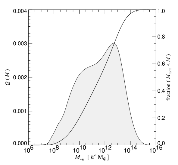
Figure 15: Distribution of the integrated star formation history with respect to halo mass (shaded). This function is the time integral of the multiplicity function of star formation and shows which mass scales are the dominant formation sites of stars. Interestingly, the distribution is quite broad, showing that nearly the same mass in stars forms per decade of halo mass in the range $10^{10}-10^{13.5}\,h^{-1}{\rm M}_{\odot}$, with a slight peak at $\sim 10^{12.5}\,h^{-1}{\rm M}_{\odot}$. We also include a plot of the cumulative function of this distribution (right scale). Roughly half of the stars are predicted to have formed in halos less massive than $10^{11.5}\,h^{-1}{\rm M}_{\odot}$.

Fraction	$z$	$T\;[{\rm Gyr}]$
0.1	5.98	12.55
0.2	4.53	12.17
0.3	3.56	11.73
0.4	2.80	11.19
0.5	2.14	10.44
0.6	1.58	9.45
0.7	1.08	8.03
0.8	0.67	6.12
0.9	0.31	3.48

Table 2: Cumulative star formation history as a function of lookback time $T$ and redshift $z$. This data corresponds to the plots shown in Figure 13.

7 Early star formation as possible source for hydrogen reionisation

There are both observational and theoretical indications that at least some of the ionising background at high redshift comes from stars and that it is not all produced by quasars (e.g. Steidel et al., 2001; Haehnelt et al., 2001; Hui et al., 2002). This is a long debate. At low redshift, it seems clear that quasars dominate, while at high redshift, the space density of bright quasars appears to drop so rapidly that it is difficult to see how they could reionise the Universe already by redshift $z\sim 6$. Hence, it has been speculated extensively that hydrogen was mostly reionised by stars, or possibly harder sources like weak AGN or mini-quasars. Recently, the first determinations of the spectrum of Lyman-break galaxies at redshifts $\left<z\right>=3.4$ by Steidel et al. (2001) have revealed a surprisingly high escape fraction for hydrogen ionising photons, supporting scenarios where the star forming galaxies reionise hydrogen around redshift $z\sim 6$, with quasi-stellar sources taking over only at redshifts $z<3$ (Haehnelt et al., 2001). This general picture is consistent with the analysis of Sokasian et al. (2002b) who have constrained the spectral shape of the UV background at $z\sim 2.5-5$ from the opacities of the HI and HeII Lyman-alpha forests, at an epoch when HeII reionisation is likely to have occurred (Sokasian et al., 2002a).

Here, we roughly estimate whether the star formation rates predicted at high redshift in our model could be responsible for the reionisation of hydrogen by redshift $z\sim 6$. The fact that we infer a star formation rate that peaks around this redshift is certainly intriguing, although this may just be a coincidence.

Figure 16: Clumping factor of the gas in the simulations of the Z-Series as a function of redshift. We show results for Z1, Z2, Z3, and Z4. The clumping factor was estimated for all the gas by means of equation (20).

The reionisation of the universe can be described in a statistical sense by noting that every ionising photon that is emitted is either absorbed by a newly ionised hydrogen atom, or by a recombining one (Madau, 2000). The filling factor $Q(t)$ of regions of ionised hydrogen is then simply given by the total number of ionising photons emitted per hydrogen atom at earlier times than $t$, minus the total number of recombinations per atom. Based on this argument, Madau et al. (1999) derived a simple differential equation that governs the transition from a neutral universe to a fully ionised one:

$$\frac{{\rm d}Q}{{\rm d}t}=\frac{\dot{n}_{\rm ion}}{{\overline{n}_{\rm H}}}-\frac{Q(t)}{\overline{t}_{\rm rec}}.$$ (16)

Here $\dot{n}_{\rm ion}$ is the comoving emission rate of hydrogen ionising photons, ${\overline{n}_{\rm H}}$ is the average comoving density of hydrogen atoms, and $\overline{t}_{\rm rec}$ is the volume averaged hydrogen recombination time. The latter can be expressed as:

$$\overline{t}_{\rm rec}=\frac{1}{(1+z)^{3}(1+2\chi)\,{\overline{n}_{\rm H}}\,\alpha_{B}\,C},$$ (17)

where

$$C\equiv\frac{\left<n_{\rm H^{+}}^{2}\right>}{\left<n_{\rm H^{+}}\right>^{2}}$$ (18)

is the clumping factor of ionised hydrogen, $\chi$ is the helium to hydrogen abundance ratio, and $\alpha_{B}$ is the recombination coefficient. Assuming a gas temperature of $10^{4}\,{\rm K}$, the recombination time can be written as (Madau et al., 1999):

$$\overline{t}_{\rm rec}=588\frac{a^{3}}{C(a)}\,{\rm Gyr}.$$ (19)

We will approximate $C$ with the clumping factor of all the gas, measured directly from the simulations. This will tend to overestimate the clumping slightly, since higher density regions will typically tend to be less ionised. On the other hand, measurements from the simulations are expected to be biased low due to their intrinsic resolution limit.

Figure 17: Filling factor of ionised hydrogen as a function of redshift when the star-forming galaxies are assumed to be the only ionising sources. Results are shown for the different escape fractions of 10%, 50%, and 100%. Interestingly, the star formation history at high redshift might be sufficient to ionise hydrogen even without the proposed population III generation of stars, but only for high escape fractions close to unity.

For the Lagrangian SPH simulations, we can estimate the clumping factor conveniently from

$$C=\frac{\sum_{i}m_{i}\rho_{i}^{-1}\sum_{j}m_{j}\rho_{j}}{\left(\sum_{k}m_{k}\right)^{2}}.$$ (20)

In Figure 16, we show the clumping factors measured in this way for the four simulations Z1-Z4. As expected, for higher mass resolution, there is a tendency to detect an earlier increase of the clumping due to the first structures that form, but overall there is gratifying agreement between the simulations, especially in the most interesting redshift regime of $z\simeq 6-10$. Note that our measured clumping values are also in good agreement with the semi-analytic prediction of Benson et al. (2001).

Madau et al. (1999) estimate that approximately $10^{53}$ ionising photons per second are released by every star forming region with a star formation rate of $1\,{\rm M}_{\odot}\,{\rm yr}^{-1}$. A large uncertainty is to what extent these photons are able to escape a galaxy without being absorbed in the star-forming ISM itself. The escape fraction $f_{\rm esc}$ has been estimated to be quite small at low redshift (e.g. Leitherer et al., 1995), but recent results by Steidel et al. (2001) suggest that it may actually have been quite high in Lyman-break galaxies at high redshift. If these results are confirmed, it could well be above 50% at these redshifts. We model the emission rate as

$$\dot{n}_{\rm ion}=f_{\rm esc}\,\eta\,\dot{\rho}_{\star},$$ (21)

where $\eta=10^{53}\,{\rm phot\;s^{-1}\,M_{\odot}^{-1}yr}$.

For a given value of the escape fraction, the measured evolution of the star formation history and of the clumping factor in the simulations can be used to integrate equation (16) in time. In Figure 17, we show our results for escape fractions of 10%, 50%, and 100%. It is rather interesting to note that for the latter case, we obtain a reionisation redshift of $z\simeq 8$. However, this result is quite sensitive to the assumed escape fraction. Lowering the number of available photons by a factor of 2 will already delay the reionisation redshift to $z\simeq 4$, while an escape fraction as low as 10% together with the strong clumping that develops at low redshift will prevent hydrogen ionisation by stars altogether. By the same token, the result is sensitive to the assumed IMF because the latter influences the production rate of ionising photons. For a Salpeter IMF, Hui et al. (2002) actually estimate $\eta=1.5\times 10^{53}\,{\rm phot\;s^{-1}\,M_{\odot}^{-1}yr}$, which is 50% higher than the value we adopted in our estimate and would thus give more room for lower escape fractions.

It thus appears that hydrogen reionisation by stars at redshifts around $z\sim 6$ is plausible with a cosmic star formation history as predicted here. It requires, however, a high escape fraction. Further observational determinations of the escape fractions, and theoretical studies of radiative transfer in the star forming regions, are clearly needed to shine more light on this important issue. In particular, a quantitative estimate of the escape fraction in a galaxy experiencing a strong wind is desirable, as the sweeping of gas in galaxy halos by these winds should enable high energy photons to escape more easily. Promising attempts to include self-consistent treatments of radiative transfer directly in simulations have already been made (e.g. Gnedin & Ostriker, 1997; Ciardi et al., 2001, 2002; Sokasian et al., 2001), and the recent progress in developing better algorithmic treatments of radiative transfer (e.g. Gnedin & Abel, 2001; Abel & Wandelt, 2002; Cen, 2002) will soon improve the reliability of these computations.

8 Discussion

We have studied the star formation history of the Universe using cosmological SPH simulations that employ a sophisticated treatment of star formation, supernova feedback, and galactic outflows. Using present day computational capabilities, we have been able to show that this model yields numerically converged results for halos of all relevant mass scales, assuming that the vast majority of stars can form only in halos in which gas can condense by atomic line cooling. Using a large set of high-resolution simulations on interlocking scales and at interlocking redshifts, we have been able to determine the multiplicity function of cosmic star formation and infer its evolution from high redshift to the present. We think that the numerical methodology used here represents perhaps the most comprehensive attempt thus far to constrain the cosmic star formation history in the $\Lambda$CDM cosmogony with simulations.

Interestingly, our predicted star formation density peaks early, already at redshifts around $z\sim 5-6$, and then falls to the present time by a factor of about 10. The decline at low redshift is hence shallower than suggested by a subset of observational results, and our star formation rate also appears low at redshifts around $z\sim 1$ compared to some of the data. However, there is very large scatter between different observations, which are partly inconsistent with each other, emphasising the challenges posed by these measurements. Our result matches a number of the observational points, and does so particularly well at very low and very high redshift. We thus conclude that at present our results are consistent with direct data on the star formation rate density as a function of epoch. It will be very interesting to see whether this will remain true when observational uncertainty is reduced in the future.

One consequence of the star formation history we predict is that the majority of stars at the present should be quite old, despite the hierarchical formation of galaxies. Already 10.4 Gyr ago, by redshift $z=2.14$, half of the stars should have formed, with only $\sim 25\%$ forming at redshifts below unity. The mean stellar age at $z=0$ predicted by our model is 9 Gyr.

Integrated over cosmic time, star formation occurs predominantly in halos with masses between $10^{8}\,h^{-1}{\rm M}_{\odot}$ and $10^{14}\,h^{-1}{\rm M}_{\odot}$, with 50% forming in halos below $10^{11.5}\,h^{-1}{\rm M}_{\odot}$. It is thus clear that simulations of galaxy formation need to be able to resolve at least these mass scales well in order to have a chance at giving a reasonably accurate accounting of the formation of the luminous component of the Universe.

The total integrated star formation rate predicts a density in stars of about $\Omega_{\star}=0.004$, or expressed differently, 10% of all baryons should have been turned into long-lived stars by the present. This is in comfortable agreement with recent determinations of the luminosity density of the Universe, while earlier theoretical work was typically predicting substantially larger numbers of stars, by up to a factor of three or so. Our model hence appears to have resolved the so-called “over-cooling crisis”. This was primarily made possible by the strong feedback we adopted in our simulations in the form of galactic winds.

We note that our predictions do depend on the model for star formation and feedback we adopted. In particular, without the inclusion of galactic outflows, which have been introduced on a phenomenological basis in our approach, star formation in the low redshift universe would clearly have been higher. Our strategy has been to normalise the free parameters in our star formation law (the consumption timescale of cold gas) to observations of local disk galaxies, and to select the parameters for the galactic winds as suggested by observations. Under the assumption that the same laws hold roughly at all redshifts, we have then computed what simulations predict for the $\Lambda$CDM model. In this context, one should clearly distinguish between the computational difficulty of the problem on one hand, and the uncertainty and complexity of the modeling of the physics on the other. We think that we have been able to make great progress on the computational side of the problem, but we are aware that large uncertainties remain in our handling of star formation and feedback. It is possible that the modeling of the physics we adopted could be incomplete in crucial respects.

Perhaps one of the most important effects that has been neglected in our simulations is metal line cooling. It is well known that metals can substantially boost cooling rates, and hence can potentially have a very prominent effect on the rates at which gas becomes available for star formation (White & Frenk, 1991). However, the extent to which metal enrichment can enhance gas cooling is strongly dependent on how efficiently metals can be dispersed and mixed into gas that has yet to cool for the first time. In simulations without galactic winds, we find that metals are largely confined to the star-forming ISM at high overdensity. Metal-line cooling would not significantly increase the star formation rates in these simulations. In the present set of simulations, metals can be transported by winds into the low-density IGM. If the corresponding gas is reaccreted at later times into larger systems, metal-line cooling should then accelerate cooling, thereby potentially increasing the total star formation density compared to what we estimated here, particularly at low redshift. But recall that metal line cooling has also been neglected when we normalised the star formation timescale used in our model for the ISM to match the Kennicutt law. If we had included metal line cooling, this normalisation would have been somewhat different in order to compensate for the accelerated cooling, such that the net star formation rate would have again matched the Kennicutt law. This effect will alleviate any difference that one naively expects from the inclusion of metal line cooling. More work is therefore needed to quantitatively estimate how important the effect of metal line cooling would ultimately be in the present model of feedback due to galactic winds.

The set of simulations we carried out offers rich information on many aspects of galaxy formation and structure formation, not only on the cosmic star formation history. Note in particular that our simulations are among the first that can self-consistently address the interaction of winds with the low-density IGM, and the transport of heavy metals along with them. We have already investigated effects of the winds on secondary anisotropies of the cosmic microwave background (White et al., 2002). Among the issues we plan to address next, is the question of whether winds imprint specific signatures in the Lyman-$\alpha$ forest that can be identified observationally..

References

- Abel et al. (2002) Abel T., Bryan G. L., Norman M. L., 2002, Science, 295, 93
- Abel & Wandelt (2002) Abel T., Wandelt B. D., 2002, MNRAS, 330, 53
- Ascasibar et al. (2002) Ascasibar Y., Yepes G., Gottlöber S., Müller V., 2002, A&A, 387, 396
- Baldry et al. (2002) Baldry I. K., Glazebrook K., Baugh C. M., et al., 2002, ApJ, 569, 582
- Balogh et al. (2001) Balogh M. L., Pearce F. R., Bower R. G., Kay S. T., 2001, MNRAS, 326, 1228
- Barkana & Loeb (2000) Barkana R., Loeb A., 2000, ApJ, 539, 20
- Baugh et al. (1998) Baugh C. M., Cole S., Frenk C. S., Lacey C. S., 1998, ApJ, 498, 504
- Benson et al. (2002a) Benson A. J., Lacey C. G., abd S. Cole C. M. B., Frenk C. S., 2002a, MNRAS, 333, 156
- Benson et al. (2002b) Benson A. J., Lacey C. G., abd S. Cole C. M. B., Frenk C. S., 2002b, MNRAS, 333, 177
- Benson et al. (2001) Benson A. J., Nusser A., Sugiyama N., Lacey C. G., 2001, MNRAS, 320, 153
- Bland-Hawthorn (1995) Bland-Hawthorn J., 1995, Proc. Astron. Soc. Australia, 12, 190
- Blanton et al. (1999) Blanton M., Cen R., Ostriker J. P., Strauss M., 1999, ApJ, 522, 590
- Bromm et al. (1999) Bromm V., Coppi P. S., Larson R. B., 1999, ApJ, 527, 5
- Bullock et al. (2000) Bullock J. S., Kravtsov A. V., Weinberg D. H., 2000, ApJ, 539, 517
- Bullock et al. (2001) Bullock J. S., Kravtsov A. V., Weinberg D. H., 2001, ApJ, 548, 33
- Carr et al. (1984) Carr B. J., Bond J. R., Arnett W. D., 1984, ApJ, 277, 445
- Cen (2002) Cen R., 2002, ApJS, 141, 211
- Cen et al. (1994) Cen R., Miralda-Escudé J., Ostriker J. P., Rauch M. J., 1994, ApJ, 437, L9
- Cen & Ostriker (1993) Cen R., Ostriker J. P., 1993, ApJ, 417, 415
- Cen & Ostriker (1999) Cen R., Ostriker J. P., 1999, ApJ, 519, L109
- Cen & Ostriker (2000) Cen R., Ostriker J. P., 2000, ApJ, 538, 83
- Ciardi et al. (2002) Ciardi B., Bianchi S., Ferrara A., 2002, MNRAS, 331, 463
- Ciardi et al. (2001) Ciardi B., Ferrara A., Marri S., Raimondo G., 2001, MNRAS, 324, 381
- Cole (1991) Cole S., 1991, ApJ, 367, 45
- Cole et al. (1994) Cole S., Aragon-Salamanca A., Frenk C. S., Navarro J. F., Zepf S. E., 1994, MNRAS, 271, 781
- Cole et al. (2001) Cole S., Norberg P., Baugh C. M., et al., 2001, MNRAS, 326, 255
- Connolly et al. (1997) Connolly A. J., Szalay A. S., Dickinson M., Subbarao M. U., Brunner R. J., 1997, ApJ, 486, L11
- Cowie et al. (1999) Cowie L. L., Songaila A., Barger A. J., 1999, ApJ, 118, 603
- Cowie et al. (1996) Cowie L. L., Songaila A., Hu E. M., Cohen J. G., 1996, AJ, 112, 839
- Croft et al. (2001) Croft R. A. C., Di Matteo T., Davé R., et al., 2001, ApJ, 557, 67
- Dahlem et al. (1997) Dahlem M., Petr M. G., Lehnert M. D., Heckman T. M., Ehle M., 1997, A&A, 320, 731
- Davé et al. (2001) Davé R., Cen R., Ostriker J. P., et al., 2001, ApJ, 552, 473
- Davé et al. (1999) Davé R., Hernquist L., Katz N., Weinberg D. H., 1999, ApJ, 511, 521
- Flores et al. (1999) Flores H., Hammer F., Thuan T. X., et al., 1999, ApJ, 517, 148
- Frye et al. (2002) Frye B., Broadhurst T., Benitez N., 2002, ApJ, 568, 558
- Fukugita et al. (1998) Fukugita M., Hogan C. J., Peebles P. J. E., 1998, ApJ, 503, 518
- Gallego et al. (1995) Gallego J., Zamorano J., Aragon-Salamanca A., Rego M., 1995, ApJ, 455, L1
- Gnedin & Ostriker (1997) Gnedin N., Ostriker J., 1997, ApJ, 486, 581
- Gnedin & Abel (2001) Gnedin N. Y., Abel T., 2001, New Astronomy, 6, 437
- Gronwall (1999) Gronwall C., 1999, in After the Dark Ages: When galaxies where young, edited by S. Holt, E. Smith, 335, Am. Inst. Phys. Press, Woodbury, NY
- Haardt & Madau (1996) Haardt F., Madau P., 1996, ApJ, 461, 20
- Haehnelt et al. (2001) Haehnelt M. G., Madau P., Kudritzki R., Haardt F., 2001, ApJ, 549, L151
- Heckman et al. (1995) Heckman T. M., Dahlem M., Lehnert M. D., Fabbiano G., Gilmore D., Waller W. H., 1995, ApJ, 448, 98
- Heckman et al. (2000) Heckman T. M., Lehnert M. D., Strickland D. K., Armus L., 2000, ApJS, 129, 493
- Hernquist et al. (1996) Hernquist L., Katz N., Weinberg D. H., Miralda-Escudé J., 1996, ApJ, 457, L51
- Hernquist & Springel (2002) Hernquist L., Springel V., 2002, preprint, astro-ph/0209183
- Hogg (2001) Hogg D. W., 2001, preprint, astro-ph/0105280
- Hughes et al. (1998) Hughes D. H., Serjeant S., Dunlop J., et al., 1998, Nature, 394, 241
- Hui et al. (2002) Hui L., Haiman Z., Zaldarriaga M., Alexander T., 2002, ApJ, 564, 525
- Jang-Condell & Hernquist (2001) Jang-Condell H., Hernquist L., 2001, ApJ, 548, 68
- Jenkins et al. (2001) Jenkins A., Frenk C. S., White S. D. M., et al., 2001, MNRAS, 321, 372
- Katz et al. (1999) Katz N., Hernquist L., Weinberg D. H., 1999, ApJ, 523, 463
- Katz et al. (1996) Katz N., Weinberg D. H., Hernquist L., 1996, ApJS, 105, 19
- Kauffmann et al. (1994) Kauffmann G., Guiderdoni B., White S. D. M., 1994, MNRAS, 267, 981
- Kauffmann et al. (1993) Kauffmann G., White S. D. M., Guiderdoni B., 1993, MNRAS, 264, 201
- Kennicutt (1989) Kennicutt R. C., 1989, ApJ, 344, 685
- Kennicutt (1998) Kennicutt R. C., 1998, ApJ, 498, 541
- Keshet et al. (2002) Keshet U., Waxman E., Loeb A., Springel V., Hernquist L., 2002, preprint, astro-ph/0202318
- Lacey et al. (1993) Lacey C., Guiderdoni B., Rocca-Vomerange B., Silk J., 1993, ApJ, 402, 15
- Lacey & Silk (1991) Lacey C., Silk J., 1991, ApJ, 381, 14
- Lanzetta et al. (2002) Lanzetta K. M., Yahata N., Pascarelle S., Chen H., Fernandez-Soto A., 2002, ApJ, 570, 492
- Lehnert & Heckman (1996) Lehnert M. D., Heckman T. M., 1996, ApJ, 462, 651
- Leitherer et al. (1995) Leitherer C., Ferguson H. C., Heckman T. M., Lowenthal J. D., 1995, ApJ, 454, L19
- Lilly et al. (1996) Lilly S. J., Fevre O. L., Hammer F., Crampton D., 1996, ApJ, 460, L1
- Madau (2000) Madau P., 2000, Philos. Trans. R. Soc. London A, 358, 2221
- Madau et al. (1996) Madau P., Ferguson H. C., Dickinson M. E., Giavalisco M., Steidel C. C., Fruchter A., 1996, MNRAS, 283, 1388
- Madau et al. (1999) Madau P., Haardt F., Rees M. J., 1999, ApJ, 514, 648
- Madau et al. (1998) Madau P., Pozzetti L., Dickinson M., 1998, ApJ, 498, 106
- Martin (1999) Martin C. L., 1999, ApJ, 513, 156
- McKee & Ostriker (1977) McKee C. F., Ostriker J. P., 1977, ApJ, 218, 148
- Mo & White (2002) Mo H. J., White S. D. M., 2002, MNRAS, 336, 112
- Nagamine et al. (2000) Nagamine K., Cen R., Ostriker J. P., 2000, ApJ, 541, 25
- Nagamine et al. (2001) Nagamine K., Fukugita M., Cen R., Ostriker J. P., 2001, ApJ, 558, 497
- Navarro et al. (1996) Navarro J. F., Frenk C. S., White S. D. M., 1996, ApJ, 462, 563
- Navarro et al. (1997) Navarro J. F., Frenk C. S., White S. D. M., 1997, ApJ, 490, 493
- Pascarelle et al. (1998) Pascarelle S. M., Lanzetta K. M., Fernandez-Soto A., 1998, ApJ, 508, L1
- Pearce et al. (1999) Pearce F. R., Jenkins A., Frenk C. S., et al., 1999, ApJ, 521, L99
- Pearce et al. (2001) Pearce F. R., Jenkins A., Frenk C. S., et al., 2001, MNRAS, 326, 649
- Pettini et al. (2001) Pettini M., Shapley A. E., Steidel C. C., et al., 2001, ApJ, 554, 981
- Pettini et al. (2000) Pettini M., Steidel C. C., Adelberger K. L., Dickinson M., Giavalisco M., 2000, ApJ, 528, 96
- Press & Schechter (1974) Press W. H., Schechter P., 1974, ApJ, 187, 425
- Scannapieco et al. (2001) Scannapieco E., Thacker R. J., Davis M., 2001, ApJ, 557, 605
- Sheth et al. (2001) Sheth R. K., Mo H. J., Tormen G., 2001, MNRAS, 323, 1
- Sheth & Tormen (1999) Sheth R. K., Tormen G., 1999, MNRAS, 308, 119
- Sheth & Tormen (2002) Sheth R. K., Tormen G., 2002, MNRAS, 329, 61
- Sokasian et al. (2002a) Sokasian A., Abel T., Hernquist L., 2002a, MNRAS, 332, 601
- Sokasian et al. (2002b) Sokasian A., Abel T., Hernquist L., 2002b, preprint, astro-ph/0206428
- Sokasian et al. (2001) Sokasian A., Abel T., Hernquist L. E., 2001, New Astronomy, 6, 359
- Somerville (2002) Somerville R. S., 2002, ApJ, 572, 23
- Somerville et al. (2001) Somerville R. S., Primack J. R., Faber S. M., 2001, MNRAS, 320, 504
- Springel & Hernquist (2002a) Springel V., Hernquist L., 2002a, preprint, astro-ph/0206393
- Springel & Hernquist (2002b) Springel V., Hernquist L., 2002b, MNRAS, 333, 649
- Springel et al. (2001) Springel V., Yoshida N., White S. D. M., 2001, New Astronomy, 6, 79
- Steidel et al. (1999) Steidel C. C., Adelberger K. L., Giavalisco M., Dickinson M., Pettini M., 1999, ApJ, 519, 1
- Steidel et al. (2001) Steidel C. C., Pettini M., Adelberger K. L., 2001, ApJ, 546, 665
- Steinmetz & Müller (1995) Steinmetz M., Müller E., 1995, MNRAS, 276, 549
- Thacker & Couchman (2000) Thacker R. J., Couchman H. M. P., 2000, ApJ, 545, 728
- Thacker et al. (2000) Thacker R. J., Tittley E. R., Pearce F. R., Couchman H. M. P., Thomas P. A., 2000, MNRAS, 319, 619
- Tresse & Maddox (1998) Tresse L., Maddox S. J., 1998, ApJ, 495, 691
- Treyer et al. (1998) Treyer M. A., Ellis R. S., Milliard B., Donas J., Bridges T. J., 1998, MNRAS, 300, 303
- Weinberg et al. (1999) Weinberg D. H., Davé R., Gardner J. P., Hernquist L., Katz N., 1999, in Photometric Redshifts and the Detection of High Redshift Galaxies, edited by R. Weymann, L. Storrie-Lombardi, M. Sawicki, R. Brunner, vol. 191, ASP Conference Series, 341
- Weinberg et al. (1997) Weinberg D. H., Hernquist L., Katz N., 1997, ApJ, 477, 8
- Weinberg et al. (2002) Weinberg D. H., Hernquist L., Katz N., 2002, ApJ, 571, 15
- White et al. (2002) White M., Hernquist L., Springel V., 2002, preprint, astro-ph/0205437
- White & Frenk (1991) White S. D. M., Frenk C. S., 1991, ApJ, 379, 52
- White & Rees (1978) White S. D. M., Rees M. J., 1978, MNRAS, 183, 341
- Wilson et al. (2002) Wilson G., Cowie L. L., Barger A. J., Burke D. J., 2002, AJ, 124, 1258
- Yepes et al. (1997) Yepes G., Kates R., Khokhlov A., Klypin A., 1997, MNRAS, 284, 235
- Yoshida et al. (2002) Yoshida N., Stöhr F., Springel V., White S. D. M., 2002, MNRAS, 335, 762
- Zhang et al. (1995) Zhang Y., Anninos P., Norman M. L., 1995, ApJ, 453, L57