Stability and heating of magnetically driven jets from Keplerian accretion discs

Abstract

We have performed 3-D numerical magnetohydrodynamic (MHD) jet experiments to study the instabilities associated with strongly toroidal magnetic fields. In contemporary jet theories, a highly wound up magnetic field is a crucial ingredient for collimation of the flow. If such magnetic configurations are as unstable as found in the laboratory and by analytical estimates, our understanding of MHD jet driving and collimation has to be revised.

A perfectly conducting Keplerian disc with fixed density, rotational velocity and pressure is used as a lower boundary for the jet. Initially, the corona above the disc is at rest, permeated by a uniform magnetic field, and is in hydrostatic equilibrium in a softened gravitational field from a point mass. The mass ejection from the disc is subsequently allowed to evolve according to deviations from the initial pressure equilibrium between disc and corona.

The energy equation is solved, with the inclusion of self-consistently computed heating by viscous and magnetic dissipation. We find that magnetic dissipation may have profound effects on the jet flow as: 1) it turns on in highly wound up magnetic field regions and helps to prevent critical kink situations; 2) it influences jet dynamics by re-organizing the magnetic field structure and increasing thermal pressure in the jet; and 3) it influences mass loading by increasing temperature and pressure at the base of the jet.

The resulting jets evolve into time-dependent, non-axisymmetric configurations, but we find only minor disruption of the jets by e.g. the kink instability.

1 Introduction

Though astrophysical jets have been observed in a rather wide range of accreting systems, it is generally assumed that the mechanism for acceleration and collimation is generic (Livio, 1997; Spruit, 2000, for recent reviews). Contemporary jet theories rely on magnetic forces as the jet producing mechanism, either with the flow emanating from the disc surface and associated with an open magnetic field structure Blandford and Payne (1982) or with the flow emanating from the disc-star interface and associated with a closed field structure connecting disc and central star Pringle (1989). In the former so-called disc-wind scenario, which is currently receiving most attention, the driving force, acting to overcome the gravitational pull of the central object, is typically regarded as a component of the centrifugal force along the magnetic field. However, adopting an inertial frame of reference the driving mechanism may equally be interpreted as magnetic Spruit (1996). The inertia of the outflowing gas eventually becomes dynamically important and the gas stops corotating with the underlying disc. At this point the magnetic field, which cannot easily slip through the highly ionized gas, is wound up in a cork screw manner between the disc and the vertically accelerated and less quickly rotating outflow. The tension (“hoop stress”) of the wound-up magnetic field configuration is generally believed to be the collimating force, but collimation by a poloidal field has been proposed as well Spruit et al. (1997) motivated by instability arguments against the wound-up field scenario.

The assumed large scale magnetic field in the disc-wind scenario may either be provided by dynamo processes in the disc Brandenburg (2000); Bardou et al. (2001) or captured from the environment and advected inwards by the accreting matter Cao and Spruit (1994). Numerical work has been carried out to investigate situations in which a significant fraction of the field lines loop back into the disc Romanova et al. (1998); Turner et al. (1999). These experiments have focused on the ejection and acceleration mechanisms as well as the evolution of the magnetosphere close to the disc, and have not followed the flow further out for extended times.

The numerical work done in relation to the “classical” large scale open field scenario may be divided into experiments attempting to include (parts of) the accretion disc in the computational domain Uchida and Shibata (1985); Bell and Lucek (1995) and more recent work Ustyugova et al. (1995); Ouyed et al. (1997); Meier et al. (1997) which has used the disc only as a fixed lower boundary to avoid problems with radial collapse of the disc and thereby relatively short time evolution of the experiment. Both types of experiments have been axisymmetric and as such have not questioned the potentially (kink) unstable wound up magnetic field configuration on which the collimation process relies. However, Spruit et al. Spruit et al. (2001) have recently proposed fast reconnection processes in more disordered non-axisymmetric large scale magnetic fields in the jet like gamma ray burst (GRB) scenario. The magnetic dissipation is proposed for the GRB fireballs e.g. to produce the observed radiation with better efficiency. We find that such magnetic processes may have severe impact on jet dynamics and stability in particular.

The main purpose of the work presented here is to establish whether or not the jets in the disc-wind scenario are prone to catastrophic MHD instabilities. This calls for an implementation of a setup in three dimensions which will be described in Sect. 2. For simplicity, we assume a large-scale open magnetic field structure and use the disc as a fixed boundary. The details of the initial conditions and boundary conditions are found in Sect. 2.2 and 2.3 respectively. Results are presented in Sect. 3, with Sect. 3.1 concentrating on the jet dynamics and Sect. 3.2 on the observed 3-D jet stability in the experiments. In Sect. 4 we discuss the results with special emphasis on thermal properties and magnetic field structure. Finally, the paper is summarized and conclusions are presented in Sect. 5.

2 Model

The jet flow is described numerically by solving the MHD equations in the following form;

$$\frac{\partial\rho}{\partial t}=-\nabla\cdot\rho\mathbf{u},$$ (1)

$$\frac{\partial(\rho\mathbf{u})}{\partial t}=-\nabla\cdot\left(\rho\mathbf{uu}-\tau^{\prime}\right)+\nabla P+\mathbf{J\times B}-\rho\nabla\Phi,$$ (2)

$$\mu\mathbf{J}=\nabla\times\mathbf{B},$$ (3)

$$\mathbf{E}=\eta\mathbf{J}-\mathbf{u\times B},$$ (4)

$$\frac{\partial\mathbf{B}}{\partial t}=-\nabla\times\mathbf{E},$$ (5)

$$\frac{\partial e}{\partial t}=-\nabla\cdot e\mathbf{u}-P\nabla\cdot\mathbf{u}+Q,$$ (6)

where $\rho$ is the mass density, $\mathbf{u}$ the velocity vector, $\tau^{\prime}$ the viscous stress tensor, $P$ the thermal gas pressure, $\Phi$ the gravitational potential, $\mathbf{B}$ the magnetic flux density vector, $\mathbf{J}$ the electric current density vector, $\mathbf{E}$ the intensity of the electric field, $\eta$ the electric resistivity, $e$ the internal energy per unit volume and $Q$ the sum of viscous and Joule dissipation.

2.1 Dimensions and numerics

Quantity	Unit	YSO	AGN
Velocity	$\sqrt{GM/\lambda}$	$138\,\mathrm{km/s}$	$0.2\,c$
Time	$\sqrt{\lambda^{3}/(GM)}$	$0.58\,\mathrm{days}$	$0.51\,\mathrm{days}$
Mass density	$\mathcal{B}^{2}\lambda/(\mu_{0}GM)$	$4.2\times 10^{-14}\,\mathrm{g/cm^{3}}$	$1.8\times 10^{-17}\,\mathrm{g/cm^{3}}$

Table 1: The magnetic permeability is denoted by $\mu_{0}$. Representative values are listed for a young stellar object (YSO) with $M=1\,M_{\sun}$, $\mathcal{B}=10\,\mathrm{G}$, and $\lambda=10\,R_{\sun}$. Likewise, an entry is included for a typical active galactic nucleus (AGN) of $M=10^{8}\,M_{\sun}$, $\mathcal{B}=100\,\mathrm{G}$ and $\lambda=10\,R_{\mathrm{S}}$, where the Schwarzschild radius is given by $R_{\mathrm{S}}=2GM/c^{2}$.

Both for numerical reasons and to be able to adapt the calculations to stellar as well as galactic scales, the physical quantities are given in units of characteristic quantities of the system. The form of the equations are not changed by converting to this system of units. The appropriate units may be constructed from the mass of the central object, $M$, the magnetic flux density, $\mathcal{B}$, and the length scale, $\lambda$. The characteristic length scale $\lambda$ is assumed to correspond to the inner disc radius. If not otherwise stated, the dimensionless quantities listed in Table 1 are used in the following sections.

The code uses a sixth order accurate method for partial derivatives and a fifth order accurate interpolation method with the variables represented in non-uniform (Eulerian) staggered meshes Nordlund and Galsgaard (1997a); Rögnvaldsson (1999). In the discrete representation of quantities, the scalar variables ($e$ and $\rho$) are zone centered and components of the vector variables ($\mathbf{p}=\rho\mathbf{u}$ and $\mathbf{B}$) are face centered in a unit mesh volume. The solution for the eight variables, $\rho$, $e$, $p_{x}$, $p_{y}$, $p_{z}$, $B_{x}$, $B_{y}$, $B_{z}$ is advanced in time by a third order predictor-corrector procedure Hyman (1979), modified to accommodate variable time steps. The code has previously been verified by a number of standard test problems and henceforth been used for experiments involving 3-D turbulence Nordlund et al. (1994), investigations of problems related to coronal heating Nordlund and Galsgaard (1997b), buoyant rise of magnetic flux tubes Dorch and Nordlund (1998), dynamo experiments Dorch et al. (1999), stellar convection Nordlund and Stein (2000) and magnetized cooling flows Rögnvaldsson et al. (2002).

Cartesian coordinates ($x,y,z,$) are used to describe the disc-corona system in the computational box. To calculate the derivative or the interpolated value at a given point, the six nearest grid points are involved. As exactly the same operators are used in the whole grid, three layers of ghost zones must be added to prevent periodic wrapping of the computational domain. For (obsolete) reasons of computational efficiency, we use $x$ (first index) as the vertical direction and place ghost zones in the index range $i\in[1:3]\wedge[m_{x}-3:m_{x}]$. The $y$- and $z$-directions are taken to be periodic. The ($y,z$) cross section of the computational domain is quadratic, both in terms of number of grid points ($m_{y}=m_{z}$) and physical size ($L_{y}=L_{z}$), and centered so that $y\in[-L_{y}/2,L_{y}/2]$ and $z\in[-L_{z}/2,L_{z}/2]$. Only odd numbers of $m_{y}$ and $m_{z}$ have been chosen, making $(x,y,z)=(0,0,0)$ at zone center $(i,j,k)=(4,(m_{y}+1)/2,(m_{z}+1)/2)$.

2.2 Initial conditions

To investigate the magnetic driving and collimation of outflows it is desirable to choose an initial state in which all other dynamical effects are small. Therefore, to obtain such a state, the corona is assumed at rest and in hydrostatic equilibrium in the gravitational field of a point mass Ouyed and Pudritz (1997). Self-gravity of the gas is neglected. A current free configuration is chosen so that the Lorentz force vanishes. In this way, the momentum equation for the corona reduces to

$$\nabla P=-\rho\nabla\Phi.$$ (7)

By the use of a polytropic equation of state, $P=K\rho^{\gamma}$, the reduced momentum equation may be integrated, giving the density distribution for the corona,

$$\rho=\left[(\Phi_{0}-\Phi)\frac{\gamma-1}{K\gamma}\right]^{\frac{1}{\gamma-1}},\quad\gamma\neq 1.$$ (8)

A positive value of the integration constant, $\Phi_{0}\geq 0$, may be introduced to keep finite densities at large distances. The value of the polytropic exponent is chosen to be $\gamma=5/3$, corresponding to an adiabatic mono-atomic ideal gas.

For numerical reasons, the gravitational potential is smoothed by introducing a so-called softening parameter, $l_{\mathrm{s}}$,

$$\Phi=-\frac{1}{\sqrt{x^{2}+y^{2}+z^{2}+l_{\mathrm{s}}^{2}}}.$$ (9)

Due to the location of the gravitational potential in the staggered meshes, a non-zero softening parameter is necessary to make the potential well-defined at $x=y=z=0$. Furthermore, a softened potential makes the potential gradient and the initial density gradient less steep close to the central object and therefore easier to handle by the numerical code. The softening parameter was chosen to be $l_{\mathrm{s}}=\sqrt{1/2}$, for the experiments actually reported herein.

The disc surface (lower boundary) is assumed to have a density distribution described by Eq. 8, and the corona is in pressure balance with the underlying disc. In the case of negligible thermal pressure, the softened potential gives rise to an equilibrium Keplerian like velocity structure in the disc given by

$$u_{y} = \frac{z}{(y^{2}+z^{2}+l_{\mathrm{s}}^{2})^{3/4}},$$

$$u_{z} = -\frac{y}{(y^{2}+z^{2}+l_{\mathrm{s}}^{2})^{3/4}}.$$ (10)

Numerical experiments relying on a smoothed or softened potential produce generally weaker jets Bell and Lucek (1995). Due to the reduced rotation velocity obtained when softening is introduced a longer time scale for the build up of the azimuthal field (and the jet flow) is anticipated. Devising identical experiments and only varying softening, we find no significant effect in jet features but only a scaling of dynamical quantities. The main effect of softening is an increase of the rotational period which scales the characteristic time and the specific kinetic energy (cf. Fig. 1).

In the chosen numerical setup, a density jump at the disc-corona interface must be applied with some caution, as the interpolation of the zone centered values could artificially bring mass into the corona. A density jump may however be implemented to have effect on the energy flux as is demonstrated in Sect. 2.3 below. The pressure balance between disc and corona together with the assumed disc density structure expressed by Eq. 8 implies that a density jump may equivalently be regarded as a jump in internal energy per unit mass, $T\sim P/\rho$. Hence, the jump $\xi\equiv(T_{\mathrm{corona}}/T_{\mathrm{disc}})_{0}$ at the disc-corona interface expresses a jump in (isothermal) sound speed as well; $c_{\mathrm{s,disc}}^{2}=c_{\mathrm{s,corona}}^{2}/\xi$. For $c^{2}_{\mathrm{s,disc}}\ll(u^{2}_{y}+u^{2}_{z})$, the radial pressure gradient in the disc, $\partial p/\partial r\sim(\rho c_{\mathrm{s}}^{2})_{\mathrm{disc}}/R$, becomes negligible compared to the centrifugal force and the pressure gradient does not influence the radial balance of the disc. Anyway, since the disc is not simulated, the disc structure will not be of a numerical concern.

A constant vertical magnetic field, $B_{x}=B_{0}$, is chosen to penetrate both disc and corona initially. In a more realistic case, one may expect the field to be inclined with respect to the disc surface and the field strength is likely to increase towards the center due to advection by the accreting matter Cao and Spruit (1994). Because of the periodic boundaries, such a magnetic field configuration would not be divergence free in the present setup. Furthermore, a field configuration facilitating wind ejection is expected to be generated automatically by the rotation of the disc Ouyed and Pudritz (1997). Therefore, only the simple constant vertical magnetic field configuration has been implemented as initial condition.

The magnetic flux density is specified by the parameter $\beta_{\mathrm{i}}\equiv P_{\mathrm{gas,i}}/P_{\mathrm{mag,i}}$, at $r_{\mathrm{i}}=1$. In the numerical experiment, the density distribution is determined from Eq. 8 with $K=(\gamma-1)/\gamma$. Using $P_{\mathrm{gas}}=K\rho^{\gamma}$ and $P_{\mathrm{mag}}=B_{0}^{2}/2$ it follows that

$$B_{0}=\sqrt{\frac{2K}{\beta_{\mathrm{i}}}\left(\Phi_{0}+\frac{1}{\sqrt{1+l_{\mathrm{s}}^{2}}}\right)^{\frac{\gamma}{\gamma-1}}}.$$ (11)

2.3 Boundary conditions

The disc boundary is located in the $x=0$ plane and is assumed to be a fixed base for the jet. As such, the rotational velocity, mass density and internal energy density is kept constant at their initially prescribed values. Jet fluxes of mass, energy and momentum are assumed to have negligible impact on the disc surface layer. For instance, the disc is assumed to supply mass to the surface at the same rate as the jet carries mass away. This is implemented as a steady condition where the mass flux $p_{x}$ is symmetric at the lower boundary. The energy flux at the disc surface has been implemented as either a zero x-derivative condition or a cold condition. The cold condition is applied by assuming a jump in internal energy per unit mass (temperature) between disc and corona. The internal energy density in the disc ghost zones are found by antisymmetrizing the $x$-face centered values of $T\equiv e/\rho$ around $(e_{0}/\rho_{0})/\xi$;

$$T[b-i+1/2]=2(e_{0}/\rho_{0})/\xi-T[b+i-1/2],$$ (12)

with $b=4$ and $i=1,2,3,4$ so that the values in square brackets are the grid locations. The fixed internal energy density and mass density at the disc surface is denoted $e_{0}$ and $\rho_{0}$ respectively. The temperature jump is specified by the ratio $\xi=(T_{\mathrm{corona}}/T_{\mathrm{disc}})_{0}$ evaluated at the disc-corona interface. In effect, a cold inflow condition is specified by the internal energy density flux, $h_{x}\equiv p_{x}T$.

The inflow velocity is not specified, but allowed to evolve freely according to the forces acting on the disc surface. However, the $x$-flux of $x$-momentum (the $xx$-component of the Reynolds stress tensor) is not allowed to change the outflow velocity on the surface. Instead, thermal and magnetic forces are taken to be the dominant mechanisms for injecting gas into the corona. The pressure in the disc (ghost zones) and on the boundary is kept fixed at the values prescribing the initial pressure balance. Any pressure gradient at the disc surface is caused solely by deviations from the initial hydrostatic equilibrium occurring in the corona.

For the evolution of the magnetic field the disc is taken to be perfectly conducting. In general, the magnetic field is only specified initially and is subsequently evolving according to the electric field. Keeping this in mind when imposing boundary conditions, violation of the divergence free condition of the magnetic field may be prevented in a natural way. Particularly, one finds that the disc velocities determine the electric field and thereby the evolution of the magnetic field at the lower boundary. The electric field on the disc surface is specified as

$$E_{y} = -u_{z}B_{0},$$

$$E_{z} = u_{y}B_{0},$$ (13)

where $B_{0}$ is the constant vertical field specified initially by Eq. 11. The issues of boundary driving is discussed further in Sect. 2.3.1.

At the upper boundary, an extrapolation of the electric field would not be stable and another approach has to be applied which is discussed in Sect. 2.3.2. For the mass, momentum and energy density fluxes, a simple extrapolation into the ghost zones may be applied to allow the densities to evolve on the boundary.

2.3.1 Boundary driving

At the lower boundary the disc is kept rotating with a fixed angular velocity. This should in principle be sufficient to determine the evolution of the $y$- and $z$-components of the magnetic field. It turns out, though, that the velocity driving has to be specified in a somewhat non-local manner. This is because of the non-local nature of the numerical differential operators used in the code. The numerical scheme involves the three nearest points on each side along the direction of differentiation. Therefore, to avoid ripples when driving, the driving has to be passed smoothly to the active grid. To be specific, the velocity field just inside the active grid is determined by passing a third order polynomial through the boundary and the two neighboring zones further inside the grid,

$$u_{i}[5]=\frac{4}{9}u_{i}[4]+\frac{6}{9}u_{i}[6]-\frac{1}{9}u_{i}[7],\quad i=y,z,$$ (14)

where the lower boundary is located at zone index 4. The above chosen polynomial representation has been found in other but similar experiments to give the smoothest driving Nordlund and Galsgaard (1997a). It has not been subjected to tests in the present work.

Care has to be taken also to avoid ripples caused by the periodicity of the $y$- and $z$-boundaries and by the shape of the box. To avoid shear at the box sides and reversed vorticity at the box corners, the disc velocity profile has to be terminated inside the periodic boundaries. As above, the non-local nature of the differential operators demands the decrease of disc rotation to span a few grid points. For the same reason, the velocity cutoff has to take place at some distance from the boundaries to ensure a region of practically zero rotation. To satisfy these conditions, a hyperbolic tangent function is used to cut off the velocity;

$$f_{i}(r)=\frac{1}{2}\left[\tanh\left(\frac{L_{i}}{2}-s_{i}-r\right)+1\right],\quad i=y,z.$$ (15)

Here $L_{i}$ is the size of the box in the $i$ direction and $s_{i}$ is the distance that the midpoint of the hyperbolic cutoff is shifted from the boundary. The resulting velocity profile, $u_{i,\mathrm{cut}}=u_{i}f_{i}$, is shown in Fig. 1 for $L_{y}=L_{z}=30$ and $s_{y}=s_{z}=2.5$ in a slice along $y=0$ and $z\geq 0$.

Figure 1: Plots of the rotational velocity in the disc for different values of the softening parameter, $l_{\mathrm{s}}$. The solid, dotted, dashed and long dashed lines represent values of $l_{\mathrm{s}}=0$ (Keplerian), $1/2$, $\sqrt{1/2}$ and 1 respectively. The plotted profile is given by, $u(r)=u_{\theta}f$ where $u_{\theta}=r/(r^{2}+l_{\mathrm{s}}^{2})^{3/4}$. The cutoff function $f$ terminates the rotation at the periodic boundary ($r\gtrsim 10$) but does not affect the inner regions of the disc.

2.3.2 The quasi-transmitting boundary

A symmetric condition on the electric field does not allow tangential components of the magnetic field to evolve on the boundary. In particular, when the initial winding of the vertical magnetic field reaches the upper boundary as a toroidal Alfvén wave, it would be reflected. To minimize reflection (reversal of the toroidal magnetic field) and possible disruptive and/or decelerating effects on the flow, an upstream sensing of changes in the magnetic field is used to guide the evolution of the boundary field. This may appear somewhat artificial, but it corresponds roughly to apply values along an outgoing characteristic of a linear torsional Alfvén wave. Such a wave propagates with the Alfvén speed $u_{\mathrm{A}}=B_{x}/\sqrt{\rho}$. As a fair estimate, changes in the tangential field are taken to propagate with the (fixed) Alfvén speed determined by

$$u_{\mathrm{A},x}=\frac{B_{0}}{\sqrt{(\Phi_{0}-\Phi)^{\frac{1}{\gamma-1}}}},$$ (16)

evaluated at the upper boundary.

The tangential magnetic field on the boundary is assumed to evolve towards some upstream value at a distance $\Delta x_{\mathrm{up}}$, below the boundary. The travel time is estimated from the Alfvén speed; $t_{\mathrm{up}}=\Delta x_{\mathrm{up}}/u_{\mathrm{A},x}$. The condition implemented on the electric field specifies the evolution of the tangential magnetic field as

$$\frac{\partial B_{i}}{\partial t}=\frac{\Delta B_{i,\mathrm{up}}}{t_{\mathrm{up}}},\quad i=y,z.$$ (17)

The work done on the field may be controlled by the parameter $\chi$, which specifies the convergence values for the magnetic field at the upper boundary;

$$\Delta B_{i,\mathrm{up}}=B_{i}[m_{x}-4]-\chi B_{i}[m_{x}-4-n_{x}],\quad i=y,z.$$ (18)

Here, $n_{x}$ specifies the index width of the sensing distance. Choosing $\chi\lesssim 1$ mimics in a simple way the work done on the magnetic field by the part of the jet outside the computational box.

It must be emphasized, that the $\chi$ parameter is to be regarded as a real physical parameter expressing to what extent the exterior is “braking” the field rotation. If, for example, the field is anchored to massive regions in the ambient medium outside the computational domain, the braking will cause the field to become inclined with respect to the outer boundary. Hence, the choice of $\chi$ is not only a question of numerics, but reflects a real physical degree of freedom.

2.4 Note on approach

The model philosophy adopted here is different from previous work, particularly in the applied boundary conditions. Instead of using large efforts on designing (artificially) open outer boundary conditions, periodic boundaries have been applied. The argument being, that it is inconceivable that real jets would not be perturbed by motions in the surrounding medium anyway. In the present work, the outer boundaries as well as numerical noise provide the perturbations triggering the possible instabilities we wish to investigate. Obviously, this approach cannot provide precise determinations of e.g. growth rates, but it is used to allow instabilities to develop in a natural way and provide indications on whether our understanding of jet collimation needs to be revised or not.

3 Results

The numerical experiments all show the same overall evolutionary sequence which may be summarized as follows:

1. Winding and opening of the magnetic field lines.

2. Relaxation of initial magnetic acceleration and spurious magnetic reflections.

3. Build up of collimated (but unsteady) outflow.

Initially, the winding of the magnetic field propagates through the computational box as a torsional Alfvén wave. The winding propagates with velocities expected to vary with distance approximately as Eq. 16. Accordingly the winding propagates faster at large radii as noted also by Ouyed and Pudritz Ouyed and Pudritz (1997).

The upper boundary condition on the magnetic field allows (partially) for the Alfvén pulse to be transmitted. Some reflections are unavoidable, but eventually the reflections are transmitted through the boundaries and the system settles down. The relaxation of the minor Alfvén pulse reflections concludes the two initial phases of the numerical experiments. At which evolutionary stage a (significant) collimated outflow is initiated in a real accreting system can only be speculated upon. In the present type of jet experiment, the initial phases do not reveal much relevant physics and the initial conditions as well as boundary conditions are probably not well suited for such investigations. However, the setup eventually provides a collimated outflow with the expected qualities that we want to investigate.

A set of parameters have been introduced to truncate the physical problem and adopt it into a numerical setup. To probe the effect of these parameters, such as softening, box size and velocity cutoff, a range of experiments were carried out. The truncation of the problem and the effect of the related parameters have been presented above. In what follows, we will concentrate on a small number of experiments which have been conducted particularly to investigate stability issues. These experiments are listed in Table 2.

run	$m_{x}\times m_{y}\times m_{z}$	$L_{x}\times L_{y}\times L_{z}$	$\beta_{\mathrm{i}}$	$\xi$	$t_{\mathrm{max}}$
i	$98\times 71\times 71$	$40\times 30\times 30$	5	1	500
ii	$98\times 71\times 71$	$40\times 30\times 30$	10	1	500
iii	$98\times 71\times 71$	$40\times 30\times 30$	5	100	500
iv	$128\times 85\times 85$	$60\times 40\times 40$	10	1	400
v	$200\times 101\times 101$	$200\times 25\times 25$	10	1	260

Table 2: List of experiments for the stability study. All experiments use the softening parameter, $l_{\mathrm{s}}=\sqrt{1/2}$, and a polytropic index, $\gamma=5/3$.

3.1 Jet dynamics

By examining the rates of change of energies, the action of various forces and issues of stationarity may be analyzed. The rate of change of total energy in a volume of gas is controlled by the rate of energy transport in and out of the volume, i.e. the net flux, $\Delta F=F(x_{\mathrm{lower}})-F(x_{\mathrm{upper}})$, the rate of energy conversion through work, $W$, and dissipation, $Q$. Consequently, the rate of change of magnetic, $\mathcal{M}$, kinetic, $\mathcal{K}$, thermal, $\mathcal{T}$, and gravitational energy, $\mathcal{G}$, in a volume may be expressed as follows,

$$\frac{\partial\mathcal{M}}{\partial t}=\Delta F_{\mathrm{mag}}+W_{\mathrm{Lorentz}}-Q_{\mathrm{Joule}},$$ (19)

$$\frac{\partial\mathcal{K}}{\partial t}=\Delta F_{\mathrm{kin}}+\Delta F_{\mathrm{visc}}+W_{\mathrm{grav}}-W_{\mathrm{gas}}-W_{\mathrm{Lorentz}}-Q_{\mathrm{visc}},$$ (20)

$$\frac{\partial\mathcal{T}}{\partial t}=\Delta F_{\mathrm{enth}}+W_{\mathrm{gas}}+Q_{\mathrm{visc}}+Q_{\mathrm{Joule}},$$ (21)

$$\frac{\partial\mathcal{G}}{\partial t}=\Delta F_{\mathrm{grav}}-W_{\mathrm{grav}}.$$ (22)

The rate of total work done by gravity in the box, $W_{\mathrm{grav}}$, the rate of work done against gas pressure gradients, $W_{\mathrm{gas}}$, and the rate of work done against the Lorentz force, $W_{\mathrm{Lorentz}}$, are given by

$$W_{\mathrm{grav}}=-\int_{V}\mathbf{u}\cdot\rho\nabla\Phi\,dV,$$ (23)

$$W_{\mathrm{gas}}=\int_{V}\mathbf{u}\cdot\nabla P\,dV,$$ (24)

$$W_{\mathrm{Lorentz}}=-\int_{V}\mathbf{u}\cdot\left(\mathbf{J\times B}\right)\,dV.$$ (25)

Here $dV\equiv dx\,dy\,dz$ is an element of the volume, $V=[x_{\mathrm{lower}},x_{\mathrm{upper}}]\times[-L_{y}/2,L_{y}/2]\times[-L_{z}/2,L_{z}/2]$ . The energy fluxes through a cross section, $x$, are given by

$$F_{\mathrm{mag}}(x)=\int_{S}(E_{y}B_{z}-E_{z}B_{y})\,dS_{x},$$ (26)

$$F_{\mathrm{kin}}(x)=\int_{S}u_{x}\left(\frac{1}{2}\rho u^{2}\right)\,dS_{x},$$ (27)

$$F_{\mathrm{enth}}(x)=\int_{S}\rho u_{x}\gamma e\,dS_{x},$$ (28)

$$F_{\mathrm{grav}}(x)=\int_{S}\rho u_{x}\Phi\,dS_{x},$$ (29)

where $dS_{x}\equiv dy\,dz$ represents the element of a surface normal to the $x$-direction and the surface, $S=[-L_{y}/2,L_{y}/2]\times[-L_{z}/2,L_{z}/2]$, is an entire cross section of the box.

Figure 2: Time averaged total energy fluxes as functions of height for run 2 (left panel) and run 2 (right panel). The dotted line is magnetic flux, dashed line is the sum of kinetic and magnetic fluxes, the dot-dashed line is the sum of enthalpy, kinetic and magnetic fluxes. The solid line is the total energy flux, which is obtained by adding the (negative) flux of gravitational energy to the sum of the other fluxes (dot-dashed line).

To demonstrate the quasi-stationary state of the flow and the general energy conversion mechanisms, the time averaged energy fluxes (Eqs. 26–29) are plotted in Fig. 2 as functions of height above the disc. The fluxes are obtained as differences between the curves as indicated by the arrows in the plots.

For both experiments it is seen that more magnetic energy is transported into the volume than is carried out. The magnetic energy does not increase accordingly, since the difference between magnetic energy flux in and out of the volume is balanced on average by Lorentz work and Joule dissipation. The conversion of magnetic energy flux into kinetic energy flux is dominant close to the disc, whereas magnetic energy flux is primarily converted into thermal energy flux in the upper two thirds of the box for both the experiments. Just above the disc surface, a (hydrostatic) balance is seen to be maintained between gravitational energy flux and the sum of enthalpy and kinetic energy flux. This corresponds to a situation where gravity is balanced by gas pressure and $x$-advection of momentum. The two experiments differ significantly in the amount of magnetic energy flux converted into thermal energy flux as a consequence of the difference in the magnetic energy reserve at hand.

Figure 3: The rate of change of magnetic, kinetic and thermal energy in the box between $x=1.1$ and $x=38.8$ are graphed for run 2 (left panels) and run 2 (right panels). The top panels show rate of change of magnetic energy (dotted line), the net Poynting flux into the volume (solid line) and the rate of work done by the Lorentz force (dot-dashed line). The middle panels show rate of change of kinetic energy (dotted line), net kinetic flux into the volume (solid line) and the rate of work against gravity done by carrying matter through the volume (dot-dashed line). The lower panels show rate of change of thermal energy in the volume (dotted line), net enthalpy flux (solid line) and the rate of work done by gas pressure (dot-dashed line). The dashed line marks zero rate of change of energy. Please note that until $t=150$ only 10 snap shots were saved (at time intervals $\Delta t=15$).

Details of the energy conversion processes as a function of time are shown in Fig. 3. After a sharp increase of kinetic energy, caused by the initial Alfvén pulse, the rate of change of kinetic energy oscillates as does the rate of work done by the Lorentz force. Both the efflux of kinetic energy and the work done by gravity are fairly constant, but large variations in the work done by gas pressure are seen for run 2. The characteristics of the events at the “pressure work peaks” ($t\approx 270,400,450$) for run 2 are all indications of major, dynamically important magnetic reconnection events. Such events relax the wound up magnetic field configuration, whereby Lorentz work is reduced as there is no longer the same amount of azimuthal magnetic field for driving (and pinching) the flow. Consequently, the rate of change of kinetic energy drops. Before this happens, the thermal energy has been building up for some time (positive rate of change of thermal energy) and much of this energy is now released by pressure work. This promptly makes the rate of change of kinetic energy positive. As the magnetic pinching is significantly reduced, one possible effect of the pressure work “explosions” is to generate filaments and disruptions of the jet into the ambient medium. The magnetic pressure of the surrounding vertical magnetic field eventually halts this (irregular) radial expansion (cf. Fig. 4). The events at $t\approx 400$ and $t\approx 450$ are followed by an increase in the rate of Lorentz work which supports this picture. As a consequence of the work done by gas pressure, and the increased enthalpy flux out of the volume following the reconnection events, the rate of change of thermal energy becomes negative. The slight decrease in net Poynting flux is in line with a constant Poynting flux at the lower boundary but a decreased Poynting flux out of the volume. The sudden deficit in Poynting flux through the upper boundary is a consequence of azimuthal field relaxation in the box, causing the tangential field components to decrease at exit.

Comparing the two experiments run 2 and run 2 the weak field experiment (run 2) appears much less violent with respect to magnetic reconnection events. The most prominent events to be identified occur relatively late, at $t\approx 320$ and $t\approx 400$. Apparently these events do not cause significant changes in the jet dynamics, as no abrupt peaks in the pressure work are detected. Instead, another prominent feature of the jet dynamics may be identified, namely the oscillatory pattern in the rate of Lorentz work and kinetic energy flux. Such harmonic oscillations (in the radial flow) between an inner ram pressure barrier (centrifugal barrier) and an outer magnetic pressure barrier have been predicted analytically Sauty and Tsinganos (1994) and shown in axisymmetric experiments to steepen into fast magneto-sonic shocks Ouyed and Pudritz (1997). The oscillations are most clearly present until approximately the time where the first prominent reconnection event takes place and complicates the flow pattern.

3.1.1 Forces and flow features

A look at the forces reveals that close to the central object the gas is launched from the disc surface by a thermal pressure gradient between disc and corona. Just above the disc the acceleration process may be regarded as either magnetic and centrifugal. Close to the rotation axis the magnetic point of view may conveniently be adopted as the magnetic field is here highly wound up and a vertical gradient of the field is the main acceleration mechanism. At larger radial distances, the magnetic field is not too wound up for the gas to be flung more radially outwards. Here the acceleration mechanism bares the same characteristics as in the centrifugally driven wind scenario. The central jet region appears very well collimated from the start, as the magnetic acceleration process for this region is inherently vertical and causes little radial flow. The fraction of the jet flung more radially outwards is eventually collimated by the magnetic force. Fig. 4 shows the collimating magnetic force decomposed into toroidal and radial magnetic pressure. The ambient vertical magnetic field has generally a small collimating effect, but when magnetic reconnection events relaxes the wound up field structure the vertical field takes over and prevents locally and for a period of time the flow from expanding into the ambient medium.

Figure 4: The collimating magnetic forces at $x\approx 4$ for run 2 at $t=200$. The dashed line is the radial (here the $y$-direction) pressure gradient of the toroidal magnetic field (here, $B_{z}$) and the dotted line is the radial pressure gradient of the vertical magnetic field.

The mean vertical velocity increases approximately linearly with height and the terminal velocities obtained in the jet at the upper boundary are of the order of the Kepler velocity at the inner disc radius. However, there is some dependence of the mean terminal velocities on the strength of the initial field as expected from the predictions by Michel (Michel, 1969; see also Kudoh et al., 1997). The time averaged terminal velocities are consistent with a power law dependency, $u_{\infty}\propto B_{0}^{2/3}$, in the relatively early quiescent stages of the jet evolution. At later stages, disruptive events become dynamically important and the assumptions for the predicted terminal velocity dependency, e.g. that the gas dynamics is governed purely by magnetic effects, do not hold. The more violent disruptive events in the strong field experiment redirect a relatively larger fraction of the vertical flow into transverse gas motions. Eventually, the mean vertical velocity of the strong field experiment becomes less than the mean vertical velocity of the weak field experiment.

To illustrate the complexity of the resulting flow motions, Fig. 5 shows velocity vectors in a cross section of the flow. Contours indicating the Alfvén surface, super-sonic regions and regions of back-flow are drawn. The super-sonic and super-Alfvénic jet beam is surrounded by a supersonic shell at larger radii. Furthermore, a prominent back-flow region is noted just outside the jet beam in the upper right quadrant of the plot.

Figure 5: Complexity of the flow illustrated in a cross section at $x\approx 20$ for 2 at $t=270$. The dashed line contours mark zero vertical velocity, dash-dot-dot-dot line contours mark the sonic points and the solid line contour marks the Alfvén surface.

Figure 6: The magnetic field orientation for run 2 at $t=270$ in a cross section at $x\approx 20$. The contour line marks the Alfvén surface.

3.2 Jet stability

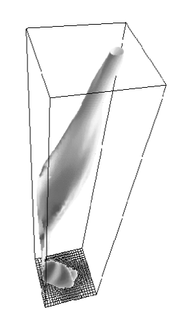
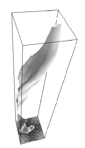
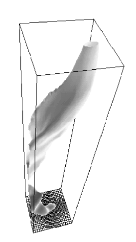
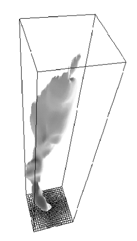
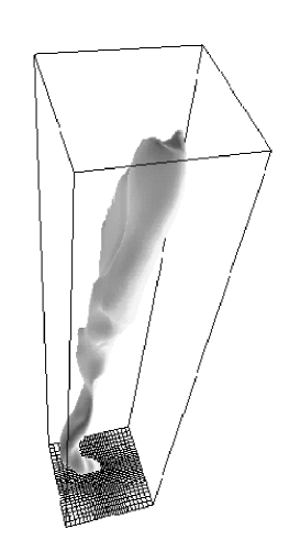
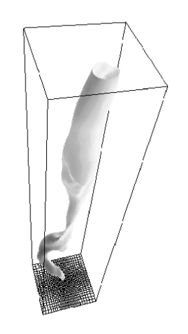
Figure 7: Isosurfaces of magnetic flux density for run 2. The snap shots are taken at $t=270,274,278,282,286,290$ starting at the upper left panel and ending at the lower right. The middle section of the flux tube is located off center and partly outside the test volume at first, but the non-axisymmetric distortion relaxes and the tube swings (clockwise) into a more axisymmetric configuration with a tightly wound spiral structure close to the disc surface. For clarity, only a narrow region of the computational domain centered around the $x$-axis is shown.

Though potentially disruptive events may be identified in the dynamics, these events are found only to generate filaments and cause non-destructive distortions of the jet beam. To monitor the onset and evolution of instabilities further, the magnetic field topology is investigated. Phenomenological investigations of the evolution of the field topology are carried out by visualizing isosurfaces of magnetic flux density. Fig. 7 shows the evolution of an isosurface of the magnetic flux density. The magnetic field is seen to develop a complex and highly non-axisymmetric structure, which relaxes periodically allowing the field to return to a less complex, more nearly cylindrical topology. In each such build-up/relaxation cycle several modes may be identified qualitatively such as the sausage instability and the elliptical ($|m|=2$) modes.

Figure 8: Total dissipation in a test volume for run 2 (upper panel) and run 2 (lower panel). The dissipation is integrated in a central volume of the box between $x=[0.7,38.1]$ and $y,z=[-4.7,4.7]$ and is normalized by the maximum value of the magnetic dissipation in each experiment. The solid lines are magnetic dissipation and the dashed lines are viscous dissipation.

The total viscous and magnetic dissipation as a function of time are shown in Fig. 8 for a test volume. In the initial phase the wound up field structure is building up and the magnetic dissipation is seen to increase sharply until $t\approx 100$. From the magnetic dissipation, several minor and a couple of major magnetic reconnection events are identified to occur in this region for run 2 (upper panel). The evolution of the magnetic field shown in Fig. 7 is seen to be connected to a significant increase in the magnetic dissipation. A slight increase is seen also in the viscous dissipation, indicating that a small fraction of the energy released by field re-organization is transferred into kinetic energy and subsequently dissipated.

The dissipation of the magnetic field does not match the Poynting flux into the test volume in general. The surplus of magnetic energy is partly used for driving the jet flow, as demonstrated in Sect. 3.1, and partly to build up the winding between relaxation events. In addition, there is a continuum of “background” magnetic dissipation between the relaxation events which may have important consequences for the jet stability. The significance of the magnetic diffusion varies in correspondence to e.g. the characteristic flow velocity as. Specifically, one expects in the $\beta_{\mathrm{i}}=10$ case (run 2) the characteristic (vertical) jet velocity to be less than in the $\beta_{\mathrm{i}}=5$ case (run 2) as noted in Sect. 3.1.1. Accordingly, the magnetic Reynolds number, $Re_{\mathrm{M}}=UL/\eta$, will be smaller in the weak field experiment and magnetic diffusion relatively more important. The magnetic diffusion is better capable of counter balancing the continual field winding and the build-up phase of the azimuthal field is prolonged. For the same reason the relaxation events themselves appear less violent, as seen by comparing the panels of Fig. 8, and will cause less destructive, more localized distortions of the flow.

The damping of the spiraling jet motion at heights where the jet is in general super-Alfvénic is related to what appears as field “unwinding” just outside of the super-Alfvénic central beam. Fig. 6 shows the orientation of the magnetic field in a cross section at $x\approx 20$ and illustrates the unwinding. The jet beam swings clockwise in the plot, and the change in field orientation is seen particularly on the front of the Alfvén surface in the direction of the (clockwise) spiral motion.

The unwinding of the field comes about as the spiral motion of the jet beam forces the wound up field into the ambient almost vertical field. The wound up field is oriented in a direction practically perpendicular to the ambient vertical field and reconnection occurs when these oppositely directed field lines are forced into a small region. This is seen as sheets of Joule dissipation marking the regions of magnetic diffusion at the jet flanks in the left panel of Fig. 9. The right panel of Fig. 9 shows such a sheet in more detail and the orientation of the field lines reconnecting. These magnetic reconnections, occurring in a “cocoon” surrounding the central jet beam, are the reason for the observed back-flow in Fig. 5 and the field unwinding in Fig. 6. More specifically, the upper right region of back-flow in Fig. 5 corresponds to where the reconnection events are expected to catapult gas backwards in this scenario. The gas at the “nose” of the Alfvén surface (at $y\approx 2$, $z\approx-1$) is accelerated oppositely, i.e. forward in the rotation direction and upwards. Also seen in left panel of Fig. 9 is a central region of significant magnetic dissipation. This is the region where reconnection occurs as a consequence of field interlocking resembling the scenario observed in experiments concerning coronal heating Galsgaard and Nordlund (1996). The right panel of Fig. 9 confirms this interpretation.

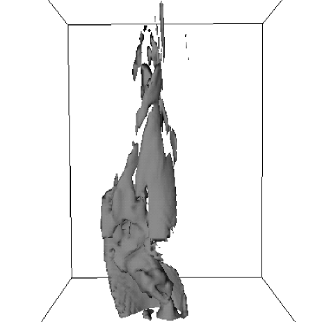
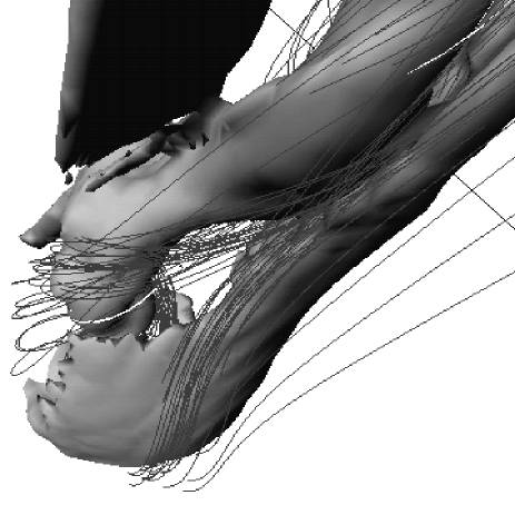
Figure 9: The left hand side panel shows isosurface of magnetic dissipation. The dissipation is seen to occur predominantly in two regions; in the central highly wound field region close to the rotation axis and in a “cocoon” at the jet flanks. The right hand side panel shows zoom-in on magnetic dissipation isosurfaces and inner wound up magnetic field field lines pressed towards the outer more vertical field. Both snap shots are from run 2 at $t=300$.

4 Discussion

Obviously, parameter space has not been probed in all detail in the work presented here. Issues which clearly need more attention in future work include the magnetic configuration, thermal conditions and mass loading. Probing other magnetic configurations would involve a significant change of the numerical code, whereas the inclusion of detailed cooling expressions would be straightforward Rögnvaldsson (1999); Rögnvaldsson et al. (2002). Magnetic field configurations which fan away from the jet axis in a more dipole like fashion may provide less stabilization high above the disc and far from the rotation axis. However, close to the central parts of the disc the field lines will, in a potential configuration as suggested by Cao and Spruit Cao and Spruit (1994), bend towards the jet axis as a function of height and not appear much different from the vertical configuration used in this work. The stabilization and collimation provided by the poloidal field may be reduced if the magnetic field is produced in a dynamo active disc. In such a scenario, Brandenburg et al. Bardou et al. (2001) have found that significant amounts of toroidal magnetic field are transported into the corona from the outer parts of the disc. This could seriously influence the stability.

Theoretically, the stability of twisted magnetic flux tubes is expected to depend on the diameter to length ratio (aspect ratio), such that relatively long tubes are most unstable. This is strictly valid only in the ideal magnetohydrodynamics case. In practice, the rate of magnetic dissipation tends to increase for more narrow tubes, which reduces the importance of the aspect ratio Galsgaard and Nordlund (1997). In the work presented here, no systematic change was found in the appearance of the jet when the aspect ratio of the experiment was changed (e.g. comparing runs 2, 2 and 2).

As a consequence of magnetic dissipation occurring primarily in two regions (cf. Sect. 3.2) the jet flow consists of a hot central beam, with temperature of the order of the virial temperature at the inner disc radius, and a hot cocoon. Hot jet flanks has been observed in YSO’s and are proposed to be generated by shocks associated with time variability and entrainment in the flow (e.g. HH47, Hartigan et al., 1993). The results presented in Sect. 3.2 suggest that magnetic dissipation may be a major additional mechanism for heating in this region.

Preliminary results (run 2) indicate that relatively cold disc outflow results in less distorted, more well-defined flows and relatively more dense jets. A similar result has been reported by Hardee et al. Hardee et al. (1997) who found dense jets to maintain a high-speed spine which prevents disruption of the internal jet structure though large helical and elliptical distortions were present. The experiment, as it is, is already suitable for addressing further which consequences the temperature of the disc outflow may have on the jet dynamics. However, further investigations with special emphasis on the transsonic region close to the disc surface are desirable to investigate the issues of mass loading and disc-jet interactions in general.

5 Summary and conclusions

A high order numerical scheme has successfully been adopted and a suitable mesh refinement specified. Initial conditions resembling previous axisymmetric numerical experiments have been chosen to ease comparison. The polytropic equation of state is only used initially, to prescribe the initial density distribution of the corona. The most important features that differ from previous jet experiments are:

• The model is three dimensional rather than axisymmetric. Due to the periodic boundaries, a cutoff of the disc at large radii is applied.

• The thermal energy equation is solved, with self-consistently computed heating by viscous and Joule dissipation.

• “Free” mass outflow from the disc, i.e. the mass flux is allowed to adjust self-consistently to the forces near the disc surface.

• Parameterized Poynting flux through the upper boundary, representing external work.

• The experiments have been evolved far beyond the initial transient, and display a quasistationary behavior, as evidenced for example by the nearly constant total energy flux.

The jet dynamics has been investigated by analyzing the mechanisms of energy conversion. The rotational energy of the disc is carried by the magnetic field into the corona and is first predominantly converted into kinetic energy. In the upper two thirds of the computational domain the magnetic energy is predominantly converted into thermal energy. General features predicted by steady state theory and axisymmetric numerical experiments, such as knot generation and terminal velocity dependency on the magnetic field strength have been confirmed in the relatively early and quiescent stages of the experiments. At later stages the flow becomes quite unsteady as instabilities set in, but no serious disruption of the flow occurs. The jet stability is found to be influenced by the magnetic dissipation — this has not previously been investigated in the context of jet flows. The main findings concerning magnetic dissipation are the following:

• The heating by magnetic dissipation is significant, and leads to jet temperatures of the order of the virial temperature of the innermost Kepler orbit.

• Magnetic reconnection occurs primarily in two regions: in a central region of the jet due to field interlocking and in a jet cocoon due to the spiraling motion of the jet beam forcing the wound up field into the ambient vertical field.

• Magnetic dissipation helps to prevent critical kinking, and the jet is able to sustain a quasistationary flow, with only limited excursions.

• Reconnection events are seen to result in mass ejection into the ambient medium and cause filament structures in the jet beam.

• Reconnection events are seen to significantly influence the dynamics at the jet flanks where deceleration and even back-flow can be found quite close to the central super-Alfvénic beam.

• Heating in the region just above the disc is likely to have a significant effect on the mass loading.