Detecting dark matter substructure spectroscopically in strong gravitational lenses

Abstract

The Cold Dark Matter (CDM) model for galaxy formation predicts that a significant fraction of mass in the dark matter haloes that surround $L\sim L_{*}$ galaxies is bound in substructures of mass $10^{4}$–$10^{7}\,{\rm M}_{\odot}$. The number of observable baryonic substructures (such as dwarf galaxies and globular clusters) falls short of these predictions by at least an order of magnitude. We present a method for searching for substructure in the haloes of gravitational lenses that produce multiple images of QSOs, such as 4-image Einstein Cross lenses. Current methods based on broadband flux ratios cannot cleanly distinguish between substructure, differential extinction, microlensing and, most importantly, ambiguities in the host lens model. These difficulties may be overcome by utilizing the prediction that when substructure is present, the magnification will be a function of source size. QSO broad line and narrow line emission regions are approximately $\sim 1$ pc and $>100$ pc in size, respectively. The radio emission region is typically intermediate to these and the continuum emission region is much smaller. When narrow line region (NLR) features are used as a normalisation, the relative intensity and equivalent width of broad line region (BLR) features will respectively reflect substructure-lensing and microlensing effects. Spectroscopic observations of just a few image pairs would probably be able to cleanly extract the desired substructure signature and distinguish it from microlensing – depending on the actual level of projected mass in substructure. In the rest-optical, the H$\beta$/[O III]  region is ideal, since the narrow wavelength range also largely eliminates differential reddening problems. In the rest-ultraviolet, the region longward and including Ly$\alpha$ may also work. Simulations of Q2237+030 are done as an example to determine the level of substructure that is detectable in this way, and possible systematic difficulties are discussed. This is an ideal experiment to be carried out with near-infrared integral field unit spectrographs on 8-m class telescopes, and will provide a fundamentally new probe of the internal structure of dark matter haloes.

1 Introduction

Galaxy formation models cast in a $\Lambda$CDM universe have experienced considerable success to date. With a fixed choice of cosmological parameters, it is possible to make specific predictions, for example based on N-body simulations, regarding the structure of individual dark matter haloes. One of the challenges in this field is to calculate the level of the continuously-infalling substructure that will survive within large haloes. Present N-body simulations indicate that there should be plentiful substructure in a $L_{*}$ galaxy’s halo, with masses above $10^{7}{\rm M}_{\odot}$; below this scale limitations in resolution becomes important. If these subhaloes contain stars, there should be significantly more dwarf galaxies near the Galaxy than are seen (Moore et al., 1999; Klypin et al., 2001). Various solutions to this excess problem have been proposed, including warm dark matter (which erases substructure on small scales; e.g. Avila-Reese et al. 2001); self-interacting dark matter (which causes subhaloes to evaporate; Spergel & Steinhardt 2000); and radiation-driven ionization of the intergalactic medium such that star formation in dwarf-size galaxies is suppressed at early epochs, as discussed in Somerville (2002), Bullock, Kravtsov & Weinberg (2001), and Klypin et al. (1999). If the substructure does exist, its gravitational influence should be detectable, and therefore this prediction of $\Lambda$CDM in particular may be tested. There is already some evidence in support of the need for substructure to explain the relative magnifications in strong lenses; disentangling its signature from other (equally interesting) effects is the scope of this paper.

From the positions of the images and lens galaxy of a 4-image lens system, a parametric smooth mass model for the lensing galaxy and halo can be computed (including external shear), along with predictions for the three independent flux ratios. Measuring deviations between the predictions and the (differential-reddening-corrected) observed integrated fluxes in real Einstein Cross lenses, provides a direct estimate of the surface density in substructure (Metcalf & Madau, 2001; Chiba, 2002; Metcalf & Zhao, 2002; Dalal & Kochanek, 2002). Substructure has long been considered a possible explanation for inconsistencies in the observed flux ratio of B1422$+$231 (Mao & Schneider, 1998). However, this approach has a vital flaw. The predicted flux ratios can be strongly dependent on the parametric lens models used, making any measurement of the mass fraction in substructure (e.g. Dalal & Kochanek, 2002) suspect. The observational technique proposed here largely avoids this important problem, as well as the problems of intrinsic variability (on the timescale of the typical time-delay between images), and the effects of microlensing, with the possible change of continuum slope as well as intensity.

In §2 the main features of substructure and its lensing effects are summarized. Simulations demonstrating the importance of source-size on magnification are presented in §2.3, for a specific lens, Q2237+030. The spectroscopic approach proposed here is discussed in §3, with the most difficult problems and their possible solutions addressed. In §4 we discuss selection criteria for lens candidates for this experiment, as well as modes of observations that would be sufficient for obtaining results. The main conclusions are summarized in §5. In the Appendix an estimate of the observational uncertainties is calculated. All cosmological calculations are carried out for a $\Lambda$CDM cosmology, with $\Omega_{\Lambda}=0.7$, $\Omega_{0}=0.3$, though none of the arguments (except the level of substructure one might expect) depend strongly on this choice. The Hubble parameter is $\mbox{H}_{0}=65\,h_{65}\mbox{ km s${}^{-1}$}\mbox{ Mpc}^{-1}$.

2 Substructure & Gravitational Lens Models

2.1 substructure and small-mass dark matter haloes

The highest-resolution N-body simulations of structure formation are currently limited to $\sim 10^{6}{\rm M}_{\odot}$ particles (e.g. Moore et al., 1999). Down to the scale of 10 particles ($\sim 10^{7}{\rm M}_{\odot}$) there is clear evidence for surviving substructure within large dark matter haloes with a power-law mass function, $dN/dm\propto m^{-\alpha}$, where $\alpha\simeq 1.91$. For observed dwarf galaxies, $\alpha\simeq 2.35$ (Klypin et al., 2001). In these simulations there is a continuous process of infall and merging working against tidal stripping and dynamical friction to maintain the substructure population. Within the virial radius of a galactic halo, about $10$–$15$% of the mass is in structure of mass $\lower 2.15277pt\hbox{$\;\buildrel>\over{\sim}\;$}10^{7}{\rm M}_{\odot}$. Analytic arguments suggest that future simulations with a larger dynamic range will find that substructure survives down to far smaller masses than are currently accessible by direct computation (Metcalf & Madau, 2001).

In addition to the substructure inside the primary lens, there will also be small haloes in intergalactic space in front of and behind the primary lens. Zhao & Metcalf (2002; in prep.) show that the importance of these two populations to compound lensing is approximately equal, if the tidal destruction of haloes within the lens is negligible. Tidal destruction will increase the relative importance of intergalactic haloes although the importance of this cannot yet be accurately quantified. Despite this, in our estimates and simulations we treat all the haloes as if they are at the same redshift as the primary lens. Since the strength of a lens of fixed mass reaches a maximum when the lens is half way to the source, measured in angular size distance, and the primary lens is usually near this point, an estimate of the surface density in substructure under this simplification will be an estimate of the minimum density required to produce the observed lensing effects.

The importance of haloes to lensing is strongly dependent on their internal structure. To quantify the internal structure in some of the estimates given below, we use the parameter $\gamma(r)\equiv d\ln M(r)/d\ln r$, where $M(r)$ is the mass of the halo within a projected radius of $r$. The tidal radius of a subhalo is set by the requirement that the average density within that radius be proportional to the average density of the host halo within the orbit of the subclump – the constant of proportionality depends on the structure of the host. This means that the average density $\overline{\rho}_{c}=3m/4\pi r(m)^{3}$, where $r(m)$ is the radius of a subhalo, will be independent of mass. Additionally, in the hierarchical structure formation model, the initial density of a halo is proportional to the average density of the universe at the time when the halo first collapsed. In the CDM model all the small-mass haloes of interest here are almost coeval. This results in the same conclusion for the intergalactic haloes as for the subhaloes – $\overline{\rho}_{c}$ is independent of mass although it may have a different value for the two populations. We will take $\overline{\rho}_{c}$ to be a free parameter in our discussions.

2.2 the influence of source size on lensing

We can make some estimates for how compound lensing will be affected by the size of the source QSO using the simple model of substructure outlined above. Let us brake the magnification matrix, $A_{ij}$, into a contribution from the smooth lens and a perturbation caused by the small clumps – $A_{ij}=A^{o}_{ij}+\delta A_{ij}$. Let us say a clump will have a significant influence on the magnification if $\delta A_{ij}$ is of order $\epsilon$ or larger. The value of $\epsilon$ will depend on the magnification caused by the unperturbed smooth lens ($\delta\mu/\mu\sim\mu_{o}\epsilon$ where $\mu_{o}$ is the smooth lens magnification). The magnification of a source with finite size is the point-source magnification integrated over the area of the image. Because of this, a finite source sees a magnification that is smoothed on the scale of its own size. For a halo to have an influence, the region where its contribution to the magnification matrix is greater than $\epsilon$ must be larger than the image of the source. If we take the physical size scale of the source to be $\ell_{s}$, this requirement puts a lower limit on the mass of haloes that can be important for lensing:

$$m_{c}=\left[\left(\frac{\epsilon\pi\Sigma_{c}}{1+\gamma}\right)\left(\frac{D_{l}\ell_{s}}{D_{s}}\right)^{2-\gamma}\left(\frac{4\pi}{3}\overline{\rho}_{c}\right)^{-\gamma/3}\right]^{3/(3-\gamma)}.$$ (1)

where the critical density is $\Sigma_{c}=(4\pi GD_{l}D_{ls}/c^{2}D_{s})^{-1}$ and the angular size distances to the lens, source, and from the lens to the source are denoted by $D_{l}$, $D_{s}$, and $D_{\rm ls}$, respectively. The logarithmic slope $\gamma$ is evaluated at the radius where $\delta A(r)\simeq\epsilon$.

It is useful to put some typical numbers into Eqn. 1. Consider a source at $z_{s}=2$ and a lens at $z_{l}=0.5$. In this case $\Sigma_{c}=1.93\times 10^{9}h_{65}{\rm M}_{\odot}/{\rm kpc}^{2}$ and $D_{l}/D_{s}=0.73$. For a point-mass (the most condensed possible halo), $\gamma=0$ and

$$m_{c}\simeq 3.2\times 10^{3}\epsilon h_{65}\left(\frac{\ell_{s}}{\mbox{ pc}}\right)^{2}{\rm M}_{\odot}~{}~{}~{}\mbox{(point-mass lens)}.$$ (2)

Figure 1: The minimum mass of a small halo that can have an influence on the compound lensing as a function of the source size. The solid line is from Eqn. 2. The dashed line is Eqn. 3 with $R=1\mbox{ kpc}$ and $\sigma_{h}=200\mbox{ km s${}^{-1}$}$. In both cases $h_{65}=1$ and $\epsilon=0.1$. If the magnification is high ($\mu\lower 1.72221pt\hbox{$\;\buildrel>\over{\sim}\;$}10$), $\epsilon=0.01$ would be more appropriate. The general size range for different emission regions of a QSO are labelled (BLR – broad line region; NLR – narrow line region). The central accretion disc of a QSO which is believed to be the source of the continuum emission has a scale of $10^{-4}-10^{-3}\mbox{ pc}$; off the scale to the left.

For less condensed haloes we must make an assumption about their internal density, $\overline{\rho}_{c}$. The characteristic density of the intergalactic haloes, $\overline{\rho}_{c}$, is set by the process of structure formation at high redshift. If these haloes fall into a host lens they will remain intact until the average density of the halo within their orbit, $\overline{\rho}_{h}(R)$, becomes of order the density of the subhalo, then it will be tidally stripped. If all the subhaloes are tidally truncated, their density can be calculated from the average interior density profile of the host, $\overline{\rho}_{h}(R)$. If the host is modeled as a singular isothermal sphere (SIS), $\overline{\rho}_{c}=2\overline{\rho}_{h}(R)$. This results in a cutoff mass of

$$m_{c}\simeq 1.7\times 10^{4}{\rm M}_{\odot}\left(\epsilon h_{65}\frac{\ell_{s}}{\rm pc}\right)^{3/2}\frac{200}{\sigma_{h}}\frac{\rm km}{{\rm s}}\frac{R}{\rm kpc}~{}\mbox{(SIS)},$$ (3)

where $\sigma_{h}$ is the velocity dispersion of the host lens. The haloes could be denser than assumed here if they were born denser, or they could be less dense if they were born less dense and primarily reside outside of the primary lens. Since no accurate simulations of structure formation at these small mass scales have been done, we will take the above estimates as benchmarks for our discussions.

The estimates of $m_{c}$ are plotted in Figure 1 as a function of source size along with the approximate size scales for different emission regions of a QSO as discussed in section 3.1. The image of a source of a given size will be affected by halo masses above this limit. For example, the image of a 1 pc source will reflect the influence of haloes with $m\lower 2.15277pt\hbox{$\;\buildrel>\over{\sim}\;$}10^{3}{\rm M}_{\odot}$ while the image of a 100 pc source will only be affected by haloes with $m\lower 2.15277pt\hbox{$\;\buildrel>\over{\sim}\;$}10^{6}{\rm M}_{\odot}$. For source sizes below $\sim 10^{-2}\mbox{ pc}$ (such as the accretion disc of a QSO), $m_{c}$ is less than a solar mass, making microlensing by ordinary stars possible. Figure 2 shows $m_{c}$ as a function of lens redshift. The drop in $m_{c}$ near $z_{l}=0$ in Figure 2 for the point masses is somewhat misleading here because the Einstein radius becomes very small near $z_{l}=0$ making these cases extremely rare. The value of $m_{c}$ for any realistic substructures lies somewhere between its value for point mass lenses and SIS lenses.

This mass cutoff alone indicates that the magnification should be a strong function of source size if there is a large population of haloes with $m\lower 2.15277pt\hbox{$\;\buildrel<\over{\sim}\;$}10^{7}{\rm M}_{\odot}$. There are other factors that influence how magnification will depend on source size. Larger sources are more likely to be eclipsed by rarer, larger haloes. On the other hand, if the haloes have high density cusps in their centers – as expected from simulations – smaller sources can reach higher magnifications. To determine accurately how the magnification distribution will depend on source size and halo mass distribution requires numerical simulations.

Figure 2: The minimum lensing mass as a function of the source size as defined in Eqn 1. The solid curves are for point mass substructures and the dashed are for singular isothermal spheres. The lower of each set of curves are for a source size of $\ell_{s}=1\mbox{ pc}$ and the upper for $\ell_{s}=1\mbox{ pc}$. The curves that stop at $z_{l}=1$ are for source redshift $z_{s}=1$. The others are for $z_{s}=2$. The SIS are tidally truncated with $R=1\mbox{ kpc}$. A realistic case would probably lie somewhere between the point mass and the SIS curves of each type. In all cases, $h_{65}=1$ and $\epsilon=0.1$.

2.3 lensing simulations: Q2237+030

We take the image positions and lens galaxy position of the 4-image QSO lens system Q2237+030 and fit a elliptical power-law plus shear model to them for the smooth lens component (see Metcalf & Zhao 2002 for details). To calculate the magnifications with substructure, an improved version of the ray tracing code used by Metcalf & Madau (2001) is used. The lensing equation is solved to obtain the source position for each point on a coarse grid surrounding the unperturbed image position. The closest grid point to image position is found and a new smaller grid is set up around that point. This process is repeated until the image takes up a large fraction of the grid and the desired accuracy is reached (usually $\delta\mu/\mu=10^{-3}$). This grid-refinement technique allows us to achieve the large dynamical range required to calculate the magnifications of sources with sizes ranging from less than 1 pc to several hundred pc while keeping the substructure fixed.

The substructure is modeled as singular isothermal spheres truncated such that $\overline{\rho}_{c}=6.9{\rm M}_{\odot}\mbox{ pc}^{-3}$ and with a mass function of $dN/dm\propto m^{-2}$. The total surface density in substructures with $10^{3}{\rm M}_{\odot}<m<10^{6}{\rm M}_{\odot}$ is fixed at 10% of the total surface density according to the smooth model. Random realizations of the masses and positions of the subclumps are made and the magnifications with several different sources are calculated in each one.

Figure 3: Simulated magnification ratios between image B and image D of quad-lens Q2237+030 using two different source sizes. Each circle is a different realization of the substructure. There are 1 000 realizations shown. Without substructure, $\Delta m_{24}$ should not depend on source-size in this range so all the points would be on the 45^∘ line shown. The range of ratios along the 45^∘ line is larger, but excursions in this direction can be degenerate with the smooth lens model. Excursions perpendicular to the line unambiguously indicate small-scale structure.

Figure 4: The differences in magnification ratios between image A and image D of quad lens Q2237+030 using three different source sizes (1 pc, 10 pc and 100 pc). A smooth, substructure-free lens would predict that the three magnification ratios would be very close to equal, the center of the plot. These are the same 1 000 realizations as in Figure 3. One quarter of the realizations have $|\Delta m_{14}(10\mbox{ pc})-\Delta m_{14}(1\mbox{ pc})|>0.05\mbox{ mag}$ and one quarter of them have $|\Delta m_{14}(1\mbox{ pc})-\Delta m_{14}(100\mbox{ pc})|>0.18\mbox{ mag}$.

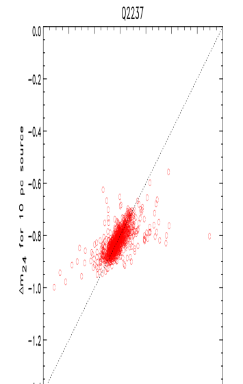
Figure 3 shows the flux ratio, measured in magnitudes, of image A to image D (marked ‘1’ and ‘2’) in Q2237+030 for 1 000 realizations of the substructure. The ratios for source sizes of 1 pc and 10 pc are shown. If there were not a substantial number of haloes with mass less than $\sim 10^{6}{\rm M}_{\odot}$, we would expect these two ratios to be equal and the circles in the plot to lie on the diagonal line. No smooth model can account for points being off this line.

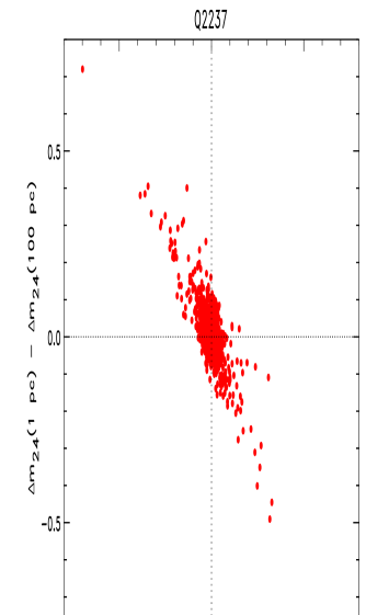
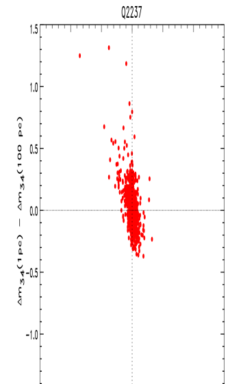
Figures 4 through 6 show simulations of all three magnification ratios for Q2237+030. In each case, three different source sizes are used. If the lens were smooth all three magnification ratios would be the same and all the dots in the figures would be located precisely at the origins in these plots. Figure 7 shows the cumulative distribution of the simulated differential magnification ratios. We can see that in half of the cases the differential magnification ratio is larger than 0.1 mag. If this level of measurement accuracy can be attained, only 1–3 lens systems will be required to rule out this level of substructure.

Figure 5: Same as in Figure 4, but for images B and image D of Q2237+030. In this case one quarter of the realizations have $|\Delta m_{24}(10\mbox{ pc})-\Delta m_{24}(1\mbox{ pc})|>0.05\mbox{ mag}$ and one quarter of them have $|\Delta m_{24}(1\mbox{ pc})-\Delta m_{24}(100\mbox{ pc})|>0.07\mbox{ mag}$.

Our model for Q2237+030 predicts magnifications that are relatively modest ($\mu_{A}=2.28$, $\mu_{B}=-0.939$, $\mu_{C}=2.047$, $\mu_{D}=-2.005$). Since the substructure has an influence on the magnification that is proportional to the smooth components magnification ($\delta\mu\propto\mu_{o}^{2}$), we expect that these results are fairly conservative. Some published models for other quad lenses predict magnifications as large as 100.

Figure 6: Same as in Figure 4 but for images C and image D of Q2237+030. In this case one quarter of the realizations have $|\Delta m_{34}(10\mbox{ pc})-\Delta m_{34}(1\mbox{ pc})|>0.05\mbox{ mag}$ and one quarter of them have $|\Delta m_{34}(1\mbox{ pc})-\Delta m_{34}(100\mbox{ pc})|>0.17\mbox{ mag}$.

We can see from these simulations that it is possible to detect substructure, or intergalactic dark haloes, in a way that is independent of any lens model, if we can measure the flux ratios to $\sim 0.1$ mag for sources that differ in size by a factor of ten and are centered on the same object. This can be done with a very small number of lens systems. Interpreting the results in terms of the fraction of mass in small mass haloes and the slope of the mass function will require some modeling of the smooth lens component, but even then the results will be much less model dependent than the more traditional method based on single broad-band measurements of the flux ratios.

Figure 7: Here is a histogram the cumulative distribution of the differential magnification for the three independent ratios in Q2237+030. On the y-axis is the fraction of simulations out of 1 000. The source sizes used are 1 pc and 100 pc to reflect the approximate sizes of the BLR and the NLR, respectively.

3 The Spectroscopic Approach

3.1 the internal structure of QSOs – a sketch

In QSO spectra, the ‘narrow line region’ (NLR) emission lines (e.g. [O III] $\lambda\lambda 4959,5007$) do not vary in flux significantly over the time span of several years (Kaspi et al., 1996). For this reason, they have been used for calibration in long-term spectroscopic monitoring observations of low redshift QSOs for reverberation mapping experiments, by which the time delays between features of different ionization states may in principle be used to map all the components that make up QSOs (Peterson, 1993). Photo-ionization arguments and cases where the NLR-emitting region is imaged directly, indicate that the size of the NLR extends out to 100-1000 pc.

In the full unification picture for active galactic nuclei (AGN) including QSOs, the variability timescales of different spectroscopic features, and the time delays between them, are used to map out the size and structure of different components with very different characteristics (c.f. Antonucci, 1993). The basic idea consists of a supermassive black hole (M${}_{bh}>10^{6}$M_⊙) in the core, surrounded by an accretion disc, which produces the nearly flat-spectrum continuum light seen. The continuum flux varies on very short timescales, less than a day, and so must be very compact (around 100 AU or $\sim 5\times 10^{-4}$ pc). It is also known to be microlensed in the case of Q3327+030 which puts an upper limit of 2 000 AU on its size (Yonehara, 2001, and references therein). Beyond that, there are permitted lines such as the Balmer-series lines that are very broad ($v_{\rm FWHM}>10^{3}$ km s^-1) due to gravitationally-induced motions. The characteristic size of this ‘broad line region’ (BLR) apparently scales with the intrinsic luminosity of the host QSO (and therefore with the mass of the central black hole; Kaspi et al. 1996; Wandel 1999), such that in luminous QSOs (as opposed to, e.g., Seyfert 1’s), the size of the BLR is on the order of six light-months (or $\sim 0.3$ pc). According to long-term studies of QSOs, the typical (rest-frame) flux variations in the QSO continuum are on the order of 10–70% (though occasional fluctuations as high as $\sim 50\times$ are possible; Ulrich et al. 1997), while the BLR variations are smaller by a factor of 2–4 (Maoz et al., 1994). In the observed frame, these timescales are stretched by an additional factor of (1+$z_{s}$).

Figure 8: In the rest-optical, the shown rest-wavelength region (from the SDSS QSO template, Vanden Berk et al. 2001), includes the NLR [O III] $\lambda\lambda 4959,5007$ and the BLR H$\beta$ emission features. Where the NLR emission line is used for normalising the spectra of each lensed image, any residual in the relative intensity of the BLR H$\beta$ emission lines after accounting for the relative magnification in the relevant gravitational lens model, will most likely be due to compound-lensing due to substructure in the foreground ‘smooth’ lens gravitational potential, whereas intensity variations in the continuum will be due to a combination of substructure- and micro-lensing, and other effects as discussed in the text.

There is some evidence for anti-correlations between the rest-ultraviolet continuum flux and the equivalent width of certain emission lines (Baldwin 1977; Green et al. 2001), which may also be related to the correlation between the central black hole mass and the continuum flux (Wandel, 1999). The general trend claimed, is that the more luminous QSOs have less pronounced broad-line emission line components, the [O III]/H$\beta$ central-flux ratio is small, and the rest-ultraviolet and -optical Fe II multiplet emission lines are more prominent, obfuscating the ‘true’ local continuum level that underlies these emission lines. There is strong (brightening) evolution with redshift observed in the luminosity function of QSOs, so that in general, high-redshift optically-selected QSOs are less likely to have strong [O III] emission. The QSO templates from the Large Bright QSO Survey (LBQS; Francis et al. 1992) and the Sloan Digital Sky Survey (SDSS; Vanden Berk et al. 2001) are compiled from objects over a broad range of redshifts, relatively few at $z<1$ (where the rest-optical window around H$\beta$ is still visible). Therefore, the H$\beta$ region in these templates is drawn from objects that are relatively local and of lower luminosity, and so generally show a misleadingly large [O III]/H$\beta$ ratio, if they are to be applied to higher-redshift considerations.

The only definite way to determine the characteristics of a particular system is by direct observations in the rest-optical. For example, in the case of B1422$+$231 at $z_{s}=3.62$, Murayama et al. (1999) find that the Fe II $\lambda\lambda 4434$-$4684$ emission is relatively weak compared to H$\beta$, similar to lower-redshift QSOs.

3.2 the spectroscopic approach for substructure

Consider a case where the spectrum of all images in an Einstein Cross are obtained, in a wavelength range where both NLR and BLR emission features are visible at high signal-to-noise (SNR $>\!\!>$ 10), and with sufficient spectral resolution to clearly resolve the shapes of the lines ($v_{res}$$\;\buildrel<\over{\sim}\;$$200$ km s^-1). The NLR emission lines are used to normalise the spectra to each other, and we wish to attempt to disentangle the substructure signature from other effects. There are several systematic errors to consider.

Differential Reddening – As each lensed image follows a different line of sight through the lensing galaxy, if the gas and dust in the galaxy are sufficiently patchy or position dependent, it is possible that there will be differential reddening that may affect the measured continuum slope and relative emission line fluxes. Falco et al. (1999) measured the $\Delta\,E(B-V)$ in 23 lens galaxies using HST broadband colours, under the (optimistic) assumption that variability and microlensing were not important. In recent broadband-magnitude-based substructure estimates, the colour corrections estimated by the above work were applied, which, in light of the possibility of microlensing, may introduce unquantifiably systematic errors for any one system. In the spectroscopic approach, choosing NLR and BLR emission lines that are close in wavelength, the differential reddening is very small. Taking the median value of $\Delta\,E(B-V)=0.04$ mag in the Falco et al. (1999) optically-selected sample, and assuming a MWG-type extinction law (Cardelli et al., 1989), we estimate that flux ratio between [O III] $\lambda\lambda 4959,5007$ and H$\beta$ for $z_{s}=3$ and $z_{l}=1$ will vary by less than 0.07% and can therefore be ignored. For comparison, between [O II] $\lambda 3727$ and Mg II $\lambda 2800$ the variation will be about 1.4%.

Microlensing – Some microlensing by stars probably occurs in most lenses, but it is most clearly seen in quadruple lenses (Witt, Mao & Schechter, 1995, and citations thereof). Microlensing events last months or years, much longer than the time delay between images, but (especially at caustic crossings, which can occur quickly) can magnify an image by as much as a whole magnitude (e.g. Witt, Mao & Schechter, 1995). For super-microarcsec sources, like the BLR of a QSO, stellar microlensing is insignificant (Figure 1), but for smaller sources, like the more compact QSO non-stellar continuum, microlensing will affect the magnification. Hence, observations of the relative flux of the broad component of BLR lines in the images (e.g. after any narrow component has been fit out) will reveal the effects of lensing by CDM substructure alone, while their equivalent widths can be used to probe ongoing microlensing because they are measured relative to the continuum (McLeod et al., 1998). Thus, in a spectroscopic experiment as we have described, it would be possible to place a limit on microlensing and substructure lensing simultaneously.

If the QSO accretion disc has a steep temperature gradient, it is also possible for microlensing of the disc to produce wavelength-dependent magnification in the continuum of the affected image (as seen in HE $1104$–$1805$ by Courbin et al. 2000). This does not affect the BLR emission line fluxes, as compared against NLR lines, though it is also spectacular evidence for microlensing.

Intrinsic QSO Variability – The continuum flux variations in QSOs can be quite large and rapid, on timescales comparable to the time delay between images. The BLR emission line fluxes vary less dramatically, and only reflect the more pronounced fluctuations seen in the continuum, with a several-month time-lag in the rest frame. For source redshifts $z_{s}\approx 2$, the observed-frame time-lag becomes close to a year. As long as variations in the observed frame happen on timescales that are significantly longer than the time delay between images in a given lens system, using the BLR lines as a substructure probe should be robust.

4 Discussion

The ideal target is a four-image lensed QSO with an exceptionally well-determined (smooth) gravitational lens model, at a redshift such that the ideal H$\beta$/[O III] features are redshifted into convenient observable windows, unobscured by strong atmospheric emission bands. It is also desirable for the target QSO to have a high [O III]/H$\beta$ ratio, which typically also means that the H$\beta$ emission will be dominated by its BLR component, and also that the Fe II complex shortward of H$\beta$ will be weak, such that the underlying local continuum can be measured securely. The redshifts of the sources in most Einstein Crosses are known; their H$\beta$/[O III] features have only been measured, at low signal-to-noise, in very few cases. Therefore, in many cases exploratory observations may be necessary. Several systems will need to be studied in detail in any case, to build up the statistics needed for a definitive measurement.

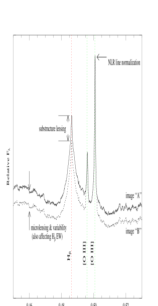
As illustrated in Figure 8, in the rest-optical the [O III] $\lambda\lambda 4959,5007$ and H$\beta$ lines are close, but separated enough to be distinguishable at even moderate spectral resolution. At the redshifts of most gravitationally lensed QSOs (typically $z>2$), these features are shifted into one of the near-infrared windows at $\lambda>1\mu$m ($JHK$).

In the Appendix we investigate the expected statistical uncertainties in a measurement the ratios between lines and continuum. Based on a ‘typical’ QSO (e.g the SDSS template; Vanden Berk et al. 2001), the BLR to NLR emission-line ratio may be measured with an error of $\sigma_{\omega}\simeq 0.3/SNR$, where $SNR$ signal to noise ratio per resolution element with which the continuum is measured. Likewise, the continuum to NLR emission-line ratio can be measured with error $\sigma_{c}\simeq 10/SNR$. If in the continuum a $SNR\sim 100$ is achieved, then based on our simulations in §2.3 (with $\sim 10\%$ of the surface density in compact objects below $\sim 10^{6}{\rm M}_{\odot}$, as seems to be the case in $\Lambda$CDM), then we expect the line ratios between the images of a typical lens system to differ by an amount larger than the measurement error. The situation is actually a bit better than this because all the images can be used to fit the full line shapes simultaneously. Observations of additional lens system can be used to improve the sensitivity to the substructure mass fraction.

These levels of the SNR are easily feasible with 8-m class telescopes for many Einstein Crosses and relatively moderate amounts of observing time. For instance, the Einstein Cross Q2237+030 QSO images, at $z_{s}=1.69$, have infrared magnitudes of $H\approx 16.0$ (from CASTLES). With 3 hours of integration on an 8-m telescope with $v_{res}$$\;\buildrel<\over{\sim}\;$$50$ km s^-1, the relevant part of the continuum, will be detected with $SNR$$\;\buildrel>\over{\sim}\;$$100$.

5 Conclusions

In $\Lambda$CDM, a significant fraction of the dark matter in $L\sim\,L_{*}$ galaxy haloes is in coherent substructure, with masses of $10^{4}$–$10^{8}$ M_⊙, which does not seem to have baryonic, or at any rate luminous, counterparts. The substructure and small-scale intergalactic structure should be detectable by its gravitational signature in multiply-imaged QSOs. If such substructure is sufficiently abundant along the images’ lines of sight, the light from different emission regions of a QSO will be magnified differently. This would be a model independent signature of small scale substructure.

Broadband photometry is primarily a measurement of the continuum flux, which is affected by rapid fluctuations intrinsic to the QSO, and by microlensing caused by stars. The magnitudes of both of these effects are at least comparably to what substructure is expected to produce, and conventionally can only be tracked by extensive monitoring.

We propose that these fundamental limitations can be largely overcome by obtaining high signal to noise spectra ($SNR\lower 2.15277pt\hbox{$\;\buildrel>\over{\sim}\;$}100$) of two or all lensed images simultaneously, that include prominent NLR and BLR features. The NLR features are used to normalise the spectra to each other, and then the relative fluxes of the BLR line(s) should be primarily due to substructure differential magnification. Intrinsic variability in BLR lines is observed to amount to $\sim 10$–$35$%, but relatively smoothly, and on characteristic timescales of greater than six months in the rest frame (and 1+$z_{s}$ times longer in our observed frame). Compared to the time delay of only days or weeks between the images in typical Einstein Crosses, the intrinsic BLR fluxes can be assumed to be constant.

The ideal setup is with an integral field unit (IFU) in the near-infrared (NIR), targeting the rest-optical [O III] & H$\beta$ emission lines. With the IFU setup, it is possible to get high-quality spectra of all images (and possibly of the lens, as well), simultaneously. The alternative of a set of longslit observations can be made more efficient by aligning on pairs of lens images, positioning the slit close to the parallactic angle to minimize the effects of differential refraction. Efficient implementation will require an 8-m class telescope, with excellent seeing conditions ($\sim 0.6^{\prime\prime}$), perhaps with adaptive optics.

This experiment will provide a concrete measurement, or at least place a severe upper limit on the fraction of dark-matter substructure in galaxy haloes and intergalactic space as predicted by the popular CDM models of structure formation. These models are presently in a state of crisis because of the lack of observations of this substructure.

APPENDIX

Expected Uncertainties in line strength ratios

We wish to estimate how well the ratio of the strengths of the broad and narrow lines can be measured. To do this we will model the flux in the $i$th resolution of the spectrum as consisting of four contributions: the broad lines ($\omega^{\prime}W^{b}_{i}(\Delta_{b})$), the narrow lines ($f^{n}W^{n}_{i}(\Delta_{n})$), the continuum emission ($c^{\prime}C_{i}$) and instrumental noise ($N_{i}$). The functions $W^{b}_{i}$, $W^{n}_{i}$ and $C_{i}$ are normalised so that their sum over all resolution elements is one and their widths (and perhaps some other shape parameters) are $\Delta_{b}$ and $\Delta_{n}$. We are interested in the ratio $\omega\equiv\omega^{\prime}/f^{n}$. The flux is then

$$F_{i}=I_{i}f^{n}(\omega W^{b}_{i}(\Delta_{b})+W^{n}_{i}(\Delta_{n})+cC_{i})+N_{i}$$ (A1)

where $I_{i}$ is the extinction and $c=c^{\prime}/f^{n}$. We will rewrite the extinction curve as $I_{i}f^{n}=ah_{i}$ with the normalisation $\sum_{i}h_{i}W^{n}_{i}=1$ so that $a$ is the total flux in the narrow lines after extinction correction. If we assume Gaussian, uncorrelated noise the log of the likelihood function will be

$$-\ln{\mathcal{L}}=\sum_{i}\frac{1}{2\sigma_{i}^{2}}\left[ah_{i}(\omega W^{b}_{i}(\Delta_{b})+W^{n}_{i}(\Delta_{n})+cC_{i})-F_{i}\right]^{2}+\ln(2\pi\sigma_{i}^{2})/2.$$ (A2)

For our present purposes it is convenient to replace the sum over resolution elements in (A2) with an integral over wavelength by making the substitution $\sum_{i}\rightarrow\delta\lambda^{-1}\int d\lambda$ where $\delta\lambda$ is the width in wavelength of the resolution elements. We will assume that the noise is constant over the wavelength range considered and given by $\sigma_{n}$.

The Fisher information matrix is defined as

$$F_{p_{1}p_{2}}=-\left\langle\frac{\partial^{2}\ln{\mathcal{L}}}{\partial p_{1}\partial p_{2}}\right\rangle$$ (A3)

where $p_{1}$ and $p_{2}$ are two parameters that are to be constrained by the measurements. The variance of the minimum variance unbiased estimator of a parameter $p$ is given by the Cramer-Rao bound

$$\sigma^{2}_{p}=(F^{-1})_{pp}.$$ (A4)

To calculate this we must identify the parameters in (A2) that are to be fit to the spectrum. The region of the spectrum we are interested in, shown in Figure 8, is relatively small compared to the complete spectrum and it is in region where the continuum has a shallow minimum in template QSO spectra(Vanden Berk et al., 2001). For simplicity we will approximate the extinction, $h(\lambda)$, and continuum, $C(\lambda)$, as constant over the region of interest, but we will allow their normalisations to vary. Formally, this is a valid approximation if $d\ln C(\lambda)/d\lambda,d\ln h(\lambda)/d\lambda\ll 1/\Delta\lambda$ where $\Delta\lambda$ is the range of wavelength considered. We will also assume that the redshift of the QSO is well established so that the positions of all lines are known. This leaves five parameters to be determined – $\omega$, $c$, $a$, $\Delta_{n}$ and $\Delta_{b}$. There are then 15 independent elements in the Fisher matrix which we calculate. In general the profiles of the lines are functions of multiple parameters which could be added to the list, but for simplicity we will leave these out here and take the lines to be Gaussian. Once these matrix elements are calculated the matrix can be inverted numerically.

It is convenient to express error estimates in terms of the signal to noise per resolution element with which the continuum can be measured. In our parameterization this is

$$\sigma_{o}\equiv\frac{\sigma_{n}\Delta\lambda}{ac\delta\lambda}.$$ (A5)

A noise level of $\sigma_{o}\sim 0.01$ may be reasonable. Table 1 shows the estimated errors for several choices of fiducial parameters. The ratio of the continuum flux within the range $\Delta\lambda$ to the narrow line flux, $c$, is estimated from the height of the narrow lines relative to the continuum in composite spectra (Vanden Berk et al., 2001). We use only H$\beta$ and [O III] $\lambda\lambda 4959,5007$ for the estimates and assume that no lines overlap except the BL and NL H$\beta$. The source is at $z_{s}=2$.

Parameter Values							Estimated Errors in units of $\sigma_{o}$
$R^{\spadesuit}$	$\Delta\lambda^{\dagger}$	$\omega$	$c$	$acC(\lambda)^{\ddagger}$	$\Delta_{n}$	$\Delta_{b}$	$\sigma_{\omega}$	$\sigma_{c}$	$\sigma_{a}/a$	$\sigma_{\Delta_{n}}/\Delta_{n}$	$\sigma_{\Delta_{b}}/\Delta_{b}$
———————————————————————-							—————————————————–
3000	50,000	1.0	22.2	$1.7\times 10^{-16}$	300	5,000	0.255	13.1	0.538	0.531	1.19
3000	100,000	1.0	19.9	$1.7\times 10^{-16}$	500	10,000	0.148	6.88	0.309	0.308	0.746

^♠ Resolution of spectrograph, $R=\lambda_{o}/\Delta\lambda$.
^† $\Delta\lambda$, $\Delta_{n}$ and $\Delta_{b}$ are expressed in km/s.
^‡The continuum flux in $\mbox{erg}\mbox{ cm}^{-1}\mbox{s}^{-1}\mbox{\AA}^{-1}$.

Table 1:

In this analysis we have ignored the noise associated with subtracting the sky and the absolute flux calibration. This might interfere with the measurement of the total flux from the NL, $a$, but should not seriously interfere with measurements of the ratios between NL and BL or between the continuum and the NL. We also ignored the fitting of the ratios between NLs which we do not think would affect our estimates by much. The line shape estimates are relatively statistically independent from the line ratio estimates so we also do not expect that having more complicated line shapes would greatly change our estimates.

References

- Antonucci (1993) Antonucci R., 1993, ARA&A, 31, 473
- Avila-Reese et al. (2001) Avila-Reese V., Colín P., Valenzuela O., D’Onghia E., Firmani C., 2001, ApJ, 559, 516
- Baldwin (1977) Baldwin J. A., 1977, ApJ, 214, 679
- Bullock et al. (2001) Bullock J. S., Kravtsov A. V., Weinberg D. H., 2001, ApJ, 548, 33
- Cardelli et al. (1989) Cardelli J. A., Clayton G. C., Mathis J. S., 1989, ApJ, 345, 245
- Chiba (2002) Chiba M., 2002, ApJ, 565, 17
- Courbin et al. (2000) Courbin F., Lidman C., Meylan G., Kneib J.-P., Magain P., 2000, A&A, 360, 853
- Dalal & Kochanek (2002) Dalal N., Kochanek C. S., 2002, ApJ, submitted (astro–ph/0111456)
- Falco et al. (1999) Falco et al., 1999, ApJ, 523, 617
- Francis et al. (1992) Francis P. J., Hewett P. C., Foltz C. B., Chaffee F. H., 1992, ApJ, 398, 476
- Green et al. (2001) Green P. J., Forster K., Kuraszkiewicz J., 2001, ApJ, 556, 727
- Kaspi et al. (1996) Kaspi S. et al., 1996, ApJ, 470, 336
- Kaspi et al. (1996) Kaspi S., Smith P. S., Maoz D., Netzer H., Jannuzi B. T., 1996, ApJl, 471, L75
- Klypin et al. (2001) Klypin A., Kravtsov A. V., Bullock J. S., Primack J. R., 2001, ApJ, 554, 903
- Klypin et al. (1999) Klypin A., Kravtsov A. V., Valenzuela O., Prada F., 1999, ApJ, 522, 82
- Mao & Schneider (1998) Mao S., Schneider P., 1998, MNRAS, 295, 587
- Maoz et al. (1994) Maoz D., Smith P. S., Jannuzi B. T., Kaspi S., Netzer H., 1994, ApJ, 421, 34
- McLeod et al. (1998) McLeod B. A., Bernstein G. M., Rieke M. J., Weedman D. W., 1998, AJ, 115, 1377
- Metcalf & Madau (2001) Metcalf R. B., Madau P., 2001, ApJ, 563, 9
- Metcalf & Zhao (2002) Metcalf R. B., Zhao H., 2002, ApJL, 567, L5
- Moore et al. (1999) Moore B., Quinn T., Governato F., Stadel J., Lake G., 1999, MNRAS, 310, 1147
- Murayama et al. (1999) Murayama T., Taniguchi Y., Evans A. S., Sanders D. B., Hodapp K.-W., Kawara K., Arimoto N., 1999, AJ, 117, 1645
- Peterson (1993) Peterson B. M., 1993, PASP, 105, 247
- Somerville (2002) Somerville R. S., 2002, ApJL, in press
- Ulrich et al. (1997) Ulrich M., Maraschi L., Urry C. M., 1997, ARA&A, 35, 445
- Vanden Berk et al. (2001) Vanden Berk D. E. et al., 2001, AJ, 122, 549
- Wandel (1999) Wandel A., 1999, ApJ, 527, 649
- Witt et al. (1995) Witt H. J., Mao S., Schechter P. L., 1995, ApJ, 443, 18
- Yonehara (2001) Yonehara A., 2001, PASA, 18, 211