HST/STIS Spectroscopy of the Optical Outflow from DG Tau: Indications for Rotation in the Initial Jet Channel¹

Abstract

We have carried out a kinematical, high angular resolution ($\sim$ 0$\farcs$1) study of the optical blueshifted flow from DG Tau within 0$\farcs$5 from the source (i.e. 110 AU when de-projected along this flow). We analysed optical emission line profiles extracted from a set of seven long-slit spectra taken with the Space Telescope Imaging Spectrograph (STIS) on board the Hubble Space Telescope (HST), obtained by maintaining the slit parallel to the outflow axis while at the same time moving it transversely in steps of 0$\farcs$07. For the spatially resolved flow of moderate velocity (peaking at -70 km s^-1), we have found systematic differences in the radial velocities of lines from opposing slit positions i.e. on alternate sides of the jet axis. The results, obtained using two independent techniques, are corrected for the spurious wavelength shift due to the uneven illumination of the STIS slit. Other instrumental effects are shown to be either absent or unimportant. The derived relative Doppler shifts range from 5 to 20 km s^-1. Assuming the flow is axially symmetric, the velocity shifts are consistent with the southeastern side of the flow moving towards the observer faster than the corresponding northwestern side. If this finding is interpreted as rotation, the flow is then rotating clockwise looking from the jet towards the source and the derived toroidal velocities are in the range 6 to 15 km s^-1, depending on position. Combining these values with recent estimates of the mass loss rate, one would obtain an angular momentum flux, for the low to moderate velocity regime of the flow, of $\dot{J}_{w,lm}\sim 3.8\,10^{-5}$ M_⊙ yr^-1 AU km s^-1. Our findings may constitute the first detection of rotation in the initial channel of a jet flow. The derived values appear to be consistent with the predictions of popular magneto-centrifugal jet-launching models, although we cannot exclude the possibility that the observed velocity differences are due to some transverse outflow asymmetry other than rotation.

1 Introduction

Herbig-Haro (HH) jets, optically emitting collimated mass outflows associated with young stellar objects (see, e.g., Ray (1998), Eislöffel et al. (2000)), are widely recognised as an essential ingredient of the star formation process. In particular, they are believed to contribute to the removal of excess angular momentum from accreted matter and to disperse infalling circumstellar envelopes. Despite their possible key role in star formation, the origin of the jets themselves remains elusive, although it is believed that their generation involves the simultaneous action of magnetic and centrifugal forces in a rotating star/disk system (Königl & Pudritz, 2000; Shu et al., 2000; Shibata & Kudoh, 1999). Canonical models, however, have not been tested observationally, since the process is believed to occur on very small scales (less than a few AU), although according to some, the acceleration and collimation region may extend to $\sim$ 100 AU from the star.

With these ideas in mind, we have observed DG Tau with STIS on-board the HST. Multiple overlapping slit positions parallel to the outflow from this star were chosen so as to build up a 3-D spatial intensity-velocity “cube” in various forbidden emission lines (FELs) and H$\alpha$. In a previous paper (Bacciotti et al., 2000) we have presented high spatial resolution ($\sim$ 0$\farcs$1) velocity channel maps of the first 2″ of this flow in different emission lines and in several distinct radial velocity intervals. In a subsequent paper (Bacciotti et al., 2002) we will present mono- and bi-dimensional maps of the excitation and dynamical properties of the same region of the flow, also in various velocity intervals. Briefly the main conclusions of these studies are as follows. The outflow appears to have an onion-like kinematic structure, with the faster and more collimated gas continuously bracketed by wider and slower material. In addition, the flow becomes gradually denser, and of higher excitation, with proximity to the central axis. Combining these results, we have been able to calculate a flow mass loss rate, $\dot{M}_{w}\sim 2.4~{}10^{-7}$ M_⊙ yr^-1, which is about one tenth of the estimated mass accretion rate through the disk (Hartigan et al., 1995; Bacciotti et al., 2002). These results are in line with what is predicted by popular magneto-hydrodynamic (MHD) models.

Further evidence, however, that would help to support such models is observation of rotation in the initial section of the flow. In the magneto-centrifugal scenario, the flow maintains a record of rotation at its base, at least initially, during propagation. If the flow has a favourable inclination angle with respect to the line of sight, a trace of its rotation should be seen in sets of high angular resolution spectra taken close to the source with the slit parallel to the outflow axis. Our DG Tau dataset is ideally suited for such an investigation. We note that hints of rotation were found in the HH 212 flow at large distances (2 10³ to 10⁴ AU) from the source by Davis et al. (2000). Although these results are very encouraging, we nevertheless believe that the launching mechanism is better constrained by the kinematical properties of the initial portion of the jet channel. Here, the flow may not have suffered the effects of strong interactions with its environment.

The results of our analysis are described in Section 3, after a brief summary of our observations and data reduction (Section 2). We then discuss our findings in Section 4 in the light of MHD jet models.

2 Observations and data reduction

Our HST/STIS observations and calibration procedures were described in detail in Bacciotti et al. (2000). Briefly, our seven STIS spectra of the DG Tau flow, taken with the G750M grating, included the brightest forbidden lines, [OI] $\lambda\lambda$6300,6363, [NII] $\lambda\lambda$6548,6583, [SII] $\lambda\lambda$6716,6731 along with H$\alpha$. The slit aperture was 52$\times$0.1 arcsec², while the spectral resolution was 0.554 Å pixel^-1. The nominal spatial sampling was 0$\farcs$05 pixel^-1, and the Point Spread Function (PSF) of HST in the red gives an effective angular resolution of about 0$\farcs$1 (FWHM). The slit was kept parallel to the outflow axis (P.A. 226°), and offset to the southeast and northwest of the jet axis in steps of 0$\farcs$07, for a total coverage in the direction transverse to the jet of about 0$\farcs$5.

With the spectra taken in the seven slit positions (labelled S1,S2,…S7 going from the southeast to the north-west) we formed images of the flow (channel maps) in four broad velocity bins, and in four lines (see Figs. 1 and 2 of Bacciotti et al. (2000)). The velocity range was approximately +50 km s^-1 to -450 km s^-1 and the four coarse velocity bins, with widths of about 125 km s^-1 each, are labelled here as low, medium, high, and very high velocity intervals (i.e. LVI, MVI, HVI and VHVI) respectively. The heliocentric radial velocity of the system, v${}_{\star,hel}\approx$ +16.5 km s^-1, was derived from the LiI $\lambda$6707 photospheric absorption line. To search for evidence of rotation, we concentrated on the LVI and MVI. In these velocity intervals the jet is bright close to the source (especially in the [SII] and [OI] lines), and laterally extended, i.e. this emission derives from the external part of the collimated wind. In contrast, the highest velocity emission is highly collimated and concentrated towards the central axis. To examine the transverse velocity profile of the latter would require an angular resolution beyond that currently available with HST.

If the flow is rotating, the gas located on opposite sides of the channel, with respect to the central axis, should emit lines having slightly different Doppler shifts. We thus examined the line profiles in each position along the jet, in all of the seven spectra. We divided the flow into four regions (labelled I – IV) of increasing distance from the star, and we longitudinally averaged the emission from within each region. Region I is from 0$\farcs$025 to 0$\farcs$125, II from 0$\farcs$125 to 0$\farcs$225, III from 0$\farcs$225 to 0$\farcs$325 and IV from 0$\farcs$325 to 0$\farcs$475 away from the source (the latter region is larger, because here the emission begins to be diluted in a ‘bubble’ feature, see Bacciotti et al. (2000)).

The spectra were first corrected for the spurious wavelength offsets introduced in the above regions by the uneven illumination of the STIS slit (see Marconi et al. (2002) and Appendix A). This correction is necessary because in our observations the transverse intensity distribution peaks at the location of the central slit, thus the spurious wavelength shifts have reverse signs in slits oppositely placed with respect to the central one, potentially mimicking rotation. We evaluated the instrumental offsets using numerical routines designed for STIS by A. Marconi (Marconi et al., 2002), finding that the offsets have absolute values in the range 4 – 9  km s^-1, being generally larger for zones closer to the star and for the slit positions S2 and S6, for which the illumination gradient is steeper. Once the spurious contribution has been determined, we have corrected the instrumental deformation by applying opposite offsets to the affected pixel rows in each lateral spectrum.

The velocity shifts across the jet were then determined by applying both multiple Gaussian fits to the (sometimes complex) line profiles, and cross-correlation routines that analyse the overall displacement of lines. The uncertainty in the pipeline wavelength calibration across exposures due to effects other than uneven illumination is reported to be $\pm 5$ km s^-1 (HST Data Handbook for Cycle 10). This value is similar to the effective accuracy of the Gaussian fit. The cross-correlation procedure, which measures directly the displacement of the profiles, is also accurate to $\pm 5$ km s^-1 for velocity differences.

3 Results: possible evidence for rotation of the flow

Here we concentrate on the innermost portion of the flow, i.e. the first 0$\farcs$5, which is inclined at $\approx$ 38°  with respect to the line of sight (Eislöffel & Mundt, 1998). In Fig. 1 we present the radial velocity values of the LVI/MVI emission peak across the jet, estimated with Gaussian fits and corrected for the STIS offsets, in each of the four regions described above. The velocity scale is negative, since the flow is blueshifted. Along the abscissa we have put the relative slit position in steps of 0$\farcs$07 (corresponding to about 10 AU for Taurus). In this plot, the star is on top, and the axis of the flow is in the middle of the figure. Apart from the systematic increase of radial velocity towards the central axis, there is a clear tendency for the northwestern side of the flow (positive positions, corresponding to slits S5, S6 and S7) to appear less blueshifted than the southeastern side. This result is better illustrated in Fig. 2 (open symbols), where we plot the difference between the radial velocity values displayed in Fig. 1, for slit positions located symmetrically with respect to the central one. Assuming in turn that the emission from the flow is axially symmetric, the value obtained for any position pairs (S1 – S7), (S2 – S6), (S3 – S5) represents the global velocity shifts between the two sides of the flow. The above findings are confirmed by the velocity shifts determined by cross-correlating the line profiles for the same position pairs. The results of this procedure appear in Fig. 2 as filled symbols, and should be considered as more accurate, since they are independent of the shape of the line profile. The agreement is quite good, with major discrepancies arising solely for the [OI]$\lambda$6300 line, as expected since this line is only partially visible on the CCD (Bacciotti et al., 2000).

In almost all positions, and for all lines, the velocity difference is negative, with values ranging between 5 to 20 km s^-1. In other words the observations are consistent with the southeastern side of the flow approaching us, and the northwestern side moving away. The only domain where the general trend is not followed is for (S1-S7) in region I. This discrepancy is probably due to the faintness of the lines in this region at large axial distances (see Sect. 4.2). We also note that major positive shifts are detected for [SII]$\lambda$6716 in regions I and II but again this line is faint as the density is high (Bacciotti et al., 2002) in these regions. Furthermore the [SII]$\lambda$6716 line profile is contaminated by its proximity to the LiI $\lambda$6707 line.

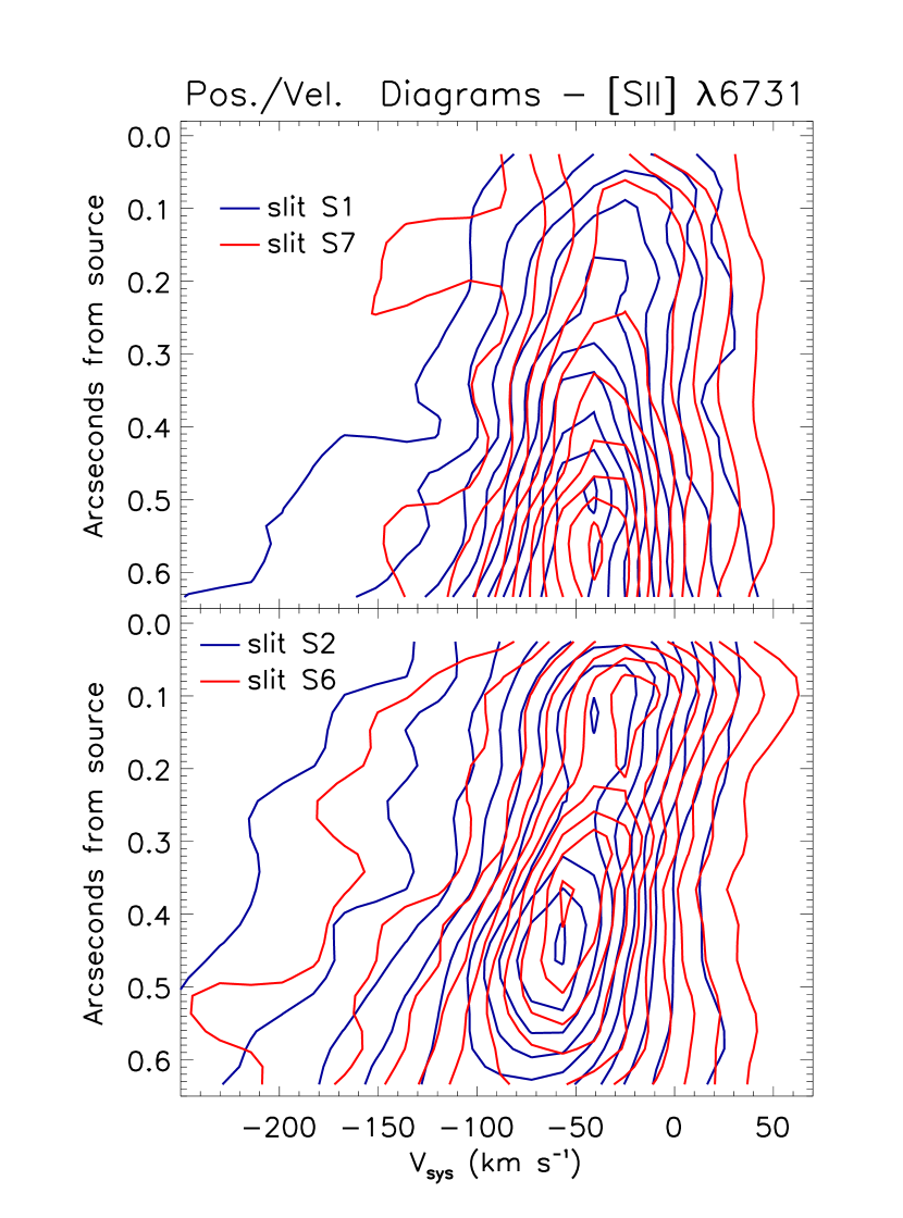
Figure 3: [SII]$\lambda$6731 position-velocity diagrams for the region from 0$\farcs$02 to 0$\farcs$6 from the source. In the top panel contours for equally axially displaced slits S1 (blue) and S7 (red) are compared. The bottom panel shows S2 (blue) and S6 (red). The contour spacing are 10% of the highest contour levels, that correspond to $2.7~{}10^{-14}$, $2.3~{}10^{-14}$, $4.6~{}10^{-14}$ and $3.4~{}10^{-14}$ erg s^-1 cm^-2 Å^-1 arcsec^-2 for S1, S7, S2 and S6 respectively. All velocities are with respect to the systemic velocity of DG Tau, and correction for uneven slit illumination has been applied.

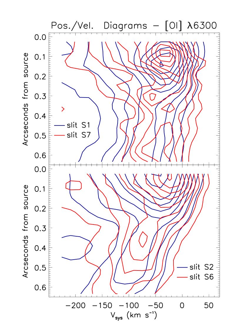
Figure 4: As in Fig. 3 but for the [OI]$\lambda$6300 line. Highest contour levels correspond to $3.3~{}10^{-14}$, $3.3~{}10^{-14}$, $9.0~{}10^{-14}$ and $6.6~{}10^{-14}$ erg s^-1 cm^-2 Å^-1 arcsec^-2 for S1, S7, S2 and S6 respectively.

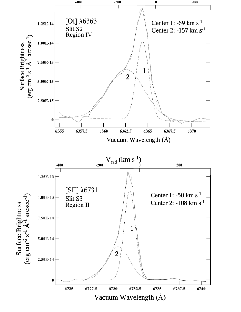
Figure 5: Example of multiple Gaussian fits for the [OI]$\lambda$6363 line in the spectrum from slit S2 and in zone IV (top panel) and for the [SII]$\lambda$6731 line, in zone II and spectrum S3. The analysis presented in the paper is based on the values obtained for the component at low/moderate velocity, labelled with “1” in this Figure

Further illustrations of the lateral global velocity shifts across the flow are shown in Figs.  3 and 4. Fig.  3 contains superimposed position-velocity diagrams for the [SII]$\lambda$6731 line in the region between 0$\farcs$02 to 0$\farcs$6 from the source. In the top panel contours for the slit pair S1 and S7 are compared while the bottom one contrasts S2 and S6. All velocities are with respect to the systemic velocity of DG Tau, and the contour level spacings are in intervals of 10% of each peak value (indicated in the figure captions). The velocity shift between the southeastern and northwestern sides of the flow can be clearly seen. The corresponding diagrams for the [OI]$\lambda$6300 line are displayed in Fig.  4. In Fig.  5 we further show two typical line profiles, which are horizontal cuts of the position-velocity diagrams in selected positions. The Figure also illustrates the adopted multiple Gaussian fit. Our kinematical analysis refer to the well defined low-moderate velocity component labelled with “1” in the figure.

To check whether the observed differential Doppler shifts between the southeastern and northwestern parts of the flow contain any possible systematic effect, we used the same procedures on an emission line that should not produce any apparent differential shift. H$\alpha$, at the stellar position, has three components: an unresolved blueshifted wing at about -230 km s^-1, that probably represents the base of the jet seen in projection, and two other components which are produced at, or very close to, the photosphere. One is at approximately the systemic velocity and the other is a red wing, at about +75 km s^-1, attributed to magnetospheric accretion (Edwards (1997)). As this emission is not resolved spatially in our spectra, it should not show any differential shift even if its formation region is rotating. The result is illustrated in Fig. 6: our analysis shows mean differential velocity shifts of almost zero. This result strongly endorses our claim that the observed differential Doppler shifts in the other lines are not a result of systematic instrumental or illumination effects.

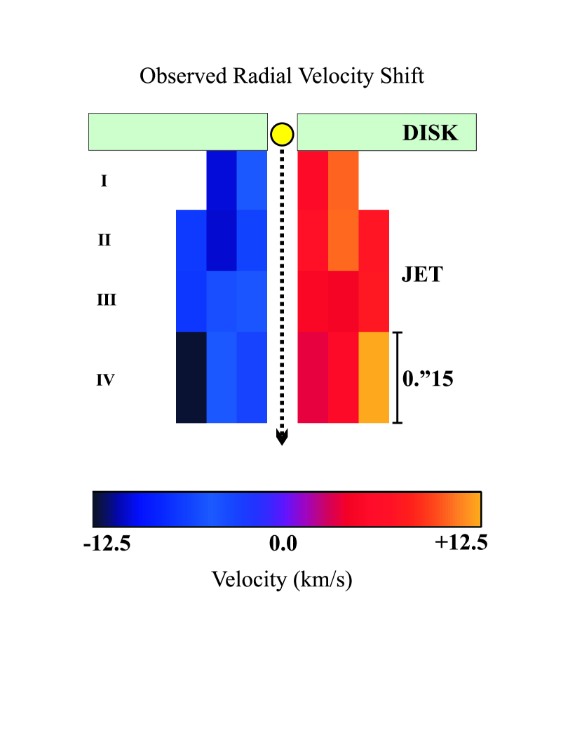
Figure 7: Schematic map of the radial velocity shifts in the southeastern and nortwestern sides of the flow (projected onto the plane of the sky), derived from Table 1. Here the flow is assumed to be axially symmetric. The velocity scale is linear.

If the dectected radial velocity differences are interpreted as rotation, they would imply that the flow is rotating clockwise looking from the tip of the flow toward the source. In Table 1 we list the observed radial velocity shifts, averaged over the values found using the cross-correlation routines (i.e. filled symbols in Fig. 2) for the various lines. In Figure 7, we represent the radial velocity shifts schematically, assuming an axially symmetric flow. Here 0$\farcs$1 corresponds to about 23 AU when de-projected onto the jet meridian plane. Blue and red colors indicate negative and positive projected velocity differences w.r.t. the systemic velocity of the star. The velocity scale is linear. Interpreting the velocity shifts as rotation, and given the inclination angle of the flow, the toroidal velocity of the emitting regions would be between 6 and 15 km s^-1, depending on position. For comparison, the Keplerian velocities in the disk, calculated for M${}_{\star}=0.67$ M_⊙ (Hartigan et al., 1995) are $|7.8|$, $|5.5|$, and $|4.5|$ km s^-1 at 9.8, 19.6 and 29.4 AU from the star, respectively. The latter velocities are given as absolute values, since the sense of rotation of the disk is not yet determined for this star. See further discussion in Sect. 4.

Finally we should emphasise that there are some detailed radial velocity features which cannot be explained by rotation alone. For example, close to the jet, the emission in S7 is faster than S6 but farther out the reverse is true (see Fig. 1). Such discrepancies might well be attributed to clumpiness in the jet, that would be propably revealed with higher angular resolution. In any event it is likely that the jet emission is made up of several overlapping shocks. Also, alternative interpretations to the observed systematic velocity asymmetries could involve non-uniformities in the jet environment, that may cause the bow-shock wings to be angled differently, and/or the jet-ambient entrainment to have different properties on the two sides of the jets. Clearly, studies of more flows are required.

4 Discussion

4.1 Further possible instrumental effects

To test our interpretation of the transverse radial velocity differences in terms of rotation of the flow, we have to exclude other possible causes that could produce such an effect. One source of error might be the orbital motion of the HST, since the linear speed of the spacecraft with respect to the Earth is about 7 km s^-1. Such an effect can however be ruled out, since the exposure time of each spectrum is distributed over the orbital period of the spacecraft. Another way apparent transverse radial velocity differences can be produced is if the sequence of slit positions is not centered on the jet axis. For example let us suppose that the sequence is slightly offset to the northwest. Even if the blueshifted flow from DG Tau is not rotating and perfectly axially symmetric, apparent velocity differences, with the same sign as we observe, would be inferred if the velocity of the flow decreases with increasing distance from the central axis. Such an effect, however, would only be relevant if the misalignment of the slit is about 0.1 arcsec. To determine whether any such offset was present (an unlikely scenario as we had used the STIS ACQ/PEAK option to peak up on the source), we determined the precise position and orientation of the slits by analyzing, with Gaussian fits, transverse intensity profiles in reconstructed images of the initial jet channel. In particular, we used images in the [SII] and [OI] lines (Bacciotti et al., 2000) as well as images of the stellar continuum. Assuming the brightness distribution is axially symmetric, the displacement of the emission peaks with respect to the central slit should indicate the relative position of the latter (and hence, of the system of parallel slits) with respect to the flow axis. The results are displayed in Fig. 8. It turns out that the central slit is (not surprisingly) well positioned on the star, within a small fraction of the slit width, but that the slit orientation is slightly rotated with respect to the flow axis (as defined by the intensity distribution) by about 3°. Note, however, that in the last position (i.e. Region IV) the peak intensity is located on the opposite side of the slit, probably an effect of the opening of the $`$bubble’ (Bacciotti et al., 2000). In any event, such a slight rotation will produce only a marginal asymmetry in velocity (estimated to be below 20% of the detected values). Moreover, if this slight tilt was important, we would expect larger velocity shifts toward the axis of the jet, contrary to what we observe. Thus the small tilt of the slit can neither reproduce the magnitude nor the type of velocity offsets that we detect.

If we are indeed observing rotation of the flow, then it should be in the same sense as in the circumstellar material of the accretion disk and/or the parent molecular cloud. Unfortunately, we do not have any clear indications which way DG Tau’s disk is rotating (A. Sargent, 2001, priv. comm.), while the large-scale molecular environment of the star appears to be characterized by a combination of infall and outflow rather than rotation (Kitamura et al., 1996).

4.2 Comparison with theoretical predictions

A full comparison of the observed velocity values with existing models would require the construction of a simulated spectrum with excitation and kinematic parameters provided by the model. Unfortunately the peripheral regions of the outflow, i.e. the regions we are beginning to resolve, are generally less accurately modeled than the axial portions. That said, we can try to compare our results with general theoretical predictions, assuming that the velocity shifts we observe are indeed due to the presence of rotation. Starting from the seminal work of Blandford and Payne (1982), the popular magneto-centrifugal launching models have been developed by several groups, the most widely known being the the $`$disk wind’ model (see the review by Königl & Pudritz (2000)) and the $`$X-wind’ model, described by Shu et al. (1995, 2000). Similar approaches are also adopted by Camenzind (1997), Ferreira & Pelletier (1995) and Lery et al. (1999). What renders these models particularly attractive is the fact that the outflow extracts angular momentum from the protostar plus disk system, thereby allowing the central object to accrete matter up to its final mass. Without going into the details, we list here a few general properties that are relevant to our study.
(i) The wind is launched along magnetic field lines (in a $`$bead-on-a-wire’ fashion) from a region of the disk between a few stellar radii (X-wind) and a few AU (or more, disk wind). For both cold and warm flows, a wind can be launched if at the footpoint $r_{0}$ the inclination of the magnetic/flow surface with respect to the plane of the disk is less than 60°.
(ii) The surface at which the poloidal velocity, $v_{p}$, equals the characteristic poloidal Alfvèn speed is called the Alfvèn surface (hereafter referred to as the AS). Here, the kinetic fluid energy becomes dominant, and the inertia of the fluid deformes the shape of the field: a strong $B_{\phi}$ component is generated, which tends to collimate the jet (due to hoop stresses). The distance from the axis at which the flow surface intersects the AS is called the Alfvén radius, $r_{A}$. Since the fluid is accelerated up to the AS, the distance $r_{A}-r_{0}$ represents the lever arm of the magnetic field. Up to the AS, the flow slides along the lines of force as if moving with solid body rotation. Hence below the AS $v_{\phi}\propto r$, where $r$ is the radial distance from the rotation axis. Above the AS the flow moves along the magnetic surfaces conserving its angular momentum, and hence here $v_{\phi}\propto r^{-1}$.
(iii) For a $`$cold’ flow (i.e. enthalpy negligible with respect to kinetic and magnetic energy), the terminal poloidal velocity along each magnetic/flow surface is given by $v_{p,\infty}\sim 2^{1/2}(r_{A}/r_{0})v_{K}$, where $v_{K}=(GM_{\star})^{1/2}r^{-1/2}_{0}$ is the Keplerian velocity in the disk at the footpoint.
(iv) If viscous stresses are negligible with respect to the magnetic torque, the concept of global angular momentum conservation finds its formal translation in the simple relationship: $\dot{M}_{\rm jet}/\dot{M}_{\rm acc}\sim(r_{0}/r_{A})^{2},$ where $\dot{M}_{\rm jet}$ and $\dot{M}_{\rm acc}$ are the rates of mass flow within the jet and accreted through the disk, respectively.
(v) The ratio $r_{A}/r_{0}$ varies between the models, but it is generally found to be in the range 2 – 5, both on analytical and numerical grounds. As a consequence, $\dot{M}_{\rm jet}/\dot{M}_{\rm acc}\sim 0.1$, in agreement with observed values for various jets (including the DG Tau outflow itself, see Bacciotti et al. (2002)).

If we now turn to our results, we can first check if the values obtained for the toroidal velocities are in the right range for magneto-centrifugal acceleration. In Bacciotti et al. (2002) we estimate that $\dot{M}_{\rm jet}/\dot{M}_{\rm acc}\sim 0.1$ for this flow. Thus from (iv) and (v) we deduce that on average $r_{A}=3\,r_{0}$. We will assume for simplicity that the same ratio holds for any magnetic/flow surface rooted in the disk. From Fig. 1 we deduce that the average radial velocity measured on the jet symmetry axis for the resolved flow is -70 km s^-1, which de-projected along the flow surfaces gives $v_{p}=$ -80 km s^-1 (see Bacciotti et al. (2002) for details). If we take this value as the terminal velocity $v_{p,\infty}$ of the velocity interval we are looking at, and we assume a cold flow, we deduce from (iii) that $v_{K}\sim$ 18 km s^-1. Hence the launching region for this zone is centered at $r_{0}\sim$ 1.8 AU. Let us now follow the fluid particle (the $`$bead’) in its movement from the footpoint $r_{0}$ along the representative magnetic line (the $`$wire’) rooted at $r_{0}$. According to (ii), matter acquires its maximum linear rotational velocity at the AS, which in the present example crosses the relevant flow surface at $r_{A}\sim 5.4$ AU from the axis (and hence below the resolution limit of HST itself). Here $v_{\phi,max}\sim 54$ km s^-1. After the passage through the AS, the flow starts to lag behind, conserving its angular momentum. The expected value of $v_{\phi}$ at a distance $r$ from the axis depends on model details, and in particular upon the shape of the magnetic surfaces. We can estimate, however, that angular momentum conservation above the AS would yield $v_{\phi}=$ 29, 15 and 10 km s^-1 if the magnetic surface is responsible for the flow at 10, 20 and 30 AU from the axis, respectively. Thus we see that the toroidal velocities we have inferred in Section 3 from our observations for similar distances from the rotation axis (and well above the expected location of the AS) are in very good agreement with the range provided by simple and very general theoretical arguments.

We can take a step further by estimating the angular momentum flux $\dot{J}_{w,lm}$ in the low to moderate velocity region of the flow. This is given by

$$\dot{J}_{w,lm}=\int^{r_{\rm out}}_{r_{\rm in}}\rho~{}v_{p}~{}rv_{\phi}~{}2\pi r~{}dr,$$

where $\rho$ is the total mass density and $r_{\rm in}$ and $r_{\rm out}$ are the inner and outer radii, at a given height above the disk, of the partially hollowed-out cone containing the low to moderate velocity flow. Since the detailed variation of these quantities across the jet are not available from observations, we will make a simplified estimate using mass loss rates and flow radii (for the aforementioned velocity intervals) from Bacciotti et al. (2002). The regime examined, isolated on the basis of the shape of the line profiles, is the combination of the LVI ($v_{\rm rad}=$ +55 to -70 km s^-1) and MVI ($v_{\rm rad}=$ -70 to -195 km s^-1). For these intervals, the mass loss rates are calculated to be 8.3 10^-8 M_⊙ yr^-1 (LVI), and 5.1 10^-8 M_⊙ yr^-1 (MVI). Thus, assuming that in both the LVI and the MVI the average toroidal velocity is $\bar{v}_{\phi}=15$ km s^-1 we can estimate the angular momentum flux as

$$\dot{J}_{w,lm}=\bar{v}_{\phi}(\dot{M}_{\rm LVI}\bar{r}_{\rm LVI}+\dot{M}_{\rm MVI}\bar{r}_{\rm MVI})~{}\sim~{}3.8\,10^{-5}\,{\rm M_{\odot}\,yr^{-1}\,AU\,km\,s^{-1}},$$

where $\bar{r}_{\rm LVI}=$ 21.6 AU and $\bar{r}_{\rm MVI}=$ 14 AU are the average radii of the zones.

For comparison, we calculate the angular momentum loss rate $\dot{J}_{D,r_{0}}$ that the disk must sustain at the footpoint $r_{0}$ in order to let the matter move inward with the observed $\dot{M}_{\rm acc}\approx$ 2 10^-6 M_⊙ yr^-1 (Hartigan et al., 1995; Bacciotti et al., 2002). It turns out that $\dot{J}_{D,r_{0}}\sim$ 6.5 10^-5 M_⊙ yr^-1 AU km s^-1. Thus the flux carried away by the wind in the low to moderate velocity intervals amounts to about 60% of the necessary angular momentum loss for the disk at its footpoint. As we used several simplifying assumptions, the true angular momentum flux carried by the wind could be as much as 100% of that transported by the disk. Note however that viscous stresses could also transfer angular momentum outwards through the disk itself. If such stresses are significant, the simple relationship in (iv) becomes invalid. Also, we note that the above considerations assume steady state conditions. On the other hand, DG Tau is known to be highly variable, and variability obviously introduces further uncertainties.

5 Conclusions

Many features of the collimated HH jets associated with star formation are still unexplained, especially the origin of the jets themselves. Models for the launching of flows still lack observational constraints, due to the small size of the acceleration zone and the fact that the central sources are often heavily embedded. In order to shed some light on this area, we have taken and analysed a set of seven high angular resolution ($\leq 0\farcs 1$) HST/STIS spectra of the outflow from the T Tauri star DG Tau. Here we report possible evidence for rotation in this dataset: rotation, in fact, is a fundamental ingredient for the modelling of the acceleration of outflows and of the interplay between accretion and ejection of matter in the framework of the formation of a new star.

From a detailed analysis of the line profiles in each spectrum, and in four distinct regions of the initial part of the jet (within about 100 AU from the star), we have found systematic differences in the radial velocity of the lines for each pair of slits displaced symmetrically with respect to the jet axis. The values, obtained with multiple Gaussian fitting and/or cross-correlation routines, have been corrected for the wavelength offset produced by the uneven illumination of the STIS slit. Other possible instrumental effects that may contaminate the data are either absent or unimportant. According to our results, and under the assumption that the flow is axially symmetric, the southeastern side of the blueshifted jet appears to move toward the observer faster than the corresponding northwestern side, and the average value found for the difference is about 10 km s^-1. A detailed map of the shifts is available in Fig. 7, derived from the values in Table 1. If we interpret these findings in terms of rotation of the flow, they would imply that the jet is rotating clockwise looking from the flow tip towards the source. Taking into account the inclination of this system with respect to the line of sight, one would derive apparent toroidal velocities of around 6 to 15 km s^-1 at a few tens of AU from the axis, and between 20 to 90 AU above the disk plane. These velocities would be in the range predicted by MHD theories. We also estimate the angular momentum flux in the low to medium velocity regime to be about 3.8 10^-5 M_⊙ yr^-1 AU km s^-1. This could amount to 60% of the angular momentum that the disk has to loose per unit time at the footpoint in order to accrete at the observed rate. Our findings may constitute the first detection of rotation in the initial channel of a jet flow, although at the present stage we cannot exclude that non-uniformities in the jet and/or in its environment cause the observed asymmetries. More observations of this and other outflows are required. If the future studies will confirm the presence of rotational motions at the base of the flows, it would represent an important validation of magneto-centrifugal models for the launching of both galactic and extra-galactic jets.

Appendix A Correction for uneven slit illumination

Following Marconi et al. (2002) the light distribution at a point $(x,y)$ on the focal plane of the telescope can be expressed as $\Phi(x,y,v)=\int\int^{+\infty}_{-\infty}dx^{\prime}dy^{\prime}P(x-x^{\prime},y-y^{\prime})I(x^{\prime},y^{\prime})\phi(v-u(x^{\prime},y^{\prime}))$, where $I$ is the total intensity at a point $(x^{\prime},y^{\prime})$ in a reference frame $X^{\prime},Y^{\prime}$ on the sky, $\phi$ is the intrinsic velocity profile centered at the radial velocity $u(x^{\prime},y^{\prime})$, and $P$ is the instrumental PSF. On the focal plane, the slit is aligned with $Y=Y^{\prime}$, its center is at $(x=x_{0},y=0)$, and its width is $\Delta x$. Past the slit and the spectrograph, the light is recorded on the detector, which combines $x$ and $v$ into the coordinate $w=v+k(x-x_{0})$, interpreted as the measured velocity. In the latter, $k(x-x_{0})$ is the spurious velocity contribution introduced from light entering off the slit center. The coefficient $k$ is given by $k=\Delta w/\Delta\xi$, where $\Delta\xi=0."05477$ is the STIS plate scale in the dispersion direction (Bowers and Baum, 1998) in the considered wavelength range. The expected line profile $\tilde{\Psi}_{i}(w)$ at the pixel row $i$ of the detector is then obtained by integrating the light contributions across the slit and over the width $2\Delta y$ of the $i^{{\rm th}}$ pixel, and by convolving the result with the shape of the pixel in the dispersion direction, a top-hat of width $2\Delta w$. Finally, the average velocity $<v_{i}>$ measured at pixel $i$ along the slit can be expressed through the first order momentum of $\tilde{\Psi}_{i}(w)$ with respect to $w$. More precisely, Marconi et al. (2002) show that

$$<v_{i}>={2\Delta w\int^{x_{0}+\Delta x}_{x_{0}-\Delta x}dx\int^{y_{i}+\Delta y}_{y_{i}-\Delta y}dy\int\int^{+\infty}_{-\infty}dx^{\prime}dy^{\prime}I(x^{\prime},y^{\prime})P(x-x^{\prime},y-y^{\prime})(u+k(x-x_{0}))\over\int^{+\infty}_{-\infty}\tilde{\Psi}_{i}(w)dw}.$$ (A1)

It can thus be argued that if $I$ is not constant across the slit, the term $k(x-x_{0})$ will be weighted differently with varying $x$, and this can cause a spurious velocity offset to appear at the detector. For a point source, and for the adopted STIS configuration, the spurious shift can be up to about 25 km s^-1. The effect is reduced, but not eliminated, if the observed source is extended, as in our case. We estimated the wavelength offsets using numerical routines recently developed by A. Marconi (Marconi et al., 2002). For a given slit width and slit position with respect to the source, the routines calculate the average velocity measured at the detector through Eq. A1, starting from a model intensity and velocity field $I(x^{\prime},y^{\prime}),~{}u(x^{\prime},y^{\prime})$. The adopted PSF is the one generated by TinyTim at 6700 Å, and convolution is done using a Fast Fourier Transform algorithm. To estimate the spurious offset in each line/position, we used a model intensity distribution derived by combining the surface brightness in the LVI and MVI intervals shown in Bacciotti et al. (2000). For the purpose of the calculation, we have then assumed a constant (arbitrary) velocity field $u(x^{\prime},y^{\prime})=\bar{u}$. The difference $(<v_{j}>-\bar{u})$ is thus the value of the instrumental offset to be determined. It should be noted that in the real case in which the velocity field is not constant, the passage through the telescope and spectrograph introduces an additional deformation to the transverse profile of the velocity. In our case, however, this effect should not lead to spurious velocity asymmetries with respect to the central axis, because the radial velocity, as well as the intensity, is increasing (in absolute value) toward the axis on both sides of the jet (see Fig. 1).

Figure 1: Radial velocity values of the line peak at low/moderate velocity, for all slits across the jet (S1 to S7, from the southeastern to the northwestern border of the jet respectively), and in four distinct regions along the flow (I, II, III and IV, see figure for distances from the source). The values are derived from multiple Gaussian fitting of the line profiles, and are corrected for the effects of uneven slit illumination. The error bar illustrates the typical accuracy of the Gaussian fit combined with the one of the STIS pipeline calibration.

Figure 2: Radial velocity differences between slit positions displaced symmetrically with respect to the central slit. Units are km s^-1. Open symbols: difference of the values displayed in Fig. 1 (error bar labeled with ‘gss’). Filled symbols: higher accuracy values obtained by cross-correlating the associated line profiles (error bar label: ‘crc’). In almost all positions the velocity difference is negative, indicating a net relative motion of the southeastern side of the flow with respect to its northwestern side.

Figure 6: Velocity shifts, as in Fig. 2, but for the H$\alpha$ line at the stellar position. The systemic (diamonds), redshifted (triangles) and blueshifted (squares) components of this line have been analysed. All the components are unresolved, and are not expected to show any shift when corrected for the STIS offset. Note that the observed shift is very limited illustrating the high sensitivity of our technique.

Figure 8: Estimate of the spatial displacement of the intensity peak (for the LVI) with respect to the position of the central slit S4 (dotted line). See text for details.

Table 1: Observed radial velocity shifts

Region	$d_{s}$	$d_{j}$	$v_{\rm rad}$ shift for (S1–S7)	$v_{\rm rad}$ shift for (S2–S6)	$v_{\rm rad}$ shift for (S3–S5)
	(″)	(AU)	(km s-1)	(km s-1)	(km s-1)
I	0.075	17	+3.4	-15.8	-8.0
II	0.175	40	-11.0	-16.2	-9.9
III	0.275	62	-11.2	-6.5	-7.2
IV	0.4	91	-19.1	-8.0	-5.1

References

- Bacciotti et al. (2000) Bacciotti, F., Mundt, R., Ray, T.P., Eislöffel, J., Solf, J., & Camezind, M. 2000, ApJ, 537, 49
- Bacciotti et al. (2002) Bacciotti, F., Ray, T.P., Mundt, R., Eislöffel, J., & Solf, J. 2002, in preparation
- Blandford and Payne (1982) Blandford, R. D. and Payne, D.G., 1982, MNRAS, 199 883
- Bowers and Baum (1998) Bowers, C., Baum, S., 1998, STIS Instrumental Report 98-23
- Camenzind (1997) Camenzind, M. 1997, in Herbig-Haro Flows and the Birth of Low Mass Stars, IAU Symp. 182, eds. B. Reipurth and C. Bertout (Kluwer Academic Publishers), 241
- Davis et al. (2000) Davis, C.J., Berndsen, A., Smith, M.D., Chrysostomou, A., & Hobson, J. 2000, MNRAS, 314, 241
- Edwards (1997) Edwards, S. 1997, in Herbig-Haro Flows and the Birth of Low Mass Stars, IAU Symp. 182, eds. B. Reipurth and C. Bertout (Kluwer Academic Publishers), 433
- Eislöffel & Mundt (1998) Eislöffel, J., & Mundt, R. 1998, AJ, 115, 1554
- Eislöffel et al. (2000) Eislöffel, J., Mundt, R., Ray, T.P., & Rodríguez, L.F. 2000, in ‘Protostars and Planets IV’ , Tucson: University of Arizona Press; eds Mannings, V., Boss, A.P., Russell, S.S., 815
- Ferreira & Pelletier (1995) Ferreira, J., & Pelletier, G. 1995, A&A, 295, 8
- Hartigan et al. (1995) Hartigan P., Edwards S., & Gandhour L. 1995, ApJ, 452, 736
- Kitamura et al. (1996) Kitamura, Y., Kawabe, R., & Saito, M. 1996, ApJ, 457, 277
- Königl & Pudritz (2000) Königl, A., & Pudritz, R.E. 2000, in ‘Protostars and Planets IV’ , Tucson: University of Arizona Press; eds Mannings, V., Boss, A.P., Russell, S.S., p. 759
- Lery et al. (1999) Lery T., Henriksen R.N., & Fiege J.D. 1999, A&A, 350, 254
- Marconi et al. (2002) Marconi, A. et al., 2002, in preparation
- Ray (1998) Ray, T.P., 1998, in Astrophysical Jets: Open Problems, eds. S. Massaglia and G. Bodo, Amsterdam, Gordon & Breach Science Publishers, 173
- Shu et al. (1995) Shu, F.H., Najita, J.R., Ostriker, E., & Shang, H. 1995, ApJ, 455, L155
- Shu et al. (2000) Shu, F.H., Najita, J.R., Shang, H., & Li, Z.-Y., in ‘Protostars and Planets IV’, Tucson: University of Arizona Press; eds Mannings, V., Boss, A.P., Russell, S.S., 789
- Shibata & Kudoh (1999) Shibata, K., & Kudoh, T. in Proceedings of ”Star Formation 1999”, held in Nagoya, Japan, June 21 - 25, 1999, Editor: T. Nakamoto, Nobeyama Radio Observatory, p. 263-268