Gravitational Microlensing Near Caustics II: Cusps

Abstract

We present a rigorous, detailed study of the generic, quantitative properties of gravitational lensing near cusp catastrophes. Concentrating on the case when the individual images are unresolved, we derive explicit formulas for the total magnification and centroid of the images created for sources outside, on, and inside the cusped caustic. We obtain new results on how the image magnifications scale with respect to separation from the cusped caustic for arbitrary source positions. Along the axis of symmetry of the cusp, the total magnification $\mu$ scales as $\mu\propto u^{-1}$, where $u$ is the distance of the source from the cusp, whereas perpendicular to this axis, $\mu\propto u^{-2/3}$. When the source passes through a point $\mbox{\boldmath$u$}_{0}$ on a fold arc abutting the cusp, the image centroid has a jump discontinuity; we present a formula for the size of the jump in terms of the local derivatives of the lens potential and show that the magnitude of the jump scales as $|u^{0}_{1}|^{1/2}$ for $|u^{0}_{1}|\ll 1$, where $|u^{0}_{1}|$ is the horizontal distance between $\mbox{\boldmath$u$}_{0}$ and the cusp. The total magnifications for a small extended source located both on, and perpendicular to, the axis of symmetry are also derived, for both uniform and limb darkened surface brightness profiles. We find that the difference in magnification between a finite and point source is $\lesssim 5\%$ for separations of $\gtrsim 2.5$ source radii from the cusp point, while the effect of limb-darkening is $\lesssim 1\%$ in the same range. Our predictions for the astrometric and photometric behavior of both pointlike and finite sources passing near a cusp are illustrated and verified using numerical simulations of the cusp-crossing Galactic binary-lens event MACHO-1997-BUL-28. Our results can be applied to any microlensing system with cusp caustics, including Galactic binary lenses and quasar microlensing; we discuss several possible applications of our results to these topics.

1 Introduction

Over the past twenty years, gravitational lensing has grown from a mere curiosity to an important component of a large and diverse set of fields in astronomy. Its ubiquity is due at least in part to the fact that its effects are observable over a wide range of scales. This has enabled astronomers to use lensing to study everything from the smallest compact objects, to the largest structures in the universe, and almost everything in between. Despite the diversity of applications of gravitational lensing, the mathematical description of the phenomenon itself is both relatively tractable, and universal. In almost all cases, gravitational lensing can be described by a two-dimensional mapping from a lens plane to light source plane. Once this mapping is specified, all of the properties of a gravitational lens can be derived in principle. The observable properties of lensing, however, depend on the phenomenon to which it is applied. Therefore, lensing is traditionally divided into an number of different regimes, which are delimited by the observables. For example, the term microlensing is typically applied to the case when multiple images occur, but are not resolved. When multiple images are created by a gravitational lens, the separation between these images is typically of order the Einstein ring radius,

$$\theta_{\rm E}=\sqrt{{{4GM}\over c^{2}D}},$$ (1)

where $M$ is the mass of the lens, $D\equiv D_{os}D_{ol}/D_{ls}$, and $D_{os}$, $D_{ol}$, and $D_{ls}$ are the distances from observer to source, observer to lens, and lens to source, respectively. Thus, the term microlensing is applied when $\theta_{\rm E}$ is less than the resolution. In this case, all one can measure is the collective behavior of all the images created by the lens, i.e., the total magnification, and the position of the center-of-light (centroid) of the image. In fact, if the observer, source, and lens were not in relative motion, than the individual image magnifications and positions would be fixed, and even these properties would not be measurable. The relative positions of the observer, lens, and source, and thus the magnification and centroid, are expected to vary on time scales of order the Einstein ring crossing time,

$$t_{\rm E}={\theta_{\rm E}D_{ol}\over v_{\perp}},$$ (2)

where $v_{\perp}$ is the transverse speed of the lens relative to the observer-source line-of-sight. Fortunately, in the two regimes where microlensing has been discussed, the typical values of $\theta_{\rm E}$, $D_{ol}$, and $v_{\perp}$ result in reasonable time scales. Typical values for the lens mass $M$, relative source-lens distance $D$, transverse velocity $v_{\perp}$, and the resulting typical values for $\theta_{\rm E}$ and $t_{\rm E}$ for both Local Group and cosmological microlensing are given in Table 1. Also shown are typical values for the radius $\theta_{*}$ of the source’s emission region, this radius in units of $\theta_{\rm E}$, $\rho_{*}\equiv\theta_{*}/\theta_{\rm E}$, and the time it takes the lens to cross the source, $t_{*}\equiv\rho_{*}t_{\rm E}$. These latter parameters will be relevant to the discussion of finite source effects in §2.4. For the Local Group, a typical Einstein radius crossing time is $t_{\rm E}={\cal O}(100~{}{\rm days})$, whereas for cosmological microlensing, $t_{\rm E}={\cal O}(10~{}{\rm years})$.

	$M$	$D$	$\theta_{\rm E}$	$v_{\perp}$	$t_{\rm E}$	$\theta_{*}$	$\rho_{*}$	$t_{*}$
Local Group	$1M_{\odot}$	$10~{}{\rm kpc}$	$1{\rm mas}$	$100~{}{\rm km~{}s^{-1}}$	$100~{}{\rm days}$	$1\mu{\rm as}$	$10^{-3}$	$0.1~{}{\rm days}$
Cosmological	$1M_{\odot}$	$1~{}{\rm Gpc}$	$3\mu{\rm as}$	$500~{}{\rm km~{}s^{-1}}$	$10~{}{\rm years}$	$0.1\mu{\rm as}$	$0.03$	$100~{}{\rm days}$

Table 1 Typical Microlensing Parameters.

Of exceptional importance in microlensing is the existence of caustics: positions in the light source plane corresponding to the critical values of the lens mapping. On caustics, at least one image is formed that has formally infinite magnification (for a point-source). When a source crosses a caustic, both the total magnification and centroid of all the images exhibit instantaneous, discontinuous jumps. These jumps are averaged out over the finite source size; however, it is generically true that large gradients in the magnification and centroid exist near caustics. Furthermore, microlensing caustics have several important and useful properties. First, the large magnification results in a large photon flux from the source. Second, the large gradient in the magnification and centroid with respect to source position effectively implies high angular resolution. Finally, the highly localized nature of the high-magnification and large centroid-shift regions created by caustics results in characteristic, and easily-recognizable features, in both astrometric and photometric microlensing curves. Many authors have suggested exploiting these properties of caustics to study a number of astrophysical applications, i.e., stellar multiplicity (Mao & Paczyński, 1991), stellar atmospheres (Gould, 2001), individual microlens mass measurements (Graff & Gould, 2002), microlens mass functions (Wyithe, Webster, & Turner, 2000), properties of the emission regions of quasars (Wambsganss, Paczynski, & Schneider, 1990; Agol & Krolik, 1999; Fluke & Webster, 1999; Wyithe, Webster, & Turner, 2000), and lens transverse velocities (Wyithe, Webster, & Turner, 1999). See Gaudi & Petters (2002; hereafter Paper I) for a more thorough discussion of the uses of astrometric and photometric microlensing observations in the presence of caustics in both Local Group and cosmological contexts.

Although the caustic curves of gravitational lenses exhibit an enormously rich and diverse range of properties, it can be shown rigorously that each stable lensing map has only two types of caustic singularities: folds and cusps (Petters, Levine, & Wambsganss 2001, p. 294). Each of these two types of singularities have generic and universal properties and, in particular, each can be described by a polynomial mapping from the lens plane to light source plane. The coefficients of these mappings depend on local derivatives of the dimensionless surface potential of the lens. In Paper I, we used the mapping for a fold singularity to derive the observable properties of gravitational lensing near folds, paying particular attention to the case of microlensing, in which the images are unresolved. We derived analytic expressions for the total magnification and centroid shift near a generic, parabolic, fold caustic. We then showed how these expressions reduce to those for the more familiar linear fold, which lenses a nearby source into two equal magnification, opposite parity images whose total magnification is proportional to $u^{-1/2}$, where $u$ is the distance of the source to the fold caustic. We then generalized these results to finite source sizes. Finally, we compared our analytic results to numerical simulations of the Galactic binary-lens event OGLE-1999-BUL-23, in which the source was observed to cross a fold caustic. We found excellent qualitative agreement between our analytic and semi-analytic expressions for the photometric and astrometric behavior near a fold caustic, and our detailed numerical simulations of the second fold caustic crossing of OGLE-1998-BUL-23.

In this paper, we present a similarly detailed study of the generic, quantitative properties of microlensing near cusps. Although fold caustic crossings are expected and observed to dominate the sample of caustic crossings in Galactic binary events (Gaudi & Gould, 1999; Gaudi, Graff, & Han, 2002; Alcock et al., 2000), cusp crossings will nevertheless represent a non-negligible fraction of all caustic crossing events. In fact, at least two cusp crossing events have already been observed, the Galactic bulge events MACHO 97-BLG-28 (Albrow et al., 1999a), and MACHO-1997-BLG-41 (Alcock et al., 2000; Albrow et al., 2000). It is interesting to note that the analyses and modeling of these events were performed using entirely numerical methods. As we discuss in some detail (see §5), we believe that the analytic results derived here are particularly amenable to the analysis of MACHO 97-BLG-28  and similar events. In the cosmological context, the role of cusps versus folds is less clear, due primarily to the more complicated structure of the caustics themselves. However, it has been shown that, in the limit of high magnifications, the inclusion of cusps alters the form of the total microimage magnification cross section, due to the lobe of high-magnification close to and outside the cusped caustic (Schneider & Weiss, 1992). Lensing near cusps has been substantially less well-studied than lensing near folds, and as a result, useful analytic expressions for the observable properties are few. Previous studies have focused almost exclusively on the magnification of the images created by a cusp singularity (Schneider & Weiss, 1992; Mao, 1992; Zakharov, 1995, 1999). Here we study all the observable properties of gravitational microlensing near cusps, including the photometric (total magnification) and astrometric (light centroid) behavior, for both point sources and extended sources with arbitrary surface brightness profiles.

The layout of this paper is as follows. In §2, we derive analytic expressions for the image positions, magnification, and light centroid for sources near a generic cusp. In §2.1 we define the observable microlensing properties. In §2.2, we start with the generic expression for the mapping near a cusp, and derive all the properties for the local images for sources exterior to (§2.2.2), on (§2.2.3), and interior to (§2.2.4) the caustic. We generalize the discussion to include images not associated with the cusp in §2.3, and study extended sources in §2.4. In §3, we illustrate the observable behavior near a cusp by numerically simulating the Galactic binary-lens cusp-crossing event MACHO 97-BLG-28, and directly compare these numerical results with our analytic expressions in §4. In §5, we suggest several possible applications in both local group and cosmological contexts. We summarize and conclude in §6. We note that, for the sake of completeness, we include some results that have been presented elsewhere. Combined with the results from Paper I, the results presented here describe the observable properties of gravitational microlensing near all stable singularities.

2 Analytical Treatment

2.1 General Equations for Magnification and Image Centroid

The lens equation due to a gravitational lens with potential $\psi$ is given in dimensionless form as follows:

$$\mbox{\boldmath$u$}=\mbox{\boldmath$\theta$}-{\mbox{\boldmath$\alpha$}}(\mbox{\boldmath$\theta$}).$$ (3)

Here $\mbox{\boldmath$\theta$}={\bf r}/(\theta_{\rm E}D_{ol})$ and $\mbox{\boldmath$u$}={\bf s}/({\theta_{\rm E}D_{os}})$, where $r$ and $s$ denote the proper vector positions in the lens and light source planes, respectively, and ${\mbox{\boldmath$\alpha$}}(\mbox{\boldmath$\theta$})\equiv{\mbox{\boldmath$\nabla$}}\psi(\mbox{\boldmath$\theta$}).$ Note that if $\kappa$ is the surface mass density of the lens in units of the critical density $\Sigma_{cr}\equiv(c^{2}D_{os})/(4\pi GD_{ol}D_{ls})$, then the gravitational lens potential $\psi$ is related to $\kappa$ by

$$\psi(\mbox{\boldmath$\theta$})=\frac{1}{\pi}\int_{\rm R^{2}}d{\mbox{\boldmath$\theta$}^{\prime}}\kappa(\mbox{\boldmath$\theta$}^{\prime})\ln|\mbox{\boldmath$\theta$}-\mbox{\boldmath$\theta$}^{\prime}|.$$ (4)

The lens equation induces a lensing map $\eta$ from the lens plane $L$ into the light source plane $S$ defined by ${\mbox{\boldmath$\eta$}}(\mbox{\boldmath$\theta$})=\mbox{\boldmath$\theta$}-{\mbox{\boldmath$\alpha$}}(\mbox{\boldmath$\theta$})$. The critical curves of $\eta$ are defined to be the locus of all critical points of $\eta$, i.e., the set of solutions $\mbox{\boldmath$\theta$}_{c}$ of the equation

$$\mathop{\rm det}\nolimits[A_{\mbox{\boldmath$\eta$}}](\mbox{\boldmath$\theta$}_{c})=0,$$ (5)

where $A_{\mbox{\boldmath$\eta$}}$ is the Jacobian matrix of $\eta$. The caustics of $\eta$ are its critical values, i.e., the set of all points $\mbox{\boldmath$u$}_{c}={\mbox{\boldmath$\eta$}}(\mbox{\boldmath$\theta$}_{c})$.

For a fixed source position $u$, the solutions in $L$ of the lens equation determine the lensed images of $u$. Suppose that a source at $u$ has $N(\mbox{\boldmath$u$})$ images. The magnification of the $i$th image $\mbox{\boldmath$\theta$}_{i}=\mbox{\boldmath$\theta$}_{i}(\mbox{\boldmath$u$})$ is given by

$$\mu(\mbox{\boldmath$\theta$}_{i})=\frac{1}{|\mathop{\rm det}\nolimits[A_{\mbox{\boldmath$\eta$}}](\mbox{\boldmath$\theta$}_{i})|}.$$ (6)

Then the total magnification is

$$\mu_{\rm tot}(\mbox{\boldmath$u$})=\displaystyle\mathop{\sum}_{i=1}^{N(\mbox{\boldmath$u$})}\mu(\mbox{\boldmath$\theta$}_{i}).$$ (7)

For a source at $u$, the image centroid or center-of-light, denoted by ${\mbox{\boldmath$\theta$}}_{\rm cl}(\mbox{\boldmath$u$})$, and shifted image centroid, which is denoted by $\delta{\mbox{\boldmath$\theta$}}_{\rm cl}$, are defined respectively as follows:

$${\mbox{\boldmath$\theta$}}_{\rm cl}(\mbox{\boldmath$u$})=\frac{1}{\mu_{\rm tot}(\mbox{\boldmath$u$})}\displaystyle\mathop{\sum}_{i=1}^{N(\mbox{\boldmath$u$})}\mu(\mbox{\boldmath$\theta$}_{i})\mbox{\boldmath$\theta$}_{i},\hskip 36.135pt\delta{\mbox{\boldmath$\theta$}}_{\rm cl}(\mbox{\boldmath$u$})={\mbox{\boldmath$\theta$}}_{\rm cl}(\mbox{\boldmath$u$})-\mbox{\boldmath$u$}.$$ (8)

The image centroid is defined analogously to a center of mass. However, the image centroid is much more complicated since images can suddenly be created or annihilated as the source moves over caustics. For the case of gravitational microlensing, the total magnification and shifted centroid are observables, with the latter expected to be accessible to, e.g. the Space Interferometry Mission (SIM).

2.2 Local Case: Point Sources Near a Cusp

A rigorous analytical study of the total magnification (photometry) and image centroids (astrometry) for most physically reasonable lens models (e.g., binary point mass lenses) is very difficult. Our goal here, as in Paper I, is to study the local, generic behavior of these observables near an arbitrary, but fixed, critical point of a given type. In Paper I, we studied the behavior near a fold singularity; here we study the behavior near a cusp. In order to study the local behavior near singularities, we Taylor expand the scalar potential $\psi$ in the neighborhood of the singularity, keeping terms to a specified order in the image position $\theta$. We note that the order at which one chooses to truncate the expansion is somewhat arbitrary; higher accuracy can always be achieved by keeping terms of higher order (at the expense of higher complexity, of course). However, it is generically true that fold critical points are characterized by partial derivatives of the lensing map up to second order, while cusps are classified by partials up to third order (Petters et al. 2001, pp. 370-371). As a result, the Taylor expansion of the potential is usually taken up to second order for the fold and third order for the cusp. See Schneider et al. (1992, pp. 187-188) and particularly Petters et al. (2001, pp. 341-353) for more discussion on truncation of Taylor expansions of the potential. After introducing an orthogonal change in coordinates, one can thus obtain a simpler equation that approximates the quantitative, generic behavior of the total magnification and image centroid of sources near a critical point. Consider a generic lensing map $\eta$ whose caustics have cusps. In such a case, there are at least two cusps since the total number of cusps is always even (see Petters 1995, p. 4282, for a cusp-counting formula). In this section we will fix one of the cusps and study the behavior of $\eta$ in the vicinity of that cusp.

2.2.1 Local Case: Magnification and Centroid of Images Associated with the Cusp

Without loss of generality, we can assume that the coordinates $\theta$ on the lens plane $L$ and $u$ on the light source plane $S$ are translated so that the cusp lies at the origin ${\bf 0}$ of $S$ and ${\mbox{\boldmath$\eta$}}({\bf 0})={\bf 0}$. There is an orthogonal change of the coordinates $\theta$ and $u$ which is the same in the lens and light source planes such that the lensing map $\eta$ can be approximated by the following simpler mapping in a neighborhood of the origin (Petters et al. 2001, pp. 341-353; Schneider et al. 1992, p. 193):

$$u_{1}=c\theta_{1}+\frac{b}{2}\theta^{2}_{2},\qquad u_{2}=b\theta_{1}\theta_{2}+a\theta_{2}^{3},$$ (9)

where

$$a=-\frac{1}{6}\psi_{2222}({\bf 0}),\quad b=-\psi_{122}({\bf 0})\neq 0,\quad c=1-\psi_{11}({\bf 0})\neq 0,\quad 2ac-b^{2}\neq 0.$$ (10)

Note that in (9) we are abusing notation somewhat by using the notation $\mbox{\boldmath$\theta$}=(\theta_{1},\theta_{2})$ and $\mbox{\boldmath$u$}=(u_{1},u_{2})$ for the global lens equation (3) to express the local lens equation. For the explicit relationship between the local coordinates in equation (9) and the global ones in equation (3), see pp. 344-345 of Petters et al. (2001). It is also important to add that the partials in (10) are with respect to the original global coordinates of the lens equation. Figure 1 illustrates the coordinate systems and basic properties of lensing near a cusp. For this figure, we have adopted the coefficients $a=1.69,b=2.45$, and $c=2.0$. These are the appropriate values for the cusp in the observed event MACHO 97-BLG-28. See §4.

We shall now use the lens mapping determined by equation (9) to study the approximate behavior of the magnification and image centroid near a cusped caustic curve. The magnification matrix $A$ for the cusp is the Jacobian matrix of equation (9),

$$A=\left(\begin{array}[]{lc}c&b\theta_{2}\\ b\theta_{2}&b\theta_{1}+3a\theta_{2}^{2}\end{array}\right),$$ (11)

which has the determinant

$$\mathop{\rm det}\nolimits A=bc\theta_{1}+(3ac-b^{2})\theta_{2}^{2}.$$ (12)

The cusp critical point of the mapping in equation (9) is at the origin of the lens plane and mapped to a cusp caustic point at the origin of the light source plane. By equation (12), the critical curve is a parabola,

$$\theta_{1}=\frac{b^{2}-3ac}{bc}\theta_{2}^{2}.$$ (13)

Equations (9) and (13) yield that points $\mbox{\boldmath$u$}_{c}=(u_{c,1},u_{c,2})$ on the caustic are given by

$$u_{c,1}=\frac{3(b^{2}-2ac)}{2b}\theta_{2}^{2},\qquad u_{c,2}=\frac{b^{2}-2ac}{c}\theta_{2}^{3},$$ (14)

where $\theta_{2}$ acts as a parameter along the caustic. The magnitude of the curvature of the caustic is

$$|k|=\frac{|u_{c,1}^{\prime}\ u_{c,2}^{\prime\prime}-u_{c,2}^{\prime}\ u_{c,1}^{\prime\prime}|}{[(u_{c,1}^{\prime})^{2}+(u_{c,2}^{\prime})^{2}]^{3/2}}=\frac{|b\ c|}{3(b^{2}+c^{2})\ |b^{2}-2ac|}\ \frac{1}{|\theta_{2}|},$$

where the primes indicate differentiation with respect to $\theta_{2}$. The curvature diverges as the cusp is approached ($\theta_{2}\rightarrow 0$).

By equation (14), the caustic can also be described as the level curve

$$C(\mbox{\boldmath$u$})\equiv\frac{8b^{3}}{27c^{2}(2ac-b^{2})}u_{1}^{3}+u_{2}^{2}=0.$$ (15)

The origin is a positive cusp if $2ac>b^{2}$ and a negative cusp if $2ac<b^{2}$. Without loss of generality, we shall assume that the cusp is positive. For this case, both $a$ and $c$ have the same sign. The conditions $C(\mbox{\boldmath$u$})>0$, $C(\mbox{\boldmath$u$})=0$, and $C(\mbox{\boldmath$u$})<0$ determine points $u$ outside, on, and inside the cusped caustic curve, respectively.

Let us determine the local lensed images and their magnifications for sources near the cusped caustic. The expression for $u_{1}$ in equation (9) yields

$$\theta_{1}=\frac{u_{1}}{c}-\frac{b}{2c}\theta_{2}^{2}.$$ (16)

Plugging equation (16) into the expression for $u_{2}$ in equation (9), we obtain a cubic equation for $\theta_{2}$ in terms of the source position $(u_{1},u_{2})$:

$$f(\theta_{2})\equiv\theta_{2}^{3}+{\rm p}\ \theta_{2}+{\rm q}=0,$$ (17)

where

$${\rm p}={\rm p}(u_{1})=\frac{2b}{2ac-b^{2}}u_{1},\qquad{\rm q}={\rm q}(u_{2})=-\frac{2c}{2ac-b^{2}}u_{2}.$$ (18)

In other words, the lensed images are points $\mbox{\boldmath$\theta$}=(\theta_{1},\theta_{2})$ with $\theta_{1}$ given by equation (16) and $\theta_{2}$ a real root of equation (17). The magnification of each lensed image $\theta$ of $u$ is then

$$\mu(\mbox{\boldmath$\theta$})=\frac{1}{|\mathop{\rm det}\nolimits A|},$$ (19)

where

$$\mathop{\rm det}\nolimits A=bu_{1}+\frac{3}{2}(2ac-b^{2})\theta_{2}^{2}$$ (20)

with $\theta_{2}$ a real zero of $f$.

For a source at angular vector position $u$, let $\mbox{\boldmath$\theta$}_{*}(\mbox{\boldmath$u$})=(\theta^{*}_{1}(\mbox{\boldmath$u$}),\theta^{*}_{2}(\mbox{\boldmath$u$}))$ be any lensed image of $u$ associated with the cusp, i.e.,

$$\mbox{\boldmath$\theta$}_{*}(\mbox{\boldmath$u$})=\left(\frac{u_{1}}{c}-\frac{b}{2c}[\theta^{*}_{2}(\mbox{\boldmath$u$})]^{2},\theta^{*}_{2}(\mbox{\boldmath$u$})\right),$$ (21)

where $\theta^{*}_{2}(\mbox{\boldmath$u$})$ is a solution of cubic equation (17). Then equation (14) yields that

$$u^{*}_{c,1}=\frac{3(b^{2}-2ac)}{2b}(\theta^{*}_{2})^{2},\qquad u^{*}_{c,2}=\frac{b^{2}-2ac}{c}(\theta^{*}_{2})^{3},$$ (22)

is a point on the caustic. It is important to note that even for a source position $\mbox{\boldmath$u$}=\mbox{\boldmath$u$}_{c}$ at a caustic point, there is no guarantee that the caustic point $\mbox{\boldmath$u$}^{*}_{c}=(u_{c,1}^{*},u_{c,2}^{*})$ equals $\mbox{\boldmath$u$}_{c}$ (see Eq.[53] below). Now, consider the tangent line to the cusp, which happens to coincide with the $u_{1}$-axis (due to our coordinate choice). We shall also refer to this tangent line as the axis of the cusp, since it coincides with the axis of symmetry of the cusp. Note that by (11) the magnification matrix $A({\bf 0})$ at the origin, maps the entire lens plane into the previous tangent line. Define the horizontal distance between $\mbox{\boldmath$u$}=(u_{1},u_{2})$ and $\mbox{\boldmath$u$}^{*}_{c}=(u^{*}_{c,1},u^{*}_{c,2})$ to be the distance between $u$ and $\mbox{\boldmath$u$}^{*}_{c}$ along the direction parallel to the tangent line to the cusp. Denoting the horizontal distance by $\Delta u^{*}_{1,\vdash}$, we obtain

$$\Delta u^{*}_{1,\vdash}\equiv|u_{1}-u^{*}_{c,1}|=|u_{1}-\frac{3(b^{2}-2ac)}{2b}(\theta^{*}_{2})^{2}|.$$ (23)

By equation (20), we see that the magnification of $\mbox{\boldmath$\theta$}_{*}$ is inversely proportional to the horizontal distance between $u$ and $\mbox{\boldmath$u$}^{*}_{c}$:

$$\mu(\mbox{\boldmath$\theta$}_{*})=\frac{1}{|b|\Delta u^{*}_{1,\vdash}}.$$ (24)

We shall see that if the source is on the $u_{1}$-axis, then the magnification of the image $\mbox{\boldmath$\theta$}_{*}$ (only one image occurs locally for sources outside the caustic) is proportional to $u^{-1}$, where $u$ is the distance between the source and cusp (see Eqs.[36] and [70] below). If the source is on the $u_{2}$-axis, then the magnification of $\mbox{\boldmath$\theta$}_{*}$ (again, only one image occurs locally) is proportional to $u^{-2/3}$ (see Eqs. 33). In both cases, the horizontal distance coincides with the ordinary distance.

We note that in Paper I, we showed that the magnification of an image $\mbox{\boldmath$\theta$}_{*}$ associated with the fold caustic is inversely proportional to the square root of the perpendicular distance of the source from the fold. For a generic local fold lensing map that maps a fold critical point at the origin to a fold caustic point at the origin, the perpendicular distance is defined relative to the direction perpendicular to the tangent line to the fold caustic at the origin. Note that the magnification matrix $A({\bf 0})$ for the fold also maps the entire lens plane into the tangent line.

Now, the reals zeros of the polynomial $f$ in equation (17) are characterized using the discriminant of $f$, i.e.,

$$D(\mbox{\boldmath$u$})\equiv\left(\frac{{\rm p}}{3}\right)^{3}+\left(\frac{{\rm q}}{2}\right)^{2}=\frac{c^{2}}{(2ac-b^{2})^{2}}C(\mbox{\boldmath$u$}).$$ (25)

By equation (25), the conditions $D(\mbox{\boldmath$u$})>0$, $D(\mbox{\boldmath$u$})=0$, and $D(\mbox{\boldmath$u$})<0$ also determine, respectively, points $u$ outside, on, and inside the cusped caustic curve. It will be seen that for a source outside, on, or inside the cusped caustic, there are locally one, two, or three images, respectively. These images lie in the neighborhood of the origin, which is a point on the critical curve. The magnification and centroid of the images associated with the cusp will be denoted by $\mu_{\rm loc}$ and ${\mbox{\boldmath$\theta$}}_{\rm loc}$, respectively., and called the local magnification and local image centroid. We shall now determine $\mu_{\rm loc}$ and ${\mbox{\boldmath$\theta$}}_{\rm loc}$ for source positions near the cusp that are outside, on, and inside the caustic — see equations (80) and (81) for a summary.

2.2.2 Local Case: Source Outside the Cusp

For a source position $u$ outside and near the cusp (i.e., $D(\mbox{\boldmath$u$})>0$), equation (17) has one real root, namely,

$$\theta^{\rm out}_{2}(\mbox{\boldmath$u$}) = \left(-\frac{{\rm q}}{2}+\sqrt{D(\mbox{\boldmath$u$})}\right)^{\frac{1}{3}}+\left(-\frac{{\rm q}}{2}-\sqrt{D(\mbox{\boldmath$u$})}\right)^{\frac{1}{3}},$$ (26)

$$= \left(\frac{c}{2ac-b^{2}}\right)^{\frac{1}{3}}\left[\left(u_{2}+\sqrt{C(\mbox{\boldmath$u$})}\right)^{\frac{1}{3}}+\left(u_{2}-\sqrt{C(\mbox{\boldmath$u$})}\right)^{\frac{1}{3}}\right].$$ (27)

Consequently, there is one lensed image (locally)

$$\mbox{\boldmath$\theta$}^{\rm out}(\mbox{\boldmath$u$})=\left(\frac{u_{1}}{c}-\frac{b}{2c}[\theta^{\rm out}_{2}(\mbox{\boldmath$u$})]^{2},\ \theta^{\rm out}_{2}(\mbox{\boldmath$u$})\right).$$ (28)

To determine the parity of ${\mbox{\boldmath$\theta$}}^{\rm out}(\mbox{\boldmath$u$})$, it suffices to find the sign of $\mathop{\rm det}\nolimits A({\mbox{\boldmath$\theta$}}^{\rm out}(\mbox{\boldmath$u$}))$ for a single source position outside the caustic. A source lying on the $u_{2}$-axis either above or below the origin is outside the caustic curve (since $C(0,u_{2})=u_{2}^{2}>0$ for $u_{2}\neq 0$). Furthermore, $\theta^{\rm out}_{2}(0,u_{2})=(-{\rm q})^{\frac{1}{3}},$ which is nonzero for $u_{2}\neq 0$. It follows that

$$\mathop{\rm det}\nolimits A[{\mbox{\boldmath$\theta$}}^{\rm out}(0,u_{2})]=\frac{3}{2}(2ac-b^{2})(-{\rm q})^{\frac{2}{3}}>0,$$ (29)

where we used the fact that the cusp is positive (i.e., $2ac-b^{2}>0$). Hence, the image ${\mbox{\boldmath$\theta$}}^{\rm out}$ has positive parity. In the case of lensing by $n$-point masses, there are no maximum images (Petters 1992) and so $\mbox{\boldmath$\theta$}^{\rm out}$ is a minimum image.

The magnification of the image ${\mbox{\boldmath$\theta$}}^{\rm out}(\mbox{\boldmath$u$})$ is

$$\mu_{\rm loc}^{\rm out}(\mbox{\boldmath$u$})\equiv\mu(\mbox{\boldmath$\theta$}^{\rm out}(\mbox{\boldmath$u$}))=\frac{1}{|b|\Delta u^{\rm out}_{1,\vdash}},$$ (30)

where

$$\Delta u^{\rm out}_{1,\vdash}\equiv|u_{1}-\frac{3}{2b}(b^{2}-2ac)[\theta^{\rm out}_{2}(\mbox{\boldmath$u$})]^{2}|.$$ (31)

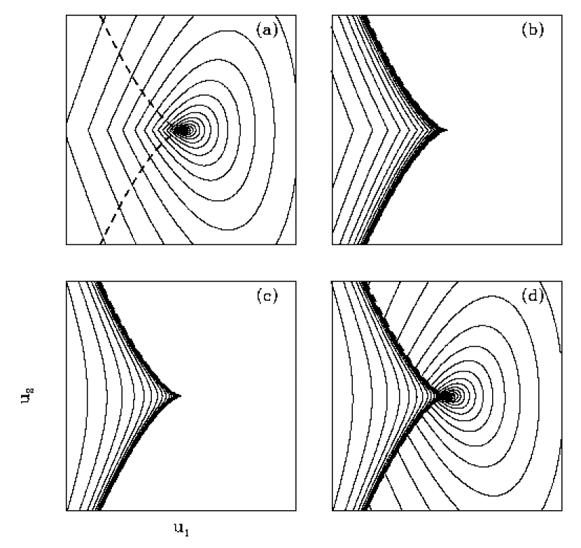
Figure 4: Contour plots of the magnification of the various images as a function of source position, $u$. In each panel, contours are in the interval $\log(\mu)=-1,1$, in logarithmic steps of 0.1, and the dashed line is the caustic. (a) Contours of magnification of the non-divergent, positive-parity image, as a function of $u$. Outside the caustic, this corresponds to $\mu_{\rm loc}^{\rm out}(\mbox{\boldmath$u$})$. Inside the caustic, this corresponds to $\mu^{\rm in}_{1}(\mbox{\boldmath$u$})$ for $u_{2}>0$, and $\mu^{\rm in}_{2}(\mbox{\boldmath$u$})$ for $u_{2}<0$. (b) Contours of the divergent, positive-parity image, which corresponds to $\mu^{\rm in}_{1}(\mbox{\boldmath$u$})$ for $u_{2}<0$, and $\mu^{\rm in}_{2}(\mbox{\boldmath$u$})$ for $u_{2}>0$. (c) Contours of the divergent, negative-parity image, which corresponds to $\mu^{\rm in}_{3}(\mbox{\boldmath$u$})$. (d) Contours of the total magnification. See text for the definitions of $\mu_{\rm loc}^{\rm out}$, $\mu^{\rm in}_{1}$, $\mu^{\rm in}_{2}$, and $\mu^{\rm in}_{3}$

As $u$ approaches the cusp at ${\bf 0}$ from outside the caustic (i.e., the constraint $D(\mbox{\boldmath$u$})>0$ holds for $\mbox{\boldmath$u$}\neq{\bf 0}$), we have $\theta^{\rm out}_{2}(\mbox{\boldmath$u$})\rightarrow 0$. Consequently, the magnification $\mu_{\rm loc}^{\rm out}$ continuously increases without bound as the cusp is approached from outside. This is unlike the case for a source crosses a fold caustic since then a sudden, infinite, discontinuous-jump occurs in the magnification (for point sources). The continuous increase in $\mu_{\rm loc}^{\rm out}$ is due to a lobe of high-magnification outside the cusp (see Fig. 4, and also pp. 334-335, 480-485 of Petters et al. 2001).

We now consider the magnification of sources on the axes, exterior to the cusp. For sources on the $u_{2}$-axis and outside the cusp, we have ${\rm p}=0$ and (thus) $C(\mbox{\boldmath$u$})=u_{2}^{2}$. The resulting image position is therefore

$$\mbox{\boldmath$\theta$}^{\rm out}(0,u_{2})=\left[-\frac{b}{2c}\left(\frac{2c}{2ac-b^{2}}u_{2}\right)^{2/3},\left(\frac{2c}{2ac-b^{2}}u_{2}\right)^{1/3}\right],$$ (32)

and the magnification is given by,

$$\mu_{\rm loc}^{\rm out}(0,u_{2})\equiv\mu(\mbox{\boldmath$\theta$}^{\rm out}(0,u_{2}))=\left(\frac{u_{r2}}{u_{2}}\right)^{2/3},$$ (33)

where we have defined the characteristic rise scale $u_{r2}$ for trajectories along the $u_{2}$-axis,

$$u_{r2}\equiv\left[\frac{27}{2}c^{2}\left(2ac-b^{2}\right)\right]^{-1/2}.$$ (34)

Thus, the magnification diverges as $u_{2}^{-2/3}$ for $u_{2}\rightarrow 0$.

If the source is on the $u_{1}$-axis and outside the cusp (i.e., $u_{1}>0$), then ${\rm q}=0$. Equation (26) yields $\theta^{\rm out}_{2}(u_{1},0)=0$, so the image position is simply,

$$\mbox{\boldmath$\theta$}^{\rm out}(u_{1},0)=\left(\frac{u_{1}}{c},0\right),$$ (35)

and the magnification is given by,

$$\mu_{\rm loc}^{\rm out}(0,u_{2})\equiv\mu(\mbox{\boldmath$\theta$}^{\rm out}(u_{1},0))=\frac{|u_{r1}|}{u_{1}},$$ (36)

where we have defined the rise scale $u_{r1}$,

$$u_{r1}\equiv b^{-1}.$$ (37)

Hence, the magnification diverges as $u_{1}^{-1}$ for $u_{1}\rightarrow 0$.

For a source moving along a path $\mbox{\boldmath$u$}(t)$ (not necessarily rectilinear) lying outside the cusp, the local image centroid follows the motion of the lensed image $\mbox{\boldmath$\theta$}^{\rm out}(\mbox{\boldmath$u$}(t))$ (see the path of ${\mbox{\boldmath$\theta$}}^{\rm out}$ in Figure 1), i.e.,

$${\mbox{\boldmath$\theta$}}_{\rm loc}^{\rm out}(\mbox{\boldmath$u$}(t))=\mbox{\boldmath$\theta$}^{\rm out}(\mbox{\boldmath$u$}(t)).$$ (38)

Observe that ${\mbox{\boldmath$\theta$}}_{\rm loc}^{\rm out}({\bf 0})={\bf 0}$. Figures 1 (b) and (f) illustrate the trajectories of the image and centroid, respectively, for a source in rectilinear motion.

Let us now consider the behavior of the lensed image ${\mbox{\boldmath$\theta$}}^{\rm out}$ when the source at $u$ approaches the caustic. First, as $u$ approaches the cusp ${\bf 0}$ from outside, we obtain ${\mbox{\boldmath$\theta$}}^{\rm out}(\mbox{\boldmath$u$})\rightarrow{\bf 0}$. Second, at a point $\mbox{\boldmath$u$}_{0}=(u_{1}^{0},u_{2}^{0})$ on one of the fold arcs meeting the cusp, equation (26) shows that $\theta^{\rm out}_{2}(\mbox{\boldmath$u$}_{0})=2(-{\rm q}_{0}/2)^{1/3}.$ Since $D(\mbox{\boldmath$u$}_{0})=0$, it follows from equation (25) that

$$\frac{-4{\rm p}_{0}}{3}=4\left(\frac{{\rm q}_{0}}{2}\right)^{\frac{2}{3}}=\left[\theta^{\rm out}_{2}(\mbox{\boldmath$u$}_{0})\right]^{2},$$ (39)

where ${\rm p}_{0}={\rm p}(u_{1}^{0})$ and ${\rm q}_{0}={\rm q}(u_{2}^{0})$. Note that equation (39) implies $-{\rm p}_{0}>0$, which yields

$$bu_{1}^{0}<0$$ (40)

(since $2ac-b^{2}>0$). Hence, the limiting position of $\mbox{\boldmath$\theta$}^{\rm out}(\mbox{\boldmath$u$})$ as $\mbox{\boldmath$u$}\rightarrow\mbox{\boldmath$u$}_{0}$ from outside the caustic is

$${\mbox{\boldmath$\theta$}}^{\rm out}(\mbox{\boldmath$u$}_{0})=\left(\frac{u^{0}_{1}}{c}+\frac{2b}{3c}\ {\rm p}_{0},\ 2\left(\frac{-{\rm q}_{0}}{2}\right)^{\frac{1}{3}}\right).$$ (41)

2.2.3 Local Case: Source on the Caustic

Assume that the source is on the caustic (i.e., $D(\mbox{\boldmath$u$})=0$). If the source is at the cusp point $\mbox{\boldmath$u$}={\bf 0}$, then

$${\rm p}={\rm q}=0,$$ (42)

and equation (17) has a real triple root, $\mbox{\boldmath$\theta$}_{2}({\bf 0})=0$. This yields an infinitely magnified lensed image at the origin of the lens plane. Consequently, for a source on the cusp, the local image centroid is at the origin (as can be seen from Eq.[38]):

$${\bf 0}=\mbox{\boldmath$\theta$}^{\rm out}({\bf 0})={\mbox{\boldmath$\theta$}}_{\rm loc}^{\rm on}({\bf 0}).$$ (43)

If the source is at a point $\mbox{\boldmath$u$}_{0}=(u_{1}^{0},u^{0}_{2})$ on one of the fold arcs abutting the cusp (i.e., $D(\mbox{\boldmath$u$}_{0})=0$ and $\mbox{\boldmath$u$}_{0}\neq{\bf 0}$), then

$${\rm p}_{0}{\rm q}_{0}\neq 0,$$ (44)

so equation (17) has two real roots, one a simple zero and the other a double zero:

$$\theta^{\rm fold,s}_{2}(\mbox{\boldmath$u$}_{0})=2\left(\frac{-{\rm q}_{0}}{2}\right)^{\frac{1}{3}},\qquad\theta^{\rm fold,d}_{2}(\mbox{\boldmath$u$}_{0})=-\left(\frac{-{\rm q}_{0}}{2}\right)^{\frac{1}{3}}.$$ (45)

The corresponding lensed images are as follows (since $D(\mbox{\boldmath$u$}_{0})=0$):

$$\mbox{\boldmath$\theta$}^{\rm fold,d}(\mbox{\boldmath$u$}_{0}) \equiv \left(\frac{u_{1}^{0}}{c}+\frac{b}{6c}\ {\rm p}_{0},-\left(\frac{-{\rm q}_{0}}{2}\right)^{\frac{1}{3}}\right),$$ (46)

$$\mbox{\boldmath$\theta$}^{\rm fold,s}(\mbox{\boldmath$u$}_{0}) \equiv \left(\frac{u_{1}^{0}}{c}+\frac{2b}{3c}\ {\rm p}_{0},2\left(\frac{-{\rm q}_{0}}{2}\right)^{\frac{1}{3}}\right)=\mbox{\boldmath$\theta$}^{\rm out}(\mbox{\boldmath$u$}_{0}).$$ (47)

Note that $\mbox{\boldmath$\theta$}^{\rm fold,d}({\bf 0})={\bf 0}=\mbox{\boldmath$\theta$}^{\rm fold,s}({\bf 0})$ and the rightmost equality in equation (47) is a consequence of equation (41).

Using equation (20), equation (45), and $D(\mbox{\boldmath$u$}_{0})=0$, we get

$$\mathop{\rm det}\nolimits A(\mbox{\boldmath$\theta$}^{\rm fold,s}(\mbox{\boldmath$u$}_{0})) = bu^{0}_{1}-2(2ac-b^{2}){\rm p}_{0}=-3bu^{0}_{1}>0,$$ (48)

$$\mathop{\rm det}\nolimits A(\mbox{\boldmath$\theta$}^{\rm fold,d}(\mbox{\boldmath$u$}_{0})) = bu^{0}_{1}-\frac{1}{2}(2ac-b^{2}){\rm p}_{0}=0,$$ (49)

where the positive condition follows from equation (40). In other words, the image $\mbox{\boldmath$\theta$}^{\rm fold,d}(\mbox{\boldmath$u$}_{0})$ has infinite magnification and so is located on the critical curve. On the other hand, the image $\mbox{\boldmath$\theta$}^{\rm fold,s}(\mbox{\boldmath$u$}_{0})$ is finitely magnified and has positive parity:

$$\mu_{\rm loc}^{\rm fold,s}(\mbox{\boldmath$u$}_{0})\equiv\mu_{\rm loc}(\mbox{\boldmath$\theta$}^{\rm fold,s}(\mbox{\boldmath$u$}_{0}))=\frac{1}{3|bu_{1}^{0}|}=\frac{-1}{3bu_{1}^{0}},$$ (50)

where the rightmost equality follows from equation (40). Now, the root $\theta^{\rm fold,s}_{2}(\mbox{\boldmath$u$}_{0})$ determines the caustic point $\mbox{\boldmath$u$}^{\rm fold,s}_{c}=(u^{\rm fold,s}_{c,1},u^{\rm fold,s}_{c,2}),$ where

$$u^{\rm fold,s}_{c,1}=\frac{3(b^{2}-2ac)}{2b}[\theta^{\rm fold,s}_{2}(\mbox{\boldmath$u$}_{0})]^{2},\qquad u^{\rm fold,s}_{c,2}=\frac{b^{2}-2ac}{c}[\theta^{\rm fold,s}_{2}(\mbox{\boldmath$u$}_{0})]^{3}.$$ (51)

By equation (45), we have

$$u^{\rm fold,s}_{c,1}=4u^{0}_{1}.$$ (52)

Consequently, the horizontal distance from the source at the fold point $\mbox{\boldmath$u$}_{0}$ to the caustic point $\mbox{\boldmath$u$}^{\rm fold,s}_{c}$ is nonzero:

$$\Delta u^{\rm fold,s}_{1,\vdash}\equiv|u^{0}_{1}-u^{\rm fold,s}_{c,1}|=3|u^{0}_{1}|\neq 0.$$ (53)

By equation (24) or (48), the magnification of $\mbox{\boldmath$\theta$}^{\rm fold,s}(\mbox{\boldmath$u$}_{0})$ can be expressed as

$$\mu_{\rm loc}^{\rm fold,s}(\mbox{\boldmath$u$}_{0})=\frac{1}{|b|\Delta u^{\rm fold,s}_{1,\vdash}}.$$ (54)

In other words, the magnification of $\mbox{\boldmath$\theta$}^{\rm fold,s}(\mbox{\boldmath$u$}_{0})$ is not inversely proportional to the horizontal (or ordinary) distance from $\mbox{\boldmath$u$}_{0}$ to the caustic (which is zero since the source sits on the caustic), rather from $\mbox{\boldmath$u$}_{0}$ to the caustic point $\mbox{\boldmath$u$}^{\rm fold,s}_{c}$. Analogous to $\theta^{\rm fold,s}_{2}(\mbox{\boldmath$u$}_{0})$, the root $\theta^{\rm fold,d}_{2}(\mbox{\boldmath$u$}_{0})$ in equation (45) yields a caustic point $\mbox{\boldmath$u$}^{\rm fold,d}_{c}=(u^{\rm fold,d}_{c,1},u^{\rm fold,d}_{c,2})$. Since

$$u^{\rm fold,d}_{c,1}=\frac{3(b^{2}-2ac)}{2b}[\theta^{\rm fold,d}_{2}(\mbox{\boldmath$u$}_{0})]^{2}=u^{0}_{1},$$ (55)

the horizontal distance from $\mbox{\boldmath$u$}_{0}$ to $\mbox{\boldmath$u$}^{\rm fold,d}_{c}$ is zero,

$$\Delta u^{\rm fold,d}_{1,\vdash}=|u^{0}_{1}-u^{\rm fold,d}_{c,1}|=0.$$ (56)

Since $\mu_{\rm loc}^{\rm fold,d}(\mbox{\boldmath$u$}_{0})=1/(|b|\Delta u^{\rm fold,d}_{1,\vdash})$, the vanishing of the horizontal distance gives the earlier result that $\mbox{\boldmath$\theta$}^{\rm fold,d}(\mbox{\boldmath$u$}_{0})$ is infinitely magnified.

As $u$ approaches a fold point $\mbox{\boldmath$u$}_{0}$ from outside the caustic, we have $D(\mbox{\boldmath$u$})\rightarrow 0$ and $\theta^{\rm out}_{2}(\mbox{\boldmath$u$})\rightarrow\theta^{\rm fold,s}_{2}(\mbox{\boldmath$u$}_{0})$ (using Eq.[27]). This implies that the outside local image centroid obeys

$${\mbox{\boldmath$\theta$}}_{\rm loc}^{\rm out}(\mbox{\boldmath$u$})\rightarrow\mbox{\boldmath$\theta$}^{\rm fold,s}(\mbox{\boldmath$u$}_{0}).$$ (57)

However, when $u$ reaches $\mbox{\boldmath$u$}_{0}$, the centroid ${\mbox{\boldmath$\theta$}}_{\rm loc}^{\rm out}(\mbox{\boldmath$u$}_{0})$ not only meets $\mbox{\boldmath$\theta$}^{\rm fold,s}(\mbox{\boldmath$u$}_{0})$, but also the infinitely magnified image $\mbox{\boldmath$\theta$}^{\rm fold,d}(\mbox{\boldmath$u$}_{0})$. The latter image suddenly appears when $\mbox{\boldmath$u$}=\mbox{\boldmath$u$}_{0}$ and dominates $\mbox{\boldmath$\theta$}^{\rm fold,s}(\mbox{\boldmath$u$}_{0})$ in magnification. This causes the image centroid to have a double-value (see Eq.[79] below) and creates a discontinuous jump from $\mbox{\boldmath$\theta$}^{\rm fold,s}(\mbox{\boldmath$u$}_{0})$ to $\mbox{\boldmath$\theta$}^{\rm fold,d}(\mbox{\boldmath$u$}_{0})$. Further discussion of this jump discontinuity will be given below (see equation Section 2.3.2 and Figure 2).

2.2.4 Local Case: Source Inside the Cusp

For sources inside and near the cusp (i.e., $D(\mbox{\boldmath$u$})<0$), equation (17) has three real simple roots:

$$\theta^{\rm in,1}_{2}(\mbox{\boldmath$u$})=2\sqrt{\frac{-{\rm p}}{3}}\cos\left[\frac{\vartheta(\mbox{\boldmath$u$})}{3}\right],\hskip 36.135pt\theta^{\rm in,2}_{2}(\mbox{\boldmath$u$})=-2\sqrt{\frac{-{\rm p}}{3}}\cos\left[\frac{\vartheta(\mbox{\boldmath$u$})-\pi}{3}\right],$$

$$\theta^{\rm in,3}_{2}(\mbox{\boldmath$u$})=-2\sqrt{\frac{-{\rm p}}{3}}\cos\left[\frac{\vartheta(\mbox{\boldmath$u$})+\pi}{3}\right],$$

(58)

where

$$\vartheta(\mbox{\boldmath$u$})=\cos^{-1}\left[\frac{(-{\rm q}/2)}{\sqrt{(-{\rm p}/3)^{3}}}\right].$$ (59)

Since $D(\mbox{\boldmath$u$})<0$, it follows that $({\rm p}/3)^{3}<-({\rm q}/2)^{2}\leq 0$, which yields ${\rm p}<0$ and $bu_{1}<0$ (since $2ac-b^{2}>0$). In addition, we have $|{\rm q}/2|/\sqrt{(-{\rm p}/3)^{3}}<1$, or, $-1<(-{\rm q}/2)/\sqrt{(-{\rm p}/3)^{3}}<1$. Consequently,

$$0<\vartheta(\mbox{\boldmath$u$})<\pi$$ (60)

for $u$ inside the caustic. The values $\vartheta(\mbox{\boldmath$u$})=0$ and $\vartheta(\mbox{\boldmath$u$})=\pi$ occur when $u$ is on the top and bottom fold arcs, respectively, that abut the cusp (see discussion below). The value $\vartheta(\mbox{\boldmath$u$})=\pi/2$ is for $u$ on the $u_{1}$-axis inside the caustic.

A source inside and near the cusp has three local images determined by equation (58):

$$\mbox{\boldmath$\theta$}^{\rm in,1}(\mbox{\boldmath$u$}) = \left(\frac{u_{1}}{c}+\frac{2b}{3c}{\rm p}\cos^{2}\left[\frac{\vartheta(\mbox{\boldmath$u$})}{3}\right],2\sqrt{\frac{-{\rm p}}{3}}\cos\left[\frac{\vartheta(\mbox{\boldmath$u$})}{3}\right]\right),$$

$$\mbox{\boldmath$\theta$}^{\rm in,2}(\mbox{\boldmath$u$}) = \left(\frac{u_{1}}{c}+\frac{2b}{3c}{\rm p}\cos^{2}\left[\frac{\vartheta(\mbox{\boldmath$u$})-\pi}{3}\right],-2\sqrt{\frac{-{\rm p}}{3}}\cos\left[\frac{\vartheta(\mbox{\boldmath$u$})-\pi}{3}\right]\right),$$

$$\mbox{\boldmath$\theta$}^{\rm in,3}(\mbox{\boldmath$u$}) = \left(\frac{u_{1}}{c}+\frac{2b}{3c}{\rm p}\cos^{2}\left[\frac{\vartheta(\mbox{\boldmath$u$})+\pi}{3}\right],-2\sqrt{\frac{-{\rm p}}{3}}\cos\left[\frac{\vartheta(\mbox{\boldmath$u$})+\pi}{3}\right]\right).$$

We saw that the condition $D(\mbox{\boldmath$u$})<0$ yields $bu_{1}<0$ and $0<\vartheta(\mbox{\boldmath$u$})<\pi$ for sources inside the caustic. The latter, implies

$$\mathop{\rm det}\nolimits A(\mbox{\boldmath$\theta$}^{\rm in,1}(\mbox{\boldmath$u$})) = bu_{1}\left[1-4\cos^{2}\left(\frac{\vartheta(\mbox{\boldmath$u$})}{3}\right)\right]>0,$$

$$\mathop{\rm det}\nolimits A(\mbox{\boldmath$\theta$}^{\rm in,2}(\mbox{\boldmath$u$})) = bu_{1}\left[1-4\cos^{2}\left(\frac{\vartheta(\mbox{\boldmath$u$})-\pi}{3}\right)\right]>0,$$

$$\mathop{\rm det}\nolimits A(\mbox{\boldmath$\theta$}^{\rm in,3}(\mbox{\boldmath$u$})) = bu_{1}\left[1-4\cos^{2}\left(\frac{\vartheta(\mbox{\boldmath$u$})+\pi}{3}\right)\right]<0.$$

In other words, the lensed images $\mbox{\boldmath$\theta$}^{\rm in,1}$ and $\mbox{\boldmath$\theta$}^{\rm in,2}$ have positive parity, while $\mbox{\boldmath$\theta$}^{\rm in,3}$ has negative parity. It is useful to note that

$$\mathop{\rm det}\nolimits A(\mbox{\boldmath$\theta$}^{\rm in,1}(\mbox{\boldmath$u$})) = 0,~{}{\rm for}~{}\theta=\pi,$$

$$\mathop{\rm det}\nolimits A(\mbox{\boldmath$\theta$}^{\rm in,2}(\mbox{\boldmath$u$})) = 0,~{}{\rm for}~{}\theta=0,$$

$$\mathop{\rm det}\nolimits A(\mbox{\boldmath$\theta$}^{\rm in,3}(\mbox{\boldmath$u$})) = 0,~{}{\rm for}~{}\theta=0,\pi.$$

Let us now consider the behavior of three images in equation (2.2.4) near the caustic — see Figures 2 and 3. Equation (2.2.4) shows that as $\mbox{\boldmath$u$}\rightarrow{\bf 0}$ (source approaches the cusp) from inside the caustic, we obtain

$$\mbox{\boldmath$\theta$}^{\rm in,\ell}(\mbox{\boldmath$u$})\rightarrow{\bf 0},\qquad\ell=1,2,3,$$ (64)

i.e., all three images merge at the point on the critical curve that maps to the cusp. We now investigate the image behavior as the source approaches a fold caustic. There are two fold arcs abutting the cusp, one in lying above the $u_{1}$-axis and the other below. If the source is on one of these fold arcs, then $D(\mbox{\boldmath$u$})=0$ and ${\rm p}{\rm q}\neq 0$. At a point $\mbox{\boldmath$u$}_{0}$ on the fold arc above the $u_{1}$-axis, we have $(-{\rm q}_{0}/2)=\sqrt{(-{\rm p}_{0}/3)^{3}}$, which yields $\vartheta(\mbox{\boldmath$u$}_{0})=0$. By equation (LABEL:x123), as the source position $u$ approaches $\mbox{\boldmath$u$}_{0}$ from the interior of the cusped caustic, we have

$$\mbox{\boldmath$\theta$}^{\rm in,1}(\mbox{\boldmath$u$})\longrightarrow\mbox{\boldmath$\theta$}^{\rm fold,s}(\mbox{\boldmath$u$}_{0}),\hskip 21.68121pt\mbox{\boldmath$\theta$}^{\rm in,2}(\mbox{\boldmath$u$})\longrightarrow\mbox{\boldmath$\theta$}^{\rm fold,d}(\mbox{\boldmath$u$}_{0}),\hskip 21.68121pt\mbox{\boldmath$\theta$}^{\rm in,3}(\mbox{\boldmath$u$})\longrightarrow\mbox{\boldmath$\theta$}^{\rm fold,d}(\mbox{\boldmath$u$}_{0}).$$ (65)

If the source crosses the fold transversely through the point $\mbox{\boldmath$u$}_{0}$ and continues on to outside the fold, then the lensed image moving along $\mbox{\boldmath$\theta$}^{\rm in,1}(\mbox{\boldmath$u$})$ passes through $\mbox{\boldmath$\theta$}^{\rm fold,s}(\mbox{\boldmath$u$}_{0})$ and continues along $\mbox{\boldmath$\theta$}^{\rm out}(\mbox{\boldmath$u$})$. In addition, the other two images moving along $\mbox{\boldmath$\theta$}^{\rm in,2}(\mbox{\boldmath$u$})$ and $\mbox{\boldmath$\theta$}^{\rm in,3}(\mbox{\boldmath$u$})$ merge into a single lensed image at $\mbox{\boldmath$\theta$}^{\rm fold,d}(\mbox{\boldmath$u$}_{0})$, and then disappear as the source moves outside the caustic. These results are depicted in Figure 2(b). Similar results occur if the source travels from outside the caustic approaching a point $\mbox{\boldmath$u$}_{0}$ lying on the fold arc below the $u_{1}$-axis, see Figure 3(b). In this case, $(-{\rm q}_{0}/2)=-\sqrt{(-{\rm p}_{0}/3)^{3}}$, which yields $\vartheta(\mbox{\boldmath$u$}_{0})=\pi$. As the source approaches $\mbox{\boldmath$u$}_{0}$ from outside, there is one image locally and the image moves along $\mbox{\boldmath$\theta$}^{\rm out}$. Equation (LABEL:x123) shows that as $\mbox{\boldmath$u$}\rightarrow\mbox{\boldmath$u$}_{0}$ from outside the caustic, we have

$$\mbox{\boldmath$\theta$}^{\rm out}(\mbox{\boldmath$u$})\longrightarrow\mbox{\boldmath$\theta$}^{\rm fold,s}(\mbox{\boldmath$u$}_{0})=\mbox{\boldmath$\theta$}^{\rm in,2}(\mbox{\boldmath$u$}_{0}).$$ (66)

When the source reaches $\mbox{\boldmath$u$}_{0}$, an infinitely magnified lensed image $\mbox{\boldmath$\theta$}^{\rm fold,d}(\mbox{\boldmath$u$}_{0})$ suddenly appears. As the source moves transversely through $\mbox{\boldmath$u$}_{0}$ and enters inside the caustic, equation (LABEL:x123) yields that $\mbox{\boldmath$\theta$}^{\rm fold,d}(\mbox{\boldmath$u$}_{0})$ splits into two images that move along $\mbox{\boldmath$\theta$}^{\rm in,1}(\mbox{\boldmath$u$})$ and $\mbox{\boldmath$\theta$}^{\rm in,3}(\mbox{\boldmath$u$})$. Equivalently, if a source at $u$ moves from inside the caustic to a point $\mbox{\boldmath$u$}_{0}$ on the fold arc below the $u_{1}$-axis, we have that $\mbox{\boldmath$\theta$}^{\rm in,1}(\mbox{\boldmath$u$})$ and $\mbox{\boldmath$\theta$}^{\rm in,3}(\mbox{\boldmath$u$})$ merge at $\mbox{\boldmath$\theta$}^{\rm fold,d}(\mbox{\boldmath$u$}_{0})$:

$$\mbox{\boldmath$\theta$}^{\rm in,2}(\mbox{\boldmath$u$})\longrightarrow\mbox{\boldmath$\theta$}^{\rm fold,s}(\mbox{\boldmath$u$}_{0}),\hskip 7.22743pt\mbox{\boldmath$\theta$}^{\rm in,1}(\mbox{\boldmath$u$})\longrightarrow\mbox{\boldmath$\theta$}^{\rm fold,d}(\mbox{\boldmath$u$}_{0}),\hskip 7.22743pt\mbox{\boldmath$\theta$}^{\rm in,3}(\mbox{\boldmath$u$})\longrightarrow\mbox{\boldmath$\theta$}^{\rm fold,d}(\mbox{\boldmath$u$}_{0}).$$ (67)

The magnifications of the images $\mbox{\boldmath$\theta$}^{\rm in,\ell}(\mbox{\boldmath$u$})$ are

$$\mu^{\rm in}_{\ell}(\mbox{\boldmath$u$})\equiv\mu(\mbox{\boldmath$\theta$}^{\rm in,\ell}(\mbox{\boldmath$u$}))=\frac{1}{|b|\Delta u^{\rm in,\ell}_{1,\vdash}},\qquad\ell=1,2,3,$$ (68)

where the horizontal distances are given by

$$\Delta u^{\rm in,1}_{1,\vdash}=|u_{1}\left(1-4\cos^{2}[\vartheta(\mbox{\boldmath$u$})/3]\right)|,\qquad\Delta u^{\rm in,2}_{1,\vdash}=|u_{1}\left(1-4\cos^{2}[(\vartheta(\mbox{\boldmath$u$})-\pi)/3]\right)|,$$

$$\Delta u^{\rm in,3}_{1,\vdash}=|u_{1}\left(1-4\cos^{2}[(\vartheta(\mbox{\boldmath$u$})+\pi)/3]\right)|.$$

Observe that if the source is inside the caustic, but on the $u_{1}$-axis, then $\vartheta(u_{1},0)=\pi/2$, which yields

$$\mu^{\rm in}_{1}(u_{1},0)=\frac{1}{2|bu_{1}|}=\frac{-1}{2bu_{1}},\qquad\mu^{\rm in}_{2}(u_{1},0)=\frac{1}{2|bu_{1}|}=\frac{-1}{2bu_{1}},\qquad\mu^{\rm in}_{3}(u_{1},0)=\frac{1}{|bu_{1}|}=\frac{-1}{bu_{1}}.$$ (70)

In other words, the magnification is inversely proportional to the distance of the source (on the $u_{1}$-axis) from the cusp. The magnification of the images are shown in Figures 2(b) and 3(b) for a source in rectilinear motion. It follows from equation (70) that

$$\mu^{\rm in}_{3}(u_{1},0)=\mu^{\rm in}_{1}(u_{1},0)+\mu^{\rm in}_{2}(u_{1},0).$$ (71)

In fact, this relationship holds for any position $u$ inside and near the cusp (e.g., Schneider & Weiss 1992; Zakharov 1995, 1999):

$$\mu^{\rm in}_{3}(\mbox{\boldmath$u$})=\mu^{\rm in}_{1}(\mbox{\boldmath$u$})+\mu^{\rm in}_{2}(\mbox{\boldmath$u$}),$$ (72)

where $D(\mbox{\boldmath$u$})<0$. Hence, the total magnification of the three local images is

$$\mu_{\rm loc}^{\rm in}(\mbox{\boldmath$u$})=\mu^{\rm in}_{1}(\mbox{\boldmath$u$})+\mu^{\rm in}_{2}(\mbox{\boldmath$u$})+\mu^{\rm in}_{3}(\mbox{\boldmath$u$})=2\left[\mu^{\rm in}_{1}(\mbox{\boldmath$u$})+\mu^{\rm in}_{2}(\mbox{\boldmath$u$})\right].$$ (73)

The image centroid of the three images for source positions inside and near the cusp is given by

$${\mbox{\boldmath$\theta$}}_{\rm loc}^{\rm in}=\frac{\mu^{\rm in}_{1}\mbox{\boldmath$\theta$}^{\rm in,1}+\mu^{\rm in}_{2}\mbox{\boldmath$\theta$}^{\rm in,2}+\mu^{\rm in}_{3}\mbox{\boldmath$\theta$}^{\rm in,3}}{\mu^{\rm in}_{1}+\mu^{\rm in}_{2}+\mu^{\rm in}_{3}}=\frac{1}{2}\left[{\mbox{\boldmath$\theta$}}_{\rm loc}^{\rm in(1,2)}+\mbox{\boldmath$\theta$}^{\rm in,3}\right],$$ (74)

where ${\mbox{\boldmath$\theta$}}_{\rm loc}^{\rm in(1,2)}$ is the centroid of the images $\mbox{\boldmath$\theta$}^{\rm in,1}$ and $\mbox{\boldmath$\theta$}^{\rm in,2}$, i.e.,

$${\mbox{\boldmath$\theta$}}_{\rm loc}^{\rm in(1,2)}=\frac{\mu^{\rm in,1}\mbox{\boldmath$\theta$}^{\rm in,1}+\mu^{\rm in,2}\mbox{\boldmath$\theta$}^{\rm in,2}}{\mu^{\rm in,1}+\mu^{\rm in,2}}.$$ (75)

The image centroid for a source in rectilinear motion is shown in Figures 2(f) and 3(f).

Equation (65) shows that as $\mbox{\boldmath$u$}\rightarrow\mbox{\boldmath$u$}_{0}$ from inside the caustic, where $\mbox{\boldmath$u$}_{0}$ lies on the fold arc above the $u_{1}$-axis, we obtain $\mu^{\rm in,1}(\mbox{\boldmath$u$})\rightarrow\mu^{\rm fold,s}_{\rm loc}(\mbox{\boldmath$u$}_{0}),$ where $0<\mu^{\rm fold,s}_{\rm loc}(\mbox{\boldmath$u$}_{0})<\infty$, and $\mu^{\rm in,2}(\mbox{\boldmath$u$})\rightarrow\infty$. This yields

$$\frac{\mu^{\rm in,1}(\mbox{\boldmath$u$})}{\mu^{\rm in,1}(\mbox{\boldmath$u$})+\mu^{\rm in,2}(\mbox{\boldmath$u$})}\rightarrow 0,\qquad\frac{\mu^{\rm in,2}(\mbox{\boldmath$u$})}{\mu^{\rm in,1}(\mbox{\boldmath$u$})+\mu^{\rm in,2}(\mbox{\boldmath$u$})}\rightarrow 1\qquad\quad\mbox{as}\ \mbox{\boldmath$u$}\rightarrow\mbox{\boldmath$u$}_{0}.$$ (76)

Similarly, equation (67) shows that if $\mbox{\boldmath$u$}_{0}$ is on the fold arc below the $u_{1}$-axis, then $\mu^{\rm in,2}(\mbox{\boldmath$u$})\rightarrow\mu^{\rm fold,s}_{\rm loc}(\mbox{\boldmath$u$}_{0})$ and $\mu^{\rm in,1}(\mbox{\boldmath$u$})\rightarrow\infty$. Consequently,

$$\frac{\mu^{\rm in,1}(\mbox{\boldmath$u$})}{\mu^{\rm in,1}(\mbox{\boldmath$u$})+\mu^{\rm in,2}(\mbox{\boldmath$u$})}\rightarrow 1,\qquad\frac{\mu^{\rm in,2}(\mbox{\boldmath$u$})}{\mu^{\rm in,1}(\mbox{\boldmath$u$})+\mu^{\rm in,2}(\mbox{\boldmath$u$})}\rightarrow 0\qquad\quad\mbox{as}\ \mbox{\boldmath$u$}\rightarrow\mbox{\boldmath$u$}_{0}.$$ (77)

It follows that as $\mbox{\boldmath$u$}\rightarrow\mbox{\boldmath$u$}_{0}$ from inside the caustic, we have ${\mbox{\boldmath$\theta$}}_{\rm loc}^{\rm in(1,2)}(\mbox{\boldmath$u$})\rightarrow\mbox{\boldmath$\theta$}^{\rm fold,d}$ and $\mbox{\boldmath$\theta$}^{\rm in,3}(\mbox{\boldmath$u$})\rightarrow\mbox{\boldmath$\theta$}^{\rm fold,d}$. Hence,

$${\mbox{\boldmath$\theta$}}_{\rm loc}^{\rm in}(\mbox{\boldmath$u$})\rightarrow\mbox{\boldmath$\theta$}^{\rm fold,d}(\mbox{\boldmath$u$}_{0}).$$ (78)

as $\mbox{\boldmath$u$}\rightarrow\mbox{\boldmath$u$}_{0}$ from inside the caustic. Equations (57) and (78) then show that for $\mbox{\boldmath$u$}=\mbox{\boldmath$u$}_{0}$, the local image centroid is double valued and so has a jump discontinuity (Figures 2(f) and 3(f)):

$${\mbox{\boldmath$\theta$}}_{\rm loc}(\mbox{\boldmath$u$}_{0})=\{\mbox{\boldmath$\theta$}^{\rm fold,s}(\mbox{\boldmath$u$}_{0}),\ \mbox{\boldmath$\theta$}^{\rm fold,d}(\mbox{\boldmath$u$}_{0})\}.$$ (79)

2.2.5 Local Case: Summary of Local Results

The magnification of the local images associated with a source at angular vector position $u$ near the cusp can now be summarized as follows:

$$\mu_{\rm loc}(\mbox{\boldmath$u$})=\left\{\begin{array}[]{ll}\mu_{\rm loc}^{\rm out}(\mbox{\boldmath$u$})&\quad\mbox{$\mbox{\boldmath$u$}$ outside caustic},\\ \\ \infty,&\quad\mbox{$\mbox{\boldmath$u$}$ on caustic},\\ \\ 2\left[\mu^{\rm in}_{1}(\mbox{\boldmath$u$})+\mu^{\rm in}_{2}(\mbox{\boldmath$u$})\right]&\quad\mbox{$\mbox{\boldmath$u$}$ inside caustic},\end{array}\right.$$ (80)

where the magnifications $\mu_{\rm loc}^{\rm out}$ and $\mu^{\rm in}_{\ell}$, $\ell=1,2$, are given by equations (30) and (68), respectively. These magnifications are shown as a function of source position in Figures 1-4. The image centroid is given by:

$${\mbox{\boldmath$\theta$}}_{\rm loc}(\mbox{\boldmath$u$})=\left\{\begin{array}[]{ll}\mbox{\boldmath$\theta$}^{\rm out}(\mbox{\boldmath$u$})&\quad\mbox{$\mbox{\boldmath$u$}$ outside caustic},\\ \\ \left\{{\mbox{\boldmath$\theta$}}_{\rm loc}^{\rm fold,d}(\mbox{\boldmath$u$}_{0}),\ {\mbox{\boldmath$\theta$}}_{\rm loc}^{\rm fold,s}(\mbox{\boldmath$u$}_{0})\right\},&\quad\mbox{$\mbox{\boldmath$u$}=\mbox{\boldmath$u$}_{0}$ on fold arc},\\ \\ {\bf 0},&\quad\mbox{$\mbox{\boldmath$u$}={\bf 0}$ on cusp},\\ \\ (1/2)\left[{\mbox{\boldmath$\theta$}}_{\rm loc}^{\rm in(1,2)}(\mbox{\boldmath$u$})+\mbox{\boldmath$\theta$}^{\rm in,3}(\mbox{\boldmath$u$})\right]&\quad\mbox{$\mbox{\boldmath$u$}$ inside caustic},\end{array}\right.$$ (81)

where the angular vector $\mbox{\boldmath$\theta$}^{\rm out}$ is given by equation (28), ${\mbox{\boldmath$\theta$}}_{\rm loc}^{\rm fold,d}$ by equation (46), ${\mbox{\boldmath$\theta$}}_{\rm loc}^{\rm fold,s}$ by equation (47), $\mbox{\boldmath$\theta$}^{\rm in,3}$ by equation (2.2.4), and ${\mbox{\boldmath$\theta$}}_{\rm loc}^{\rm in(1,2)}$ by equation (75). Note that the above equations can be applied to a general (not necessarily rectilinear) source trajectory $\mbox{\boldmath$u$}=\mbox{\boldmath$u$}(t)$. The local centroid is illustrated in Figures 1(f), 2(f), and 3(f) for rectilinear source motion.

2.3 Global Case: Point Sources Near a Cusp

2.3.1 Magnification and Centroid of All Images

Suppose that the source moves rectilinearly, i.e., its trajectory is given by

$$\mbox{\boldmath$u$}(t)=\mbox{\boldmath$u$}_{c}+(t-t_{c})\dot{\mbox{\boldmath$u$}},$$ (82)

where $\mbox{\boldmath$u$}_{c}$ is the position at which the source intersects at time $t=t_{c}$ the tangent line to the cusp, which coincides with the the $u_{1}$-axis, and $\dot{\mbox{\boldmath$u$}}$ is the constant angular velocity vector of the source,

$$\dot{\mbox{\boldmath$u$}}=\left(\frac{\cos\phi}{t_{\rm E}},\frac{\sin\phi}{t_{\rm E}}\right).$$ (83)

Recall that $t_{\rm E}=D_{ol}\theta_{\rm E}/{\mbox{\rm v}}_{\perp}$, where $\theta_{\rm E}$ is the angular Einstein radius and ${\mbox{\rm v}}_{\perp}$ is the proper transverse speed of the lens relative to the observer-source line-of-sight. Here $\phi$ is the angle of the source’s trajectory with respect to the $u_{1}$-axis (i.e., tangent line to the cusp).

As the source moves along the rectilinear path in equation (82), the angular positions of the images unaffiliated with the cusp follow continuous trajectories and their magnifications are positive, finite, and continuous. Moreover, we assume that for source trajectories near the cusp, the image magnifications and positions of the unaffiliated images are slowly varying functions of the source position $u$. Denote the centroid and total magnification of the unaffiliated images by $\mbox{\boldmath$\theta$}_{0}$ and $\mu_{0}$, respectively. Then the magnification $\mu_{\rm tot}$ and image centroid ${\mbox{\boldmath$\theta$}}_{\rm cl}$ of all the images are given by

$$\mu_{\rm tot}(\mbox{\boldmath$u$})=\mu_{\rm loc}(\mbox{\boldmath$u$})+\mu_{0}(\mbox{\boldmath$u$})$$ (84)

and

$${\mbox{\boldmath$\theta$}}_{\rm cl}(\mbox{\boldmath$u$})=\frac{1}{\mu_{tot}(\mbox{\boldmath$u$})}\left[\mu_{\rm loc}(\mbox{\boldmath$u$}){\mbox{\boldmath$\theta$}}_{\rm loc}(\mbox{\boldmath$u$})+\mu_{0}(\mbox{\boldmath$u$})\mbox{\boldmath$\theta$}_{0}(\mbox{\boldmath$u$})\right].$$ (85)

The photometric and astrometric observables $\mu_{\rm tot}$ and ${\mbox{\boldmath$\theta$}}_{\rm loc}$, respectively, can be expressed as functions of time by replacing $u$ in equations (84) and (85) by the rectilinear source trajectory $\mbox{\boldmath$u$}(t)$ in equation (82), and Taylor expanding $\mbox{\boldmath$\theta$}_{0}$ and $\mu_{0}$ to first order about the crossing time $t=t_{c}$ of the tangent line to the cusp. This yields:

$$\mu_{\rm tot}(t)=\mu_{\rm loc}(t)+\mu_{0}(t),$$ (86)

where $\mu_{\rm loc}(t)=\mu_{\rm loc}(\mbox{\boldmath$u$}(t))$ and $\mu_{0}(t)=\mu_{0,c}+(t-t_{c})\dot{\mu}_{(0,c)}$ with $\dot{\mu}_{(0,c)}={\rm d}\mu_{0}/{\rm d}t|_{t=t_{c}},$ and

$${\mbox{\boldmath$\theta$}}_{\rm cl}(t)=\frac{1}{\mu_{tot}(t)}\left[\mu_{\rm loc}(t){\mbox{\boldmath$\theta$}}_{\rm loc}(t)+\mu_{0}(t)\mbox{\boldmath$\theta$}_{0}(t)\right],$$ (87)

where ${\mbox{\boldmath$\theta$}}_{\rm loc}(t)={\mbox{\boldmath$\theta$}}_{\rm loc}(\mbox{\boldmath$u$}(t))$ and $\mbox{\boldmath$\theta$}_{0}=\mbox{\boldmath$\theta$}_{0,c}+(t-t_{c})\dot{\mbox{\boldmath$\theta$}}_{(0,c)}$ with $\dot{\mbox{\boldmath$\theta$}}_{(0,c)}={\rm d}\mbox{\boldmath$\theta$}_{0}/{\rm d}t|_{t=t_{c}}.$

2.3.2 Image Centroid Jump-Discontinuity at Fold Crossing

Assume that a source in rectilinear motion $\mbox{\boldmath$u$}(t)$ transversely crosses the point $\mbox{\boldmath$u$}_{0}$ on one of the fold arcs abutting the cusp. As $\mbox{\boldmath$u$}(t)\rightarrow\mbox{\boldmath$u$}_{0}$ from inside (respectively, outside) the cusp, denote the limiting value of the image centroid ${\mbox{\boldmath$\theta$}}_{\rm cl}(\mbox{\boldmath$u$}(t))$ by ${\mbox{\boldmath$\theta$}}_{\rm cl}^{+}(\mbox{\boldmath$u$}_{0})$ (respectively, ${\mbox{\boldmath$\theta$}}_{\rm cl}^{-}(\mbox{\boldmath$u$}_{0})$). The jump-discontinuity vector at $\mbox{\boldmath$u$}_{0}$ for the image centroid and shifted image centroid are the same:

$${\mbox{\boldmath$\theta$}}_{\rm cl}^{\rm jump}(\mbox{\boldmath$u$}_{0})={\mbox{\boldmath$\theta$}}_{\rm cl}^{+}(\mbox{\boldmath$u$}_{0})-{\mbox{\boldmath$\theta$}}_{\rm cl}^{-}(\mbox{\boldmath$u$}_{0})=\delta\mbox{\boldmath$\theta$}_{\rm cl}^{\rm jump}(\mbox{\boldmath$u$}_{0}).$$ (88)

As $\mbox{\boldmath$u$}\rightarrow\mbox{\boldmath$u$}_{0}$ from inside the cusp, we have

$$\frac{\mu_{0}(\mbox{\boldmath$u$})}{\mu_{\rm tot}(\mbox{\boldmath$u$})}\rightarrow\frac{1}{1+\mu_{\rm loc}(\mbox{\boldmath$u$}_{0})/\mu_{0}(\mbox{\boldmath$u$}_{0})}=0,$$ (89)

(since $\mu_{\rm loc}(\mbox{\boldmath$u$})\rightarrow\infty$ and $\mu_{0}(\mbox{\boldmath$u$})$ is generally non-divergent). Therefore, from equation (85), it follows that ${\mbox{\boldmath$\theta$}}_{\rm cl}^{+}(\mbox{\boldmath$u$}_{0})=\mbox{\boldmath$\theta$}^{\rm fold,d}(\mbox{\boldmath$u$}_{0})$, i.e. the contribution from the images not associated with the cusp is negligible. In contrast, as $\mbox{\boldmath$u$}\rightarrow\mbox{\boldmath$u$}_{0}$ from outside the cusp, we have

$$\frac{\mu_{0}(\mbox{\boldmath$u$})}{\mu_{\rm tot}(\mbox{\boldmath$u$})}\rightarrow\frac{1}{1+\mu_{\rm loc}^{\rm out}(\mbox{\boldmath$u$}_{0})/\mu_{0}(\mbox{\boldmath$u$}_{0})}\neq 0,$$ (90)

where the last inequality holds provided that $\mbox{\boldmath$u$}_{0}\neq{\bf 0}$. Thus, we generally have that ${\mbox{\boldmath$\theta$}}_{\rm cl}^{-}(\mbox{\boldmath$u$}_{0})\neq\mbox{\boldmath$\theta$}^{\rm fold,s}(\mbox{\boldmath$u$}_{0})$, and the contribution from images not associated with the cusp can be substantial. However, due to the fact that the magnification of the image exterior to the cusp is $\gg 1$ for positions close to the cusp, it likely a fair approximation to ignore the contribution from the other images. We will therefore assume that $\mu_{\rm loc}^{\rm out}(\mbox{\boldmath$u$}_{0})/\mu_{0}(\mbox{\boldmath$u$}_{0})\gg 1$, and thus ${\mbox{\boldmath$\theta$}}_{\rm cl}^{-}(\mbox{\boldmath$u$}_{0})\simeq\mbox{\boldmath$\theta$}^{\rm fold,s}(\mbox{\boldmath$u$}_{0})$. Consequently,

$${\mbox{\boldmath$\theta$}}_{\rm cl}^{\rm jump}(\mbox{\boldmath$u$}_{0})=\mbox{\boldmath$\theta$}^{\rm fold,d}(\mbox{\boldmath$u$}_{0})-\mbox{\boldmath$\theta$}^{\rm fold,s}(\mbox{\boldmath$u$}_{0})$$ (91)

Since $\mbox{\boldmath$\theta$}^{\rm fold,d}(\mbox{\boldmath$u$}_{0})\neq\mbox{\boldmath$\theta$}^{\rm fold,s}(\mbox{\boldmath$u$}_{0})$, we obtain a discontinuous jump in the image centroid as the source passes through the fold point $\mbox{\boldmath$u$}_{0}$. There is no discontinuous jump if the source passes through the cusp (since ${\mbox{\boldmath$\theta$}}_{\rm cl}^{\rm jump}({\bf 0})={\bf 0}$). Since by equation (25) we have $(-{\rm q}_{0}/2)^{1/3}=\mp(-{\rm p}_{0}/3)^{1/2}$, where the minus (respectively, plus) corresponds to $\mbox{\boldmath$u$}_{0}$ on the fold arc below (respectively, above) the $u_{1}$-axis, equations (46) and (47) yield

$${\mbox{\boldmath$\theta$}}_{\rm cl}^{\rm jump}(\mbox{\boldmath$u$}_{0})=\left(-\frac{b}{2c}{\rm p}_{0},\mp 3\sqrt{\frac{-{\rm p}_{0}}{3}}\right)=\left(\frac{b^{2}u^{0}_{1}}{c(2ac-b^{2})},\mp\sqrt{\frac{-6bu^{0}_{1}}{2ac-b^{2}}}\right),$$ (92)

where as before the $\mp$ signs are for $\mbox{\boldmath$u$}_{0}$ on the respective fold arcs below and above the tangent line to the cusp (i.e., the $u_{1}$-axis). Note that $bu^{0}_{1}<0$ by equation (40).

For $\mbox{\boldmath$u$}_{0}$ sufficiently close to the cusp at ${\bf 0}$, the variable $u^{0}_{1}$ dominates $(u^{0}_{1})^{2}$. We can then approximate the magnitude of the jump as follows:

$$\left|{\mbox{\boldmath$\theta$}}_{\rm cl}^{\rm jump}(\mbox{\boldmath$u$}_{0})\right|=\left[\left(\frac{b^{2}u^{0}_{1}}{c(2ac-b^{2})}\right)^{2}+\frac{-6bu^{0}_{1}}{2ac-b^{2}}\right]^{1/2}\simeq\sqrt{\frac{-6bu^{0}_{1}}{2ac-b^{2}}}.$$ (93)

Therefore, the magnitude of the centroid jump increases as $|u^{0}_{1}|^{1/2}$ for $|u^{0}_{1}|\ll 1$, where $|u^{0}_{1}|$ is the horizontal distance of the caustic point $\mbox{\boldmath$u$}_{0}$ from the cusp. Note that no jump discontinuity occurs for a source passing through the cusp.

2.4 Extended Sources Near a Cusp

2.4.1 Magnification and Image Centroid of Extended Sources

Consider an extended source with surface brightness $S(\mbox{\boldmath$u$})$. The average surface brightness is $\bar{S}\equiv(\pi\rho^{2}_{*})^{-1}\ \int_{\cal{D}}{\rm d}\mbox{\boldmath$u$}\ S(\mbox{\boldmath$u$})$, where ${\cal{D}}$ is the disc-shaped region of the source and $\rho_{*}\equiv\theta_{*}/\theta_{\rm E}$ is the angular source radius $\theta_{*}$ in units of $\theta_{\rm E}$. The magnification of the finite source is then

$$\mu^{\rm fs}={{\int_{\cal{D}}{\rm d}\mbox{\boldmath$u$}S(\mbox{\boldmath$u$})\mu(\mbox{\boldmath$u$})}\over{\int_{\cal{D}}{\rm d}\mbox{\boldmath$u$}S(\mbox{\boldmath$u$})}},$$ (94)

Introduce new coordinates by

$$\mbox{\boldmath$u$}^{\prime}=\frac{\mbox{\boldmath$u$}-{\mbox{\boldmath$u$}}_{\rm cn}}{\rho_{*}},$$ (95)

where ${\mbox{\boldmath$u$}}_{\rm cn}$ is the center of the source. Note that $|u^{\prime}|\leq 1$. Then equation (94) simplifies to

$$\mu^{\rm fs}=\frac{1}{\pi}\int_{D}{\rm d}\mbox{\boldmath$u$}^{\prime}{S_{N}}(\mbox{\boldmath$u$}^{\prime})\mu(\mbox{\boldmath$u$}^{\prime}),$$ (96)

where ${S_{N}}(\mbox{\boldmath$u$})=S(\mbox{\boldmath$u$})/\bar{S}.$ In the case of small source sizes $\theta_{*}\ll\theta_{\rm E}$, the magnification $\mu_{0}(\mbox{\boldmath$u$})$ of the images not associated with the cusp is a slowly varying function of $u$ over the source, which yields

$$\mu_{0}^{\rm fs}\simeq\mu_{0}(\mbox{\boldmath$u$}_{cn})\equiv\mu_{0,{cn}}.$$ (97)

The total finite source magnification becomes

$${\mu_{\rm tot}^{\rm fs}}=\frac{1}{\pi}\int_{\cal{D}}{\rm d}\mbox{\boldmath$u$}^{\prime}{S_{N}}(\mbox{\boldmath$u$}^{\prime})\mu_{\rm tot}(\mbox{\boldmath$u$}^{\prime})=\mu_{\rm loc}^{\rm fs}+\mu_{0,cn},$$ (98)

where

$$\mu_{\rm loc}^{\rm fs}=\frac{1}{\pi}\int_{\cal{D}}{\rm d}\mbox{\boldmath$u$}^{\prime}{S_{N}}(\mbox{\boldmath$u$}^{\prime})\mu_{\rm loc}(\mbox{\boldmath$u$}^{\prime}).$$ (99)

For an extended source, the image centroid is given by

$${\mbox{\boldmath$\theta$}}_{\rm cl}^{\rm fs}\equiv\frac{\int_{\cal{D}}{\rm d}\mbox{\boldmath$u$}S(\mbox{\boldmath$u$})\mu_{\rm tot}(\mbox{\boldmath$u$}){\mbox{\boldmath$\theta$}}_{\rm cl}(\mbox{\boldmath$u$})}{\int_{\cal{D}}{\rm d}\mbox{\boldmath$u$}S(\mbox{\boldmath$u$})\mu_{\rm tot}(\mbox{\boldmath$u$})}=\frac{\int_{\cal{D}}{\rm d}\mbox{\boldmath$u$}^{\prime}{S_{N}}(\mbox{\boldmath$u$}^{\prime})\mu_{\rm tot}(\mbox{\boldmath$u$}^{\prime}){\mbox{\boldmath$\theta$}}_{\rm cl}(\mbox{\boldmath$u$}^{\prime})}{\pi{\mu_{\rm tot}^{\rm fs}}},$$ (100)

where the denominator of the middle ratio is $\pi\rho_{*}^{2}\bar{S}{\mu_{\rm tot}^{\rm fs}}$. For a source with angular radius $\theta_{*}\ll\theta_{\rm E}$, the centroid $\mbox{\boldmath$\theta$}_{0}(\mbox{\boldmath$u$})$ of the images not associated with the cusp varies slowly over the source. Consequently, since $\mu_{0}(\mbox{\boldmath$u$})$ also varies slowly over the source, we get

$$\mu^{\rm fs}_{0,{cn}}\mbox{\boldmath$\theta$}^{\rm fs}_{0,{\rm cn}}\simeq\mu_{0}(\mbox{\boldmath$u$}_{cn})\mbox{\boldmath$\theta$}_{0}(\mbox{\boldmath$u$}_{cn})=\mu_{0,{cn}}\mbox{\boldmath$\theta$}_{0,{\rm cn}},$$ (101)

where we have defined $\mbox{\boldmath$\theta$}_{0,{\rm cn}}\equiv\mbox{\boldmath$\theta$}_{0}(\mbox{\boldmath$u$}_{cn})$. Equation (85) then yields

$${\mbox{\boldmath$\theta$}}_{\rm cl}^{\rm fs}=\frac{\mu_{\rm loc}^{\rm fs}}{{\mu_{\rm tot}^{\rm fs}}}{\mbox{\boldmath$\theta$}}_{\rm loc}^{\rm fs}+\frac{\mu_{0,{\rm cn}}}{{\mu_{\rm tot}^{\rm fs}}}\mbox{\boldmath$\theta$}_{0,{\rm cn}},$$ (102)

where the contribution from the images affiliated with the cusp is

$${\mbox{\boldmath$\theta$}}_{\rm loc}^{\rm fs}\equiv\frac{\int_{\cal{D}}{\rm d}\mbox{\boldmath$u$}S(\mbox{\boldmath$u$})\mu_{\rm loc}(\mbox{\boldmath$u$}){\mbox{\boldmath$\theta$}}_{\rm loc}(\mbox{\boldmath$u$})}{\int_{\cal{D}}{\rm d}\mbox{\boldmath$u$}S(\mbox{\boldmath$u$})\mu_{\rm loc}(\mbox{\boldmath$u$})}=\frac{\int_{\cal{D}}{\rm d}\mbox{\boldmath$u$}^{\prime}{S_{N}}(\mbox{\boldmath$u$}^{\prime})\mu_{\rm loc}(\mbox{\boldmath$u$}^{\prime}){\mbox{\boldmath$\theta$}}_{\rm loc}(\mbox{\boldmath$u$}^{\prime})}{\pi\mu_{\rm loc}^{\rm fs}}.$$ (103)

and from the images unrelated to the cusp is $\mbox{\boldmath$\theta$}_{0,{\rm cn}}$.

2.4.2 Small Finite Sources on the Axes

We would like to be able to apply the formulae in the previous section (§2.4.1) to the analytic expressions derived for the sources near a cusp (see §2.2.5), to find analytic (or semi-analytic) expressions for the finite-source magnification and image centroid of arbitrarily large sources with arbitrary positions with respect to the cusp. Unfortunately, due to the complicated forms for these quantities for arbitrary point source positions, this is effectively impossible, and numerical methods must be employed. We take this approach in §3. However, it is possible to obtain analytic expressions under certain restrictive assumptions. Specifically, we now determine the local magnification and local image centroids for relatively small uniform and limb-darkened extended sources on the $u_{1}$- and $u_{2}$-axes.

The magnification and image centroid of an extended source are given by equation (98) and equation (102), respectively, where the key terms are the local magnification (Eq.[99]) and local image centroid (Eq.[103]). The quantitative forms for the magnification and centroid of a finite sized source depends on the specific form of the surface brightness profile $S(\mbox{\boldmath$u$})$. In this section, we derive simplify expressions that involve integrals over arbitrary surface brightness profiles. In the next section (§2.4.3), we adopt specific surface brightness profiles to derive semi-analytic expressions for the centroid and magnification for small sources on the fold axes.

We first consider sources on the $u_{1}$-axis, such that ${\cal{D}}$ is entirely exterior to the caustic, i.e., such that $C(\mbox{\boldmath$u$})>0$ for all $u$ in ${\cal{D}}$. Express the center of the source as $\mbox{\boldmath$u$}_{cn}=(z\rho_{*},0)$, where $z\geq 1$ with $z=1$ corresponding to the boundary of the source meeting the cusp and $z>1$ yielding a source on the positive $u_{1}$-axis away from the cusp. We shall assume that for a sufficiently small source $\rho_{*}\ll 1$, points $\mbox{\boldmath$u$}=(u_{1},u_{2})$ inside the source are such that $u_{2}\approx 0$ and so equation (26) yields $\theta_{2}(\mbox{\boldmath$u$})\approx 0$. By equations (30) and (31), the local magnification at points $u$ inside a sufficiently small uniform source centered at $\mbox{\boldmath$u$}_{cn}=(z\rho_{*},0)$ can be approximated by $\mu_{\rm loc}^{\rm out}(\mbox{\boldmath$u$})=|bu_{1}|^{-1}$, or, equivalently,

$$\mu_{\rm loc}^{\rm out}(\mbox{\boldmath$u$}^{\prime})=\frac{1}{\rho_{*}|b|}\frac{1}{|u^{\prime}_{1}+z|},$$ (104)

Using equation (104), the finite source local magnification (Eq.[99]) becomes

$$\mu_{\rm loc}^{\rm fs,out}(z)=\frac{1}{\rho_{*}|b|}{\cal{P}}_{S_{N}}(z),$$ (105)

where

$${\cal{P}}_{S_{N}}(z)=\frac{1}{\pi}\int_{-1}^{1}{\rm d}u^{\prime}_{1}\frac{1}{|u^{\prime}_{1}+z|}\int_{-\sqrt{1-(u^{\prime}_{1})^{2}}}^{\sqrt{1-(u^{\prime}_{1})^{2}}}{\rm d}u^{\prime}_{2}{S_{N}}(u^{\prime}_{1},u^{\prime}_{2}).$$ (106)

Now, at points $u$ inside the source, equation (28) and equation (38) show that the associated local image centroid can be approximated as follows (since $\theta_{2}(\mbox{\boldmath$u$})\approx 0$):

$${\mbox{\boldmath$\theta$}}_{\rm loc}^{\rm out}(\mbox{\boldmath$u$})=\left(\frac{u_{1}}{c},0\right)={\mbox{\boldmath$\theta$}}_{\rm loc}^{\rm out}(\mbox{\boldmath$u$}_{\rm cn})+\frac{\rho_{*}u^{\prime}_{1}}{c}\mbox{\boldmath$\hat{\rm\i}$},$$ (107)

where $\mbox{\boldmath$\hat{\rm\i}$}=(1,0)$. Inserting equation (107) into the middle ratio in equation (103) yields a simple formula for the local image centroid:

$${\mbox{\boldmath$\theta$}}_{\rm loc}^{\rm fs,out}(z)={\mbox{\boldmath$\theta$}}_{\rm loc}^{\rm out}(\mbox{\boldmath$u$}_{\rm cn})+\frac{{\mbox{\boldmath$\hat{\rm\i}$}}}{|b|c\mu_{\rm loc}^{\rm fs,out}}{\cal{Q}}_{S_{N}}(z),$$ (108)

where

$${\cal{Q}}_{S_{N}}(z)\equiv\frac{1}{\pi}\int_{-1}^{1}{\rm d}u^{\prime}_{1}u^{\prime}_{1}\frac{1}{|u^{\prime}_{1}+z|}\int_{-\sqrt{1-(u^{\prime}_{1})^{2}}}^{\sqrt{1-(u^{\prime}_{1})^{2}}}{\rm d}u^{\prime}_{2}{S_{N}}(u^{\prime}_{1},u^{\prime}_{2}).$$ (109)

For sources on the $u_{1}$-axis for which ${\cal{D}}$ is entirely interior to the caustic, i.e., such that $C(\mbox{\boldmath$u$})<0$ for all $u$ in ${\cal{D}}$, the resulting expressions are quite similar to those for sources exterior to the caustic. In particular, the local magnification at points $u$ inside a sufficiently small uniform source centered at $\mbox{\boldmath$u$}_{cn}=(-z\rho_{*},0)$ can be approximated by,

$$\mu_{\rm loc}^{\rm in}(\mbox{\boldmath$u$}^{\prime})=\frac{2}{\rho_{*}|b|}\frac{1}{|u^{\prime}_{1}+z|},$$ (110)

and therefore

$$\mu_{\rm loc}^{\rm fs,in}(z)=\frac{2}{\rho_{*}|b|}{\cal{P}}_{S_{N}}(z).$$ (111)

Similarly, the centroid of the three images created when the source is interior to the cusp can be shown to be,

$${\mbox{\boldmath$\theta$}}_{\rm loc}^{\rm in}(\mbox{\boldmath$u$})=\left(\frac{u_{1}}{c}\left[1+\frac{b^{2}}{2(2ac-b^{2})}\right],0\right)={\mbox{\boldmath$\theta$}}_{\rm loc}^{\rm in}(\mbox{\boldmath$u$}_{\rm cn})+\frac{\rho_{*}}{c}\left[1+\frac{b^{2}}{2(2ac-b^{2})}\right]u^{\prime}_{1}\mbox{\boldmath$\hat{\rm\i}$},$$ (112)

which is identical to the centroid for sources exterior to the caustic (Eq.[107]) with the exception of the term in square brackets. The finite source image centroid is therefore,

$${\mbox{\boldmath$\theta$}}_{\rm loc}^{\rm fs,in}(z)={\mbox{\boldmath$\theta$}}_{\rm loc}^{\rm in}(\mbox{\boldmath$u$}_{\rm cn})+\frac{{2\mbox{\boldmath$\hat{\rm\i}$}}}{|b|c\mu_{\rm loc}^{\rm fs,in}}\left[1+\frac{b^{2}}{2(2ac-b^{2})}\right]{\cal{Q}}_{S_{N}}(z),$$ (113)

Finally, we consider the magnification of small sources on the $u_{2}$ axis, for which ${\cal{D}}$ is entirely exterior to the caustic, i.e., such that $C(\mbox{\boldmath$u$})>0$ for all $u$ in ${\cal{D}}$. For sources on the $u_{2}$-axis, the magnification is

$$\mu_{\rm loc}^{\perp}(\mbox{\boldmath$u$}^{\prime})=\left(\frac{u_{r2}}{\rho_{*}}\right)^{2/3}\frac{1}{(u_{2}^{\prime}+\rho_{*})^{2/3}}.$$ (114)

The finite source local magnification becomes

$$\mu_{\rm loc}^{\rm fs,\perp}(z)=\left(\frac{u_{r2}}{\rho_{*}}\right)^{2/3}{\cal{R}}_{S_{N}}(z),$$ (115)

where

$${\cal{R}}_{S_{N}}(z)=\frac{1}{\pi}\int_{-1}^{1}{\rm d}u^{\prime}_{1}\frac{1}{(u^{\prime}_{1}+z)^{2/3}}\int_{-\sqrt{1-(u^{\prime}_{1})^{2}}}^{\sqrt{1-(u^{\prime}_{1})^{2}}}{\rm d}u^{\prime}_{2}{S_{N}}(u^{\prime}_{1},u^{\prime}_{2}).$$ (116)

We have found similar (semi-)analytic expressions for the centroid of small sources centered on the $u_{2}$-axis; however these expressions are generally unwieldy, and thus not very useful analytically. Therefore, for the sake of brevity, we will not present them here.

2.4.3 Uniform and Limb-Darkened Sources on the Axes

In this section, we will consider two forms for the surface brightness profile. The first, and simplest, is a uniform source, where the normalized surface brightness obeys

$${S_{N}}(\mbox{\boldmath$u$})\equiv 1.$$ (117)

Second, we consider the following form for the normalized surface brightness,

$${S_{N}}(\mbox{\boldmath$u$})=\left\{1-\Gamma\left[1-\frac{3}{2}\left(1-\frac{|\mbox{\boldmath$u$}-\mbox{\boldmath$u$}_{\rm cn}|^{2}}{\rho_{*}^{2}}\right)^{1/2}\right]\right\}.$$ (118)

This form, first introduced by Albrow et al. (1999b), is applicable for microlensing in the local group, and is appropriate to a non-uniform stellar source with limb darkening. This profile is parameterized by the limb-darkening coefficient $\Gamma$, the value of which is typically dependent on wavelength. A key feature of equation (118) is that no net flux is associated with the limb darkening term. Note that a uniform source is simply the specific case of equation (118) with $\Gamma=0$.

Adopting these forms for ${S_{N}}$, we can determine the integral functions ${\cal{P}}_{{S_{N}}}$, ${\cal{Q}}_{{S_{N}}}$, and ${\cal{R}}_{{S_{N}}}$, which dictate the basic astrometric and photometric behavior of small finite sources on the axes of the cusp. The following special case of ${\cal{P}}_{{S_{N}}}(z)$ (Eq.[106]) is technically handy:

$${\cal{P}}_{n}(z)=\frac{1}{\pi}\int_{-1}^{1}{\rm d}x\frac{1}{|x+z|}\ \int_{-\sqrt{1-x^{2}}}^{\sqrt{1-x^{2}}}{\rm d}y(n+1)\ [(1-x^{2})-y]^{n},$$ (119)

where $n=k/2$ with $k>-2$ an integer. Using the following identity (e.g., Zwillinger 1996, p. 387, Eq. 599),

$$\int_{0}^{\rm a}({\rm a}^{2}-y^{2})^{n}dy=\frac{\sqrt{\pi}}{2}\ \frac{n!}{(n+1/2)!}{\rm a}^{2(n+1/2)},$$ (120)

equation (119) simplifies to

$${\cal{P}}_{n}(z)=\frac{1}{\sqrt{\pi}}\frac{(n+1)!}{(n+1/2)!}\int_{-1}^{1}{\rm d}x\frac{(1-x^{2})^{n+1/2}}{|x+z|}.$$ (121)

Similarly, we can identify the special case of ${\cal{Q}}_{{S_{N}}}(z)$ (Eq.[109]),

$${\cal{Q}}_{n}(z) \equiv \frac{1}{\pi}\int_{-1}^{1}{\rm d}xx\frac{1}{\sqrt{(x+z)^{2}}}\int_{-\sqrt{1-x^{2}}}^{\sqrt{1-x^{2}}}{\rm d}y(n+1)[(1-x^{2})-y]^{n},$$ (122)

$$= \frac{1}{\sqrt{\pi}}\frac{(n+1)!}{(n+1/2)!}\int_{-1}^{1}{\rm d}xx\frac{(1-x^{2})^{n+1/2}}{\sqrt{(x+z)^{2}}},$$

and ${\cal{R}}_{{S_{N}}}(z)$ (Eq.[116]),

$${\cal{R}}_{n}(z) \equiv \frac{1}{\pi}\int_{-1}^{1}{\rm d}xx\frac{1}{(x+z)^{2/3}}\int_{-\sqrt{1-x^{2}}}^{\sqrt{1-x^{2}}}{\rm d}y(n+1)[(1-x^{2})-y]^{n},$$ (123)

$$= \frac{1}{\sqrt{\pi}}\frac{(n+1)!}{(n+1/2)!}\int_{-1}^{1}{\rm d}xx\frac{(1-x^{2})^{n+1/2}}{(x+z)^{2/3}}.$$

For a small uniform source outside the cusp, and on the axis of the cusp (i.e., tangent line), equation (105) shows that the local magnification becomes

$$\mu_{\rm loc}^{\rm us,out}(z)=\frac{1}{\rho_{*}|b|}{\cal{P}}_{0}(z).$$ (124)

Similarly, from equation (110), the magnification for a small uniform source inside the cusp, and on the axis of the cusp, is

$$\mu_{\rm loc}^{\rm us,in}(z)=\frac{2}{\rho_{*}|b|}{\cal{P}}_{0}(z).$$ (125)

By equations (108) and (124), the uniform source local image centroid for source exterior to the caustic is

$${\mbox{\boldmath$\theta$}}_{\rm loc}^{\rm us,out}(z)={\mbox{\boldmath$\theta$}}_{\rm loc}^{\rm out}(\mbox{\boldmath$u$}_{\rm cn})+\frac{\rho_{*}}{c}\frac{{\cal{Q}}_{0}(z)}{{\cal{P}}_{0}(z)}\mbox{\boldmath$\hat{\rm\i}$},$$ (126)

where ${\mbox{\boldmath$\theta$}}_{\rm loc}^{\rm out}(\mbox{\boldmath$u$}_{\rm cn})=(z\rho_{*}/c,0)$. For sources interior to the caustic, the corresponding centroid is,

$${\mbox{\boldmath$\theta$}}_{\rm loc}^{\rm us,in}(z)={\mbox{\boldmath$\theta$}}_{\rm loc}^{\rm in}(\mbox{\boldmath$u$}_{\rm cn})+\frac{\rho_{*}}{c}\left[1+\frac{b^{2}}{2(2ac-b^{2})}\right]\frac{{\cal{Q}}_{0}(z)}{{\cal{P}}_{0}(z)}\mbox{\boldmath$\hat{\rm\i}$}.$$ (127)

For a limb darkened source, equation (106) becomes

$${\cal{P}}_{S_{N}}^{\rm ld}(z)={\cal{P}}_{0}(z)+\Gamma[{\cal{P}}_{1/2}(z)-{\cal{P}}_{0}(z)].$$ (128)

Consequently, the finite source local magnification exterior to the cusp is

$$\mu_{\rm loc}^{\rm ld,out}(z)=\frac{1}{\rho_{*}|b|}\left({\cal{P}}_{0}(z)+\Gamma[{\cal{P}}_{1/2}(z)-{\cal{P}}_{0}(z)]\right),$$ (129)

and interior to the cusp,

$$\mu_{\rm loc}^{\rm ld,in}(z)=\frac{2}{\rho_{*}|b|}\left({\cal{P}}_{0}(z)+\Gamma[{\cal{P}}_{1/2}(z)-{\cal{P}}_{0}(z)]\right).$$ (130)

Now, equations (109) and (122) yield that

$${\cal{Q}}_{S_{N}}^{\rm ld}(z)={\cal{Q}}_{0}(z)+\Gamma[{\cal{Q}}_{1/2}(z)-{\cal{Q}}_{0}(z)].$$ (131)

Thus, using equation (131) we see that the local centroid exterior to the caustic (Eq.[108]) becomes

$${\mbox{\boldmath$\theta$}}_{\rm loc}^{\rm ld,out}(z)={\mbox{\boldmath$\theta$}}_{\rm loc}^{\rm out}(\mbox{\boldmath$u$}_{\rm cn})+\frac{\rho_{*}}{c}\frac{{\cal{Q}}_{0}(z)+\Gamma[{\cal{Q}}_{1/2}(z)-{\cal{Q}}_{0}(z)]}{{\cal{P}}_{0}(z)+\Gamma[{\cal{P}}_{1/2}(z)-{\cal{P}}_{0}(z)]}\mbox{\boldmath$\hat{\rm\i}$},$$ (132)

and interior to the caustic (Eq.[113]),

$${\mbox{\boldmath$\theta$}}_{\rm loc}^{\rm ld,in}(z)={\mbox{\boldmath$\theta$}}_{\rm loc}^{\rm in}(\mbox{\boldmath$u$}_{\rm cn})+\frac{\rho_{*}}{c}\left[1+\frac{b^{2}}{2(2ac-b^{2})}\right]\frac{{\cal{Q}}_{0}(z)+\Gamma[{\cal{Q}}_{1/2}(z)-{\cal{Q}}_{0}(z)]}{{\cal{P}}_{0}(z)+\Gamma[{\cal{P}}_{1/2}(z)-{\cal{P}}_{0}(z)]}\mbox{\boldmath$\hat{\rm\i}$}.$$ (133)

Figure 5 shows the characteristic magnification functions ${\cal{P}}_{0}(z)$ and ${\cal{P}}_{1/2}(z)$, as well as the centroid functions ${\cal{Q}}_{0}(z)$ and ${\cal{Q}}_{1/2}(z)$. Also shown is the fractional difference $({\cal{P}}_{1/2}(z)-{\cal{P}}_{0}(z))/{\cal{P}}_{0}(z)$ and the absolute difference ${\cal{Q}}_{1/2}(z)-{\cal{Q}}_{0}(z)$.

Finally, we can consider the magnification of small sources on the $u_{2}$-axis. Using equation (116), for a uniform source we find that

$${\cal{R}}_{{S_{N}}}^{\rm us}(z)={\cal{R}}_{0}(z),$$

so

$$\mu_{\rm loc}^{\rm us,\perp}(z)=\left(\frac{u_{r2}}{\rho_{*}}\right)^{2/3}{\cal{R}}_{0}(z).$$ (134)

For a limb-darkened source, we obtain,

$${\cal{R}}_{{S_{N}}}^{\rm ld}(z)={\cal{R}}_{0}(z)+\Gamma\ [{\cal{R}}_{1/2}(z)-{\cal{R}}_{0}(z)],$$

and, thus,

$$\mu_{\rm loc}^{\rm ld,\perp}(z)=\left(\frac{u_{r2}}{\rho_{*}}\right)^{2/3}\left({\cal{R}}_{0}(z)+\Gamma\ [{\cal{R}}_{1/2}(z)-{\cal{R}}_{0}(z)]\right).$$ (135)

Figure 6 shows the functions ${\cal{R}}_{0}(z)$ and ${\cal{R}}_{1/2}(z)$, along with their fractional difference $({\cal{R}}_{1/2}(z)-{\cal{R}}_{0}(z))/{\cal{R}}_{0}(z)$.

3 A Worked Example: Binary Lensing Event MACHO-1997-BUL-28

In this section we numerically calculate the observable microlensing properties for a binary-lens cusp caustic crossing. We do this in order to illustrate the photometric and astrometric lensing behavior near a cusp, and to provide an estimate of the magnitudes of the effects of finite sources and limb darkening for a general source trajectory. In the next section (§4), we verify and explore the accuracy of the analytic formulae for the total magnification and centroid derived in the previous sections by comparing them to the numerical results obtained here. We calculate the photometric and astrometric behavior for the Galactic binary microlensing event MACHO 97-BLG-28, which was densely monitored by the PLANET collaboration (Albrow et al., 1999a). The best-fit model for this event has the source crossing an isolated cusp of a binary lens; the dense sampling near the cusp crossing resulted in a determination of not only the dimensionless source size $\rho_{*}$, but also limb-darkening coefficients in both the $I$- and $V$-bands. Combined with an estimate of the angular size $\theta_{*}$ of the source from its color and apparent magnitude, the measurement of $\rho_{*}$ yields the angular Einstein ring radius, $\theta_{\rm E}=\theta_{*}/\rho_{*}$. Therefore, the absolute angular scale of the astrometric centroid shift is known, and thus, up to an orientation on the sky and subject to small errors in the inferred parameters, the astrometric behavior can be essentially completely determined from the photometric solution.

3.1 Formalism and Procedures

Consider a lens consisting of two point masses located at positions $\mbox{\boldmath$\theta$}_{l,1}$ and $\mbox{\boldmath$\theta$}_{l,2}$, with no smoothly distributed matter or external shear. In this case, the dimensionless potential (Eq.[4]) is given by,

$$\psi(\mbox{\boldmath$\theta$})=m_{1}\ln{|\mbox{\boldmath$\theta$}-\mbox{\boldmath$\theta$}_{l,1}|}+m_{2}\ln{|\mbox{\boldmath$\theta$}-\mbox{\boldmath$\theta$}_{l,2}|},$$ (136)

where $m_{1}$ and $m_{2}$ are the masses of the two components of the lens in units of the total mass. Note that all angles in equation (136) are in units of the total mass of the system. Since ${\mbox{\boldmath$\alpha$}}={\mbox{\boldmath$\nabla$}}\psi$, the lens equation (Eq.[3]) becomes,

$$\mbox{\boldmath$u$}=\mbox{\boldmath$\theta$}-m_{1}{{\mbox{\boldmath$\theta$}-\mbox{\boldmath$\theta$}_{l,1}}\over{|\mbox{\boldmath$\theta$}-\mbox{\boldmath$\theta$}_{l,1}|^{2}}}-m_{2}{{\mbox{\boldmath$\theta$}-\mbox{\boldmath$\theta$}_{l,2}}\over{|\mbox{\boldmath$\theta$}-\mbox{\boldmath$\theta$}_{l,2}|^{2}}}.$$ (137)

Equation (137) is equivalent to a fifth-order polynomial in $\theta$, thus yielding a maximum of five images. All of the image positions for a given point on the source plane can be found numerically using any standard root finding algorithm. Then the individual magnifications can be found using equation (6), and the total magnification and centroid of these images are given by equations (7) and (8).

To calculate the total magnification and centroid for a finite size source, it is necessary to integrate the corresponding point-source quantities over the area of the source (see Eqs. 94 and 100). This is generally difficult or time-consuming to do directly in the source plane, because of the divergent nature of these quantities near the caustic curves; furthermore, it requires one to solve equation (137) for each source position. Instead we use the method of inverse ray shooting, which is generally easier, quicker, and more robust. We sample the image plane uniformly and densely, and use equation (137) to find the source position $\mbox{\boldmath$u$}(\mbox{\boldmath$\theta$})$ corresponding to each trial image position $\theta$. The resulting source positions are binned, with the magnification of each bin equal to local ratio of the density of rays in $\theta$ to the density of rays in $u$. The result is a map of the magnification $\mu(\mbox{\boldmath$u$})$, the magnification as a function of $u$. Similarly, one can determine the astrometric deviation by sampling in $\theta$, using equation (137) to determine $\mbox{\boldmath$u$}(\mbox{\boldmath$\theta$})$, and then summing at each $u$ the values of $\mbox{\boldmath$\theta$}(\mbox{\boldmath$u$})$. The astrometric deviation at $u$ is then the summed values of $\mbox{\boldmath$\theta$}(\mbox{\boldmath$u$})$, weighted by the local magnification. Thus, one creates two astrometric maps, for each direction. The resolution of the resulting maps is given by the size of the bins in the source plane. Since inverse ray shooting conserves flux, the maps can be convolved with any source profile to produce the finite source photometric and astrometric behavior for arbitrary source size and surface brightness profile.

In this method, the accuracy of a resolution element is limited by Poisson fluctuations in the number of rays per bin. The fractional accuracy in the magnification $\mu_{k}$ of resolution element $k$ is therefore

$$\left({\sigma_{\mu}\over\mu}\right)_{k}=\frac{1}{\sqrt{\mu_{k}\sigma\Omega}}$$ (138)

where $\sigma$ is the surface of density of rays in the image plane and $\Omega$ the area of each resolution element. For a source size encompassing many resolution elements, the total error is

$$\left({{\sigma_{\mu}}\over\mu}\right)=\left[\displaystyle\mathop{\sum}_{k}w_{k}\left(\frac{\sigma_{\mu}}{\mu}\right)_{k}^{-2}\right]^{-1/2},$$ (139)

where the sum is over all the resolution elements, and $w_{k}$ is the weight of each resolution element. For the simulations of event MACHO 97-BLG-28, we require that the resolution of the maps be considerably smaller than the dimensionless source size $\rho_{*}$, and we require extremely high accuracy in order to explore the subtle effects of limb-darkening. For MACHO 97-BLG-28, the best-fit model has $\rho_{*}=\theta_{*}/\theta_{\rm E}=0.0287$. We use a resolution element of angular size $2\times 10^{-4}\theta_{\rm E}\simeq 0.007\ \theta*$ and, thus, $\Omega=4\times 10^{-8}\theta_{\rm E}^{2}$. There are approximately $6.5\times 10^{4}$ resolution elements per source size. We sample the image plane with a density of $\sigma\simeq 10^{9}\theta_{\rm E}^{-2}$ and, hence, $(\sigma_{\mu}/\mu)_{k}=15\%\mu_{k}^{-1/2}$. Therefore, the total fractional error for each source position is always $\lesssim 0.1\%$, considerably smaller than any of the effects we are considering.

3.2 Global Astrometric Behavior

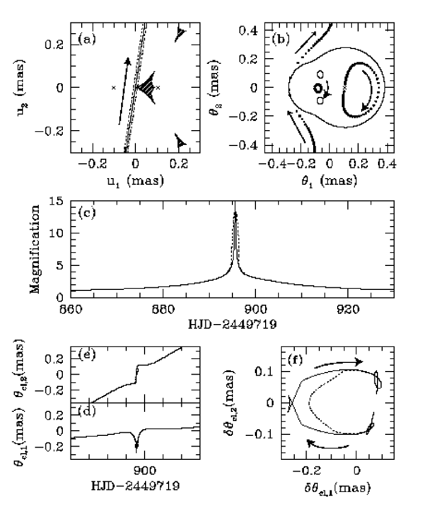
Figure 7: The global photometric and astrometric behavior of the best-fit model for the cusp-crossing Galactic binary-lens microlensing event MACHO 97-BLG-28. (a) The shaded areas indicate the regions interior to the binary-lens caustic, the solid line shows the trajectory of the center of the source, whereas the dotted lines show the width of the source. The x’s denote the positions of the two masses of the lens; the heavier mass is on the right. (b) The thin, dotted lines show the critical curves. The dots show the positions of the images at fixed intervals of 1 day. (c) The light curve (magnification as a function of time) for a point source (solid line) and uniform source (dotted line). (d,e) The two components of ${\mbox{\boldmath$\theta$}}_{\rm cl}$ as a function of time. The solid line is for a point source, dotted line for a uniform source. (f) The centroid $\delta{\mbox{\boldmath$\theta$}}_{\rm cl}$ of all the images relative to the position of the source.

We first analyze the global photometric and astrometric behavior of event MACHO 97-BLG-28, which is summarized in Figure 7. The best-fit model of Albrow et al. (1999a) has the source being lensed by a close-topology binary lens. The topology of a binary-lens is specified by the mass ratio, $q=m_{2}/m_{1}=0.232$ and the projected separation in units of the total $\theta_{\rm E}$ of the system, $d=|\mbox{\boldmath$\theta$}_{l,1}-\mbox{\boldmath$\theta$}_{l,2}|=0.687$. Furthermore, we shall employ a coordinate system such that the masses are located on the $\theta_{1}$-axis, with the origin equal to the midpoint of the two masses and the heavier mass being $m_{1}$, which is located on the right. Thus, we have $\mbox{\boldmath$\theta$}_{l,1}=(d/2,0)$ and $\mbox{\boldmath$\theta$}_{l,2}=(-d/2,0)$. For these parameters $(d,q$), the caustics form three separate curves, with the largest (primary) caustic located between the two masses, having four cusps, two of which have axes of symmetry that are coincident with the $\theta_{1}$-axis. Since $m_{1}\neq m_{2}$, the caustic is not symmetrical about the $\theta_{2}$-axis, and there is a relatively isolated cusp located approximately at the origin. See Figure 7(a), where we show the caustics and source trajectory for the MACHO 97-BLG-28 model.

For source positions that are large in comparison to $d$, the lens acts like a single mass located at the center of mass of the binary. Thus, for such a close binary lens, two of the images behave similarly to those formed by a single lens. This can be seen in Figure 7(b), where we plot the critical curves and image trajectories for the event. Similarly, the total magnification behaves like the magnification of a single lens well away from closest approach to the origin (midpoint of the binary). It is only when the source moves relatively close to the lens that the binary nature of the lens is noticeable. See Figure 7(c), where we plot the magnification as a function of time for 70 days centered on the maximum magnification of the event. Inspection of Figure 7(c) shows that, at the time of the closest approach to the origin of the lens, the source passes very close ($0.003\theta_{\rm E}$) to the origin. It thus traverses the isolated cusp of the primary caustic, resulting in a spike in the magnification (Fig. 7c). This also results in large excursions in both components of the image centroid, as can be seen in Figure 7(c,d,e), where we plot the two components of ${\mbox{\boldmath$\theta$}}_{\rm cl}$ as a function of time (panels c and d), and also the trajectory of centroid shift $\delta{\mbox{\boldmath$\theta$}}_{\rm cl}$ (panel e). Note that $\theta_{\rm E}\simeq 300{\mu\rm as}$ (Albrow et al., 1999a), which sets the scale for ${\mbox{\boldmath$\theta$}}_{\rm cl}$ and $\delta{\mbox{\boldmath$\theta$}}_{\rm cl}$.

3.3 The Cusp Crossing

Dense photometric sampling of the event allowed Albrow et al. (1999a) to not only determine the global parameters of the lens, but also the source size $\rho_{*}$ and limb-darkening coefficients $\Gamma$ in two different photometric bands, $\Gamma_{I}=0.67$ ($I$-band) and $\Gamma_{V}=0.87$ ($V$-band). See equation (118) for the definition of $\Gamma$. We can therefore explore not only the photometric but also the astrometric behavior of the cusp crossing, including both the finite source size and limb darkening. Furthermore, since $\theta_{\rm E}$ is approximately known, we can determine the absolute scale of these astrometric features and assess their detectability by comparing them with the expected accuracy of upcoming interferometers.

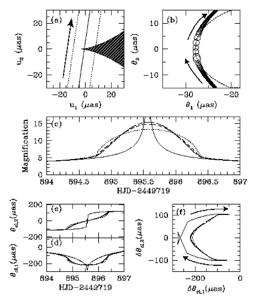
Figure 8: The photometric and astrometric behavior of MACHO 97-BLG-28 near the cusp crossing. (a) The shaded area is shows the region interior to the caustic. The solid line shows the source trajectory, and the dotted line shows the width of the source. (b) The dotted line shows the critical curve, the circles are the positions of the images at fixed intervals of 15 minutes. The size of each circle is proportional to the logarithm of the magnification of the image. (c) The magnification near the cusp crossing as a function of time. The solid line is for a point source, dotted line for a uniform source, the short-dashed line for limb-darkened source in the $I$-band, and long-dashed line for the $V$-band. (d,e) The two components of the centroid ${\mbox{\boldmath$\theta$}}_{\rm cl}$ as a function of time. Line types are the same as (c). (f) The path of the centroid shift $\delta{\mbox{\boldmath$\theta$}}_{\rm cl}$.

Figure 8 summarizes the astrometric and photometric properties near the cusp crossing. Figure 8(a) shows the cusp and source trajectory; the cusp point is located at $u_{1,c}=-0.009597$, and at closest approach, the center of the lens is separated by $\sim 0.0066\ \theta_{\rm E}$, or $\sim 20\%$ of a source radius, from this point. Figure 8(b) shows the positions of the images associated with the cusp at intervals of 15 minutes, along with the parabolic critical curve. The light curve near the cusp crossing is shown in Figure 8(c), for a point source, uniform source, and limb-darkened sources in $I$ and $V$. The difference between the point source and uniform source is considerable; whereas the difference between the uniform and limb-darkened source is smaller (but still significant). In Figure 8(d,e), we show the two components of ${\mbox{\boldmath$\theta$}}_{\rm cl}$ as a function of time for the same source profiles, and in Figure 8(f), we show the trajectory of $\delta{\mbox{\boldmath$\theta$}}_{\rm cl}$. While the nearly instantaneous jumps are smoothed out by the finite source size, and also magnitude of the deviations are somewhat suppressed, $\sim 200\mu{\rm as}$ excursions due to the cusp are still present. Such variations should be readily detectable using upcoming interferometers for sufficiently bright sources.

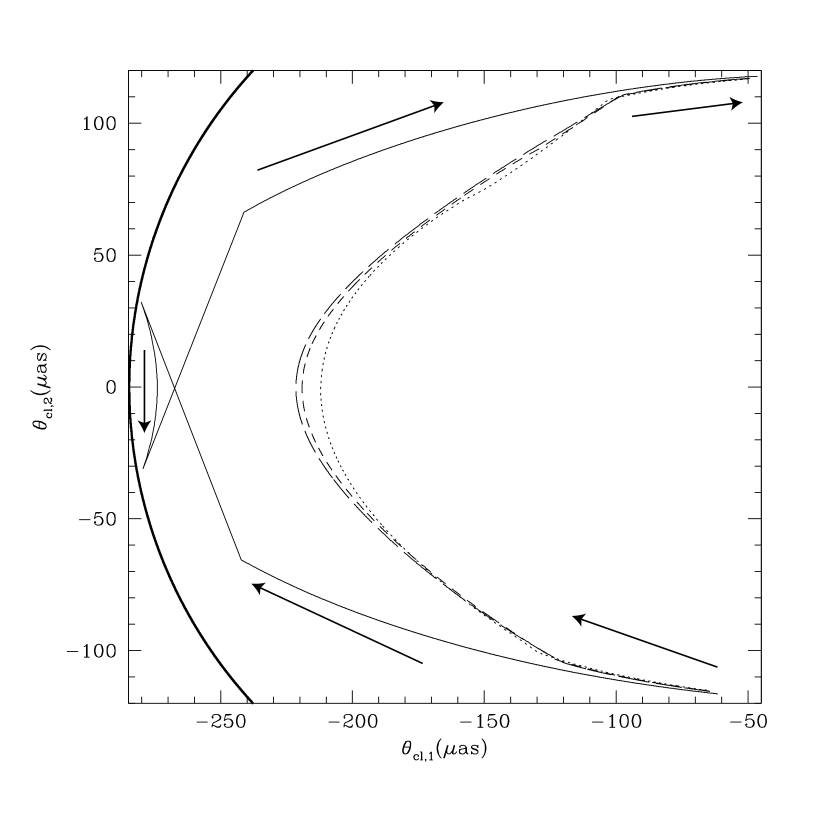
Figure 9: Detail of the path of the centroid ${\mbox{\boldmath$\theta$}}_{\rm cl}$ of MACHO 97-BLG-28 during a three-day span centered on the cusp crossing. The solid line is for a point source, dotted line for a uniform source, the short-dashed line for limb-darkened source in the $I$-band, and long-dashed line for the $V$-band.

We show the path of the centroid ${\mbox{\boldmath$\theta$}}_{\rm cl}$ near the cusp in detail in Figure 9, for a point source, uniform source, and limb darkened sources with $\Gamma_{I}=0.67$ and $\Gamma_{V}=0.87$. As the source crossed the bottom fold, two images appear at the critical curve on the opposite side of the axis of symmetry of the cusp from the source, resulting in a large, discontinuous jump in ${\mbox{\boldmath$\theta$}}_{\rm cl}$. Interior to the caustic, there are three images and the centroid moves in the opposite direction to the motion of the source, until a pair of images disappear when the source is on the top fold, resulting in another discontinuous jump in ${\mbox{\boldmath$\theta$}}_{\rm cl}$. Again, these images disappear on the critical curve on the opposite side of the axis as the source. This motion results in a characteristic “swallowtail” trajectory that can also be seen in Figure 3, and is characteristic of the centroid of a pointlike source crossing both of the fold arcs associated with a cusp. For a sufficiently large source size, as is the case for MACHO 97-BLG-28, this behavior is completely washed out, resulting in a smooth trajectory. Not surprisingly, the maximum astrometric deviation is also somewhat suppressed. In this case, the maximum difference between the astrometric shifts for point source and finite source amounts to $\sim 50\mu{\rm as}$.

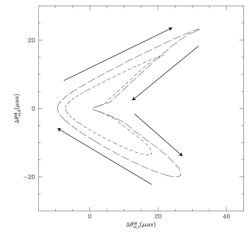
Figure 11: The path of the astrometric offset due to limb-darkening $\Delta\mbox{\boldmath$\theta$}_{\rm cl}^{\rm ld}=\mbox{\boldmath$\theta$}_{\rm cl}^{\rm ld}-\mbox{\boldmath$\theta$}_{\rm cl}^{\rm us}$ relative to a uniform source.

In Figure 10, we show the two components of $\Delta\mbox{\boldmath$\theta$}_{\rm cl}^{\rm ld}\equiv\mbox{\boldmath$\theta$}_{\rm cl}^{\rm ld}-\mbox{\boldmath$\theta$}_{\rm cl}^{\rm us}$, the astrometric offset due to limb darkening, as a function of time. The are two important points to note. First, the deviation is largest just after the source limb first crosses the fold caustic, and just before the source limb leaves the caustic entirely. Second, the two components of $\Delta\mbox{\boldmath$\theta$}_{\rm cl}^{\rm ld}$ are not correlated, implying the limb-darkening offset is truly two-dimensional. This is opposed to the astrometric offset in pure fold caustic crossings, which is essentially one-dimensional, at least for simple linear folds (Paper I). This latter point is well-illustrated in Figure 11, where we show the trajectory of $\Delta\mbox{\boldmath$\theta$}_{\rm cl}^{\rm ld}$. The maximum astrometric shift due to limb-darkening for MACHO 97-BLG-28 is $\sim 35\Gamma\mu{\rm as}$. This is similar to the maximum astrometric shift due to limb-darkening for the fold caustic-crossing event OGLE 1999-BUL-23 in Paper I ($\sim 60\Gamma\mu{\rm as}$), once the factor of $\sim 2$ difference between the value of $\theta_{\rm E}$ of the two events is taken into account. However in the case of the cusp, the deviation is $\gtrsim 10\mu{\rm as}$ for a considerable fraction of the time the source is resolved, whereas in the case of the fold, the deviation is only $\gtrsim 10\mu{\rm as}$ for the last $\sim 10\%$ of the caustic crossing.

4 Comparison with Analytic Expressions

In § 2, we derived analytic expressions for the local photometric and astrometric behavior of sources near cusp singularities, using the generic form for the cusp mapping, whereas in §3, we used numerical techniques to study the behavior of microlensing observables near the cusp of a binary-lens. It is important to make contact between the analytic and numerical results, and, in particular, to explore the validity and applicability of the analytic results to observable lens systems.

In order to compare the two results, we must specify the coefficients $a,b$, and $c$ of the generic cusp mapping equation (9), that correspond to the cusp that was crossed in the binary-lens event MACHO 97-BLG-28. These coefficients are defined in terms of the local derivatives of the binary-lens potential at the point on the critical curve corresponding to the image of the cusp point. The critical curves of a binary lens can generically be found by solving a quartic complex polynomial (Witt, 1990). However, for the binary-lens coordinate system described in the previous section (masses on the $\theta_{1}$-axis and origin at the midpoint of the lenses), the equation for critical points on the $\theta_{1}$ axis takes the simpler form,

$$m_{1}\left(-\frac{d}{2}-\theta_{c,1}\right)^{2}+m_{2}\left(\frac{d}{2}-\theta_{c,1}\right)^{2}-\left(\frac{d}{2}-\theta_{c,1}\right)^{2}\left(-\frac{d}{2}-\theta_{c,1}\right)^{2}=0.$$ (140)

For $d=0.687$ and $q=m_{1}/m_{2}=0.232$, the cusp critical point of interest is $\mbox{\boldmath$\theta$}_{c}=(-0.9488,0)$, which is mapped to the cusp caustic point $\mbox{\boldmath$u$}_{c}=(-0.0096,0)$ using the binary-lens equation (Eq.[137]).

The coefficients $a,b,$ and $c$ can be found using the expressions (Eq.[10]) by taking the derivatives of the potential (Eq.[136]). We find, for critical points on the $\theta_{1}$-axis, that

$$a = \frac{m_{1}}{\left(\theta_{c,1}-d/2\right)^{4}}+\frac{m_{1}}{\left(\theta_{c,1}+d/2\right)^{4}},$$ (141)

$$b = \frac{2m_{1}}{\left(\theta_{c,1}-d/2\right)^{3}}+\frac{2m_{1}}{\left(\theta_{c,1}+d/2\right)^{3}},$$ (142)

$$c = 1+\frac{m_{1}\left(\theta_{c,1}+d/2\right)^{2}+m_{2}\left(\theta_{c,1}-d/2\right)^{2}}{\left(d/2-\theta_{c,1}\right)^{2}\left(d/2+\theta_{c,1}\right)^{2}}.$$ (143)

Inserting equation (140) into equation (143) we find that $c=2$ for any critical points on the $\theta_{1}$-axis. For $\mbox{\boldmath$\theta$}_{c}=(-0.9488,0)$, we find $a=1.694$, $b=-2.450$, $c=2$. With these coefficients, the local behavior of the cusp is completely specified, and the magnifications and positions of the images associated with the cusp can be determined using the expressions derived in § 2.2. However, in order to compare with the photometric and astrometric behavior of MACHO 97-BLG-28, not only the local behavior of the cusp images must be specified, but also the behavior of the images not associated with the cusp. As in § 2.3, we assume that the magnification and centroid of the two images unrelated to the cusp can be well-represented by a first-order Taylor expansion about the time $t_{c}$ when the source crosses the axis of the cusp (i.e., tangent line to the cusp). We find the slope and intercept of these expansions that minimizes the differences between the analytic and numerical calculations. Note that these parameters (the three slopes and three intercepts) are the only free parameters, the photometric and astrometric behavior of the images associated with the cusp are completely determined once the coefficients $a,b$, and $c$ are specified.

In Figure 12, we show the point-source photometric and astrometric behavior near the cusp crossing of MACHO 97-BLG-28, as determined using both the full binary-lens formalism and using the analytic expressions. Also shown in Figure 12 are the corresponding predictions for a finite source. To calculate the finite source magnification and centroid for the generic cusp, we adopt the inverse ray-shooting procedure described in § 3.1, using the cusp mapping (Eq.[9]) to predict the source positions. In both the point-source and finite source case, the agreement is quite remarkable. We find that the difference in magnification is $\lesssim 5\%$, and the difference in the centroid is $\lesssim 5{\mu{\rm as}}$. This is generally smaller than any of the physical effects we have considered, including limb-darkening.

5 Some Applications

Generally speaking, the results derived in §2 on the photometric and astrometric microlensing properties near cusps are useful for two basic reasons. First, they are (for the most part) analytic, making computations enormously simpler and considerably less time-consuming, and making results easier to interpret. This allows for rapid and efficient exploration of parameter space; a significant advantage over numerical methods. Second, the results are generic; they are applicable to any cusp produced by a gravitational lens. Similarly, they are local, being tied to the global lens in consideration only via the coefficients $a,b,c$ of the generic cusp mapping (Eq.[9]). This means that the observables due to the cusp crossing can be analyzed in a parametric manner (with the coefficients $a,b,c$ being the parameters), without regard to the global (and presumably, non-analytic) properties of the lens in question. In this section, we discuss several possible applications of our results that take advantage of these properties.

One issue often encountered in microlensing studies is the question of when the point source approximation is valid. This is important, because it is typically easier to calculate the observable properties under the assumption of a point-source than when a finite sources is considered. For a given source location, the accuracy of the point source approximation depends primarily on the distance of the source from the nearest caustic, relative to the size of the source, and secondarily on the surface brightness profile of the source. For a source near a simple linear fold, there exist semi-analytic expressions for the finite source magnification, relative to the point-source magnification, for uniform and limb-darkened sources (see, e.g. Paper I). For a source interior to the fold caustic (where there are an additional two images due to the fold), the difference in the uniform source magnification from the point source magnification is $\lesssim 5\%$ for separations $z\gtrsim 1.5$ , where $z$ is the distance of the center of the source from the fold in units of the source radius, and the point-source magnification is proportional to $z^{-1/2}$. The effect of limb-darkening is $\lesssim 1\%\Gamma$ in the same range, where $\Gamma$ is the limb-darkening parameter, which has typical values in the range $0.5-0.7$ for optical wavelengths. Using the results derived in §2.4.3, we can also determine the effect of finite sources on the magnification near a cusp. For sources outside the cusp and on the axis of the cusp, the point source magnification is $\mu_{\rm loc}^{\rm out}=u_{r1}/(\rho_{*}z)$ (Eq.[36]), whereas the uniform source magnification is $\mu_{\rm loc}^{\rm us,out}=(u_{r1}/\rho_{*}){\cal{P}}_{0}(z)$ (Eq.[124]). Thus, the fractional deviation from a point source is $z{\cal{P}}_{0}(z)-1$, independent of $\rho_{*}$ and $u_{r1}$ (at least for small sources). Figure 5(a) shows $z{\cal{P}}_{0}(z)$ as a function of $z$. We find that the uniform source magnification deviates from the point source magnification by $\lesssim 5\%$ for $z\gtrsim 2.5$. Similarly, one can show that the effects of limb-darkening are $\lesssim 1\%\Gamma$ for $z\gtrsim 2.5$; see equation (129) and Figure 5(c). For a given distance to the cusp, the effects of finite sources are less severe for sources perpendicular to the axis of the cusp than parallel to the axis (see equations [134] and [135]). Thus, one can use the results for sources along the axis of the cusp to determine the applicability of the point-source approximation for the magnification given a certain photometric accuracy and arbitrary source trajectory relative to the axis of the cusp. It is interesting to note that, at a given distance from the caustic, the effects of finite uniform and limb-darkened sources are larger for cusps than for folds.

The remarkable agreement of the analytic predictions for the properties of MACHO 97-BLG-28  with the exact numerical calculation suggests another application of our results. One primary difficulty with modeling Galactic caustic-crossing binary lenses is the fact that the magnification is generally non-analytic. Furthermore, in order to calculate the finite source magnification, this non-analytic point-source magnification must be integrated over the source. This can be quite time consuming, thus making it difficult to explore quickly and efficiently the viable region of parameter space. Furthermore, the observables are generally not directly related to the canonical parameters. This means that small changes in the parameters generally lead to large changes in the observables. Therefore, the parameters must be quite densely sampled, further exacerbating the problems with the calculations. Thus, finding all viable model fits to well-sampled Galactic binary lensing events has proved quite difficult. These problems have been discussed in the context of fold-caustic crossing binary lens events in Albrow et al. (1999b), who proposed an elegant and practical solution. Taking advantage of the fact that the behavior near a fold caustic is universal, and using analytic expressions for the point-source and finite-source magnification, Albrow et al. (1999b) devised a procedure wherein the behavior near the fold crossing is isolated and fit separately from the remainder of the light curve. Again, because the behavior near a fold can be calculated semi-analytically, fitting this subset of the data is considerably easier and quicker than fitting the entire data set. This fit can then be used to constrain the viable regions of the parameter space of the global binary-lens fit. We propose that a similar procedure might be used to fit cusp-crossing binary-lens events. Consider an observed binary-lens event with one well-sampled cusp crossing (e.g. MACHO 97-BLG-28). Extracting the portion of the light curve near the cusp crossing, a fit to the generic cusp forms presented in §2 can be performed, allowing for images not associated with the cusp. This fit can then be used to constrain viable combinations of the parameters $a,b,c$. One can then search for cusps in the space of binary-lens models that satisfy these constraints. Finally, one can search for viable fits to the entire data set in this restricted subset of parameter space. Although there are undoubtedly nuances in the implementation, it seems likely that this (admittedly schematic) procedure should provide a relatively robust and efficient method for fitting many cusp-crossing binary-lens events.

We discuss one final application of our results that may prove useful in the context of quasar microlensing. For poorly-sampled microlensed light curves, there exists a rough degeneracy between the effects of the size of the source and the typical angular Einstein ring radius $\left<\theta_{\rm E}\right>$ (see, e.g. Wyithe, Webster, & Turner 2000). As discussed by Lewis & Ibata (1998), this degeneracy can be broken with astrometric observations, since the scale of the motion of the centroid of all the microimages is set by $\left<\theta_{\rm E}\right>$. Due to the highly stochastic nature of the centroid motion for microlensing at high optical depth, in order to use an observed data set to determine $\left<\theta_{\rm E}\right>$, one would have to calculate many realizations of the distribution of centroid shifts, and compare these statistically to the observed distribution. This procedure is likely to be quite time-consuming. It may be possible to use the results presented here to devise a method to obtain a cruder, but considerably less time consuming, estimate for $\left<\theta_{\rm E}\right>$ given an observed data set. This method makes use of the analytic results we obtained for fold caustic crossings. The centroid shift can be quite large when the source crosses a fold caustic, when two additional images appear in a position generally unrelated to the centroid of the other images. In Paper I, we argued that finite sources only provide a small perturbation to the centroid jump when the source crosses a fold caustic, at least for sources with angular size significantly smaller than $\left<\theta_{\rm E}\right>$. For the case of a pure fold caustic crossing, it is not possible to provide a prediction for the magnitude of the centroid jump from a purely local analysis (Paper I). However, in the case of the source crossing one of the two fold arcs abutting a cusp (see Fig.2), the fact that only two images are associated with the fold, and one image varies continuously as the source crosses the caustic, implies that one can make a definite prediction for the magnitude $|{\mbox{\boldmath$\varphi$}}_{\rm cl}^{\rm jump}|$ of the centroid jump for a given source trajectory for a generic cusp. In §2.3.2, we found that, for sources crossing a fold arc at a horizontal distance from the cusp of $|u^{0}_{1}|$, the centroid jump is given by,

$$\left|{\mbox{\boldmath$\varphi$}}_{\rm cl}^{\rm jump}\right|=\left|{\mbox{\boldmath$\theta$}}_{\rm cl}^{\rm jump}\right|\theta_{\rm E}\ \simeq\ \sqrt{\frac{u^{0}_{1}}{u_{\rm jump}}}\ \theta_{\rm E},$$ (144)

where $u_{\rm jump}\equiv-(2ac-b^{2})/(6b)$. This expression is valid for $|u^{0}_{1}|$ small, and assuming that the total magnification of the images not associated with the cusp is small. Given a certain global lens geometry (i.e., shear and convergence), one can obtain an estimate of the distribution of the quantity $u_{\rm jump}$ by using known techniques to locate the cusps, and taking the local derivatives of $\psi$ at the corresponding image points to determine the coefficients $a,b,c$. Thus, the distribution of $u_{\rm jump}$ can be determined. Similarly, the distribution of $u^{0}_{1}$ can be estimated once the locations of the cusps are known. Therefore, one can predict the distribution of $(u^{0}_{1}/u_{\rm jump})^{1/2}$ for a given lens system. Comparing this to an observed distribution of $|{\mbox{\boldmath$\varphi$}}_{\rm cl}^{\rm jump}|$, one can constrain $\left<\theta_{\rm E}\right>$. We note that there are some limitations to this method. It is generally only appropriate for sources that are small with respect to $\left<\theta_{\rm E}\right>$. Also, it assumes that the observed centroid shifts are dominated by caustic crossings, and that these are well-approximated by the folds abutting cusps.

6 Summary and Conclusion

We have presented a comprehensive, detailed, and quantitative study of gravitational lensing near cusp catastrophes, concentrating on the specific regime of microlensing (when the individual images are unresolved). We started from a generic polynomial form for the lens mapping near a cusp that relates the image positions to the source position. This mapping is valid to third order in the image position. The quantitative properties of this mapping are determined by the polynomial coefficients, which can be related to local derivatives of the projected potential of the lens. Near a cusp, the critical curve is a parabola, which maps to the cusped caustic. We find an simple expression for the vertical component of the image position $\theta_{2}$, which is a cubic of the form $\theta_{2}^{3}+{\rm p}\theta_{2}+{\rm q}=0$, where ${\rm p}$ and ${\rm q}$ are functions of the source position $u$.

The solutions of the cubic in $\theta_{2}$ are characterized by the discriminant $D(\mbox{\boldmath$u$})=({\rm p}/3)^{3}+({\rm p}/2)^{2}$. For source positions $u$ outside the caustic, we have $D(\mbox{\boldmath$u$})>0$ and, thus, there is locally one image. We determined the magnification and location of this image, and showed, in particular, that along the axis of the cusp (tangent line to the cusp), the magnification scales as $u^{-1}$, where $u$ is the distance from the cusp point. Perpendicular to the axis, the magnification scales as $u^{-2/3}$. We also determined the image positions and magnifications for sources on the caustic, where $D(\mbox{\boldmath$u$})=0$. On the caustic, there are two images. One image is infinitely magnified and results from the merger/creation of a pair of images, whereas the second image has finite magnification, and can be smoothly joined to the single lensed image of a source just outside the caustic. For sources inside the caustic ($D(\mbox{\boldmath$u$})<0$), we find that there are three images. One image has positive parity and diverges as the source approaches the top fold caustic abutting the cusp, but can be continuously joined to the non-divergent image when the source is on the bottom fold. Similarly, the other positive parity image diverges as the source approaches the bottom fold, but can be continuously joined to the non-divergent image when the source is on the top fold. The third image has negative parity, and diverges as the source approaches either fold caustic. All three images diverge as one approaches the cusp point.

For sources on the axis of the cusp, but interior to the caustic, the total magnification of all the images diverges as $u^{-1}$. We also derived analytic expressions for the centroid of all three images created when the source is interior to the caustic. We generalized our results beyond the local behavior near the cusp by deriving expressions for the total magnification and centroid including the images not associated with the cusp. We further considered rectilinear source trajectories, and parameterized this trajectory in order to calculated the dependence of the photometric and astrometric behavior on time. In particular, due to the presence of the infinitely magnified images when the source is on the fold caustics, but finite magnification outside the caustic, we find that the centroid exhibits a finite, instantaneous jump whenever the source crosses one of the two folds abutting the cusp. We present a formula for the magnitude of the jump that depends only on the local coefficients of the cusp mapping, and the location of the caustic crossing. We note that this magnitude decreases monotonically as a function of the horizontal distance between the cusp and where the source crosses the cusped caustic curve, so that a source which crosses the cusp point exactly exhibits no jump discontinuity.

Beginning with the appropriate modifications to the formulae for the total magnification and centroid for finite sources with arbitrary surface brightness profiles, and combining these with the analytic results we obtained for the magnification and centroid for point sources near a cusp, we derived semi-analytic expressions for the uniform and limb-darkened finite source magnification for small sources on and perpendicular to the axis of the cusp. We also derived expressions for the centroid of a small source on the axis for uniform and limb-darkened sources.

In order to illustrate the photometric and astrometric lensing behavior near cusps, and to provide order-of-magnitude estimates for the effect of finite sources and limb-darkening on these properties, we numerically calculated the total magnification and centroid shift for the observed cusp-crossing Galactic binary microlensing event MACHO 97-BLG-28. We find that the cusp crossing results in large, ${\cal O}(\theta_{\rm E})$ centroid shifts, which should be easily detectable with upcoming interferometers. We find that limb-darkening induces a deviation in the centroid of $\sim 35\Gamma\mu{\rm as}$.

We compared our numerical calculations with the analytic expectation, and found excellent agreement. Adjusting only the magnification and centroid of the images unrelated to the cusp, and adopting the coefficients appropriate to the cusp of MACHO 97-BLG-28, we find that our analytic formulae predict the magnification to $\lesssim 5\%$ and the centroid to $5\mu{\rm as}$, for positions within $\sim 2$ source radii of the cusp.

Finally, we suggested several applications of our results to both Galactic and cosmological microlensing applications. We suggest that one can use our analytic expressions to determine the applicability of the point-source approximation for sources near a cusp. In particular, we note that the finite source magnification deviates from the point-source magnification by $\lesssim 5\%$ for sources separated by $\gtrsim 2.5$ source radii. We also discussed how the local and generic behavior of the cusp can be used to simplify the fitting procedure for cusp-crossing events. Lastly, we outlined a method by which the typical angular Einstein ring radius of the perturbing microlenses of a macrolensed quasar might be estimated using measurements of the jump in the centroid that occurs when the source crosses a fold, making use of the analytic expression for the magnitude of the jump derived here.

Despite their apparent diversity, the mathematical underpinning of all gravitational lenses is identical. In particular, all lenses exhibit only two types of stable singularities: folds and cusps. In Paper I, we studied gravitational microlensing near fold caustics; here we have focussed on microlensing near cusp caustics. A generic form of the mapping from source to image plane near these each of these types of caustics can be found, and used to derive mostly analytic expressions for the photometric and astrometric behavior near folds and cusps. These expressions can be used to predict the behavior near all stable caustics of gravitational lenses, and applied to a diverse set of microlensing phenomena, including Galactic binary lenses and cosmological microlensing.

Figure 1: Illustration of the basic properties of photometric and astrometric microlensing near a cusp, for a source trajectory which passes near, but exterior to, the cusp point. (a) The heavy solid line is the caustic, the shaded area indicates the region interior to the caustic, where three images are formed; one image occurs for sources outside the bounded shaded region. The dotted line is the source trajectory. Each sloped line connects a source position $u$ to the point $\mbox{\boldmath$u$}_{c}^{*}$ on the caustic. The $u_{1}$-difference between $\mbox{\boldmath$u$}_{c}^{*}$ and $u$ is the horizontal distance $\Delta u^{\rm out}_{1,\vdash}\equiv|u_{1}-\mbox{\boldmath$u$}_{c,1}^{*}|$. The magnification of an image is $\propto(\Delta u^{\rm out}_{1,\vdash})^{-1}$. See text. (b) The solid line is the parabolic critical curve, whereas the dotted line denotes the image’s trajectory. (c) The magnification of the image is shown in (b) as a function of time. The solid line is the total magnification. (d) The $\theta_{cl,1}$-component of the centroid of all the images as a function of time. (e) The $\theta_{cl,2}$-component of the centroid as a function of time. (f) The solid line is the critical curve, whereas the dotted line shows the path of the centroid of all the images.

Figure 2: Local gravitational lensing for source passing near a cusp; same as Figure 1, except for a trajectory which crosses one fold caustic. The dotted lines in (b) show the image path for the portion of the source trajectory in (a) outside the caustic, while the dashed and dashed-dot lines are the paths for the other two local images. Panel (c) depicts the magnifications of the three local images in (b); the solid line is the total magnification of the three images. The dotted path in (f) is the centroid trajectory for the images.

Figure 3: Same as Figure 1 and 2, except for a trajectory which crosses both upper and lower fold caustics.

Figure 5: Basic functions which describe the photometric and astrometric properties of finite sources on the $u_{1}$-axis (the axis of symmetry), as a function of the distance $z$ in units of the dimensionless source size $\rho_{*}$. (a) The basic functions for the photometric behavior. The solid line shows $z{\cal{P}}_{0}(z)$, whereas the dotted line shows $z{\cal{P}}_{1/2}(z)$. The fractional deviation of a uniform source from the point source magnification is $z{\cal{P}}_{0}(z)-1$. (b) The basic functions for the astrometric behavior. The solid line shows ${\cal{Q}}_{0}(z)$; the dotted line shows ${\cal{Q}}_{1/2}(z)$. The astrometric deviation from a point source is proportional to ${\cal{Q}}_{0}$ for a uniform source. (c) The basic functions describing the photometric ($({\cal{P}}_{1/2}(z)-{\cal{P}}_{0}(z))/{\cal{P}}_{0}(z)$; solid) and astrometric (${\cal{Q}}_{1/2}(z)-{\cal{Q}}_{0}(z)$; dotted) behavior of limb-darkened sources.

Figure 6: Basic functions which describe the photometric properties of finite sources on the $u_{2}$-axis (perpendicular to the axis of symmetry of the cusp), as a function of the distance $z$ in units of the dimensionless source size $\rho_{*}$. (a) The solid line shows $z^{2/3}{\cal{R}}_{0}(z)$, whereas the dotted line shows $z^{2/3}{\cal{R}}_{1/2}(z)$. The fractional deviation of a uniform source from the point source magnification is $z^{2/3}{\cal{R}}_{0}(z)-1$. (b) The basic function describing the photometric behavior of limb-darkened sources, $({\cal{R}}_{1/2}(z)-{\cal{R}}_{0}(z))/{\cal{R}}_{0}(z)$.

Figure 10: (a,b) The two components of the astrometric offset due to limb-darkening $\Delta\mbox{\boldmath$\theta$}_{\rm cl}^{\rm ld}=\mbox{\boldmath$\theta$}_{\rm cl}^{\rm ld}-\mbox{\boldmath$\theta$}_{\rm cl}^{\rm us}$ relative to a uniform source as a function of time. The short-dashed line is for the $I$-band, whereas the long-dashed line is for the $V$-band. The two components are (a) parallel and (b) perpendicular to the axis of the cusp (i.e., tangent line to the cusp), which is coincident with the binary axis.

Figure 12: A comparison between the photometric and astrometric properties of the event MACHO 97-BLG-28 near the cusp crossing computed using the full binary-lens formalism, and using the generic cusp mapping. The coefficients of the cusp mapping were determined from the local derivatives of the potential at the position of the image of the binary-lens cusp. See text. (a) The light solid line shows the point-source magnification as a function of time calculated using the binary-lens formalism, the light dotted line (barely visible) is using the analytic expressions derived here. The heavy solid line shows the uniform-source magnification calculated using the full binary-lens equation, the short-dashed line is using the generic cusp mapping. For comparison, the long-dashed line is the magnification for the $I$-band. (b,c) The two components of the centroid ${\mbox{\boldmath$\theta$}}_{\rm cl}$. Line types are the same as in panel (a).

References

- Agol & Krolik (1999) Agol, E., & Krolik, J. 1999, ApJ, 524, 49
- Albrow et al. (1999a) Albrow, M., et al. 1999a, ApJ, 522, 1011
- Albrow et al. (1999b) Albrow, M., et al. 1999b, ApJ, 522, 1022
- Albrow et al. (2000) Albrow, M. D. et al. 2000, ApJ, 534, 894
- Alcock et al. (2000) Alcock, C., et al. 2000, ApJ, 541, 270
- Fluke & Webster (1999) Fluke, C. J. & Webster, R. L. 1999, MNRAS, 302, 68
- Gaudi & Gould (1999) Gaudi, B.S., & Gould, A. 1999, ApJ, 513, 619
- Gaudi, Graff, & Han (2002) Gaudi, B.S., Graff, D.S., Han, C. 2002, in preparation
- Gaudi & Petters (2002) Gaudi, B.S., & Petters, A.O. 2002, ApJ, 574, 000 (Paper I)
- Gould (2001) Gould, A. 2001, PASP, 113, 903
- Graff & Gould (2002) Graff, D., & Gould, A. 2001, ApJ, submitted
- Lewis & Ibata (1998) Lewis, G. F. & Ibata, R. A. 1998, ApJ, 501, 478
- Mao (1992) Mao, S. 1992, ApJ, 389, 63
- Mao & Paczyński (1991) Mao, S., & Paczyński, B. 1991, ApJ, 374, 37
- Petters (1992) Petters, A. O. 1992, J. Math. Phys., 33, 1915.
- Petters (1995) Petters, A. O. 1995, J. Math. Phys., 36, 4276.
- Petters et al. (2001) Petters, A. O., Levine, H., & Wambsganss, J. 2001, Singularity Theory and Gravitational Lensing (Boston: Birkhäuser).
- Schneider et al. (1992) Schneider, P., Ehlers, J., & Falco, E. E., 1992, Gravitational Lenses (Berlin: Springer).
- Schneider & Weiss (1992) Schneider, P., & Weiss A., 1992, A&A, 260,1
- Wambsganss, Paczynski, & Schneider (1990) Wambsganss, J., Paczynski, B., & Schneider, P. 1990, ApJ, 358, L33
- Witt (1990) Witt, H. 1990, A&A, 236, 311
- Wyithe, Webster, & Turner (1999) Wyithe, J. S. B., Webster, R. L., & Turner, E. L. 1999, MNRAS, 309, 261
- Wyithe, Webster, & Turner (2000) Wyithe, J. S. B., Webster, R. L., & Turner, E. L. 2000a, MNRAS, 315, 51
- Wyithe, Webster, & Turner (2000) Wyithe, J. S. B., Webster, R. L., & Turner, E. L. 2000b, MNRAS, 318, 762
- Zakharov (1995) Zakharov, A. 1995, A&A, 293, 1
- Zakharov (1999) Zakharov, A., in Proc. of the Eighth Marcel Grossmann Meeting on General Relativity, eds. T. Piran and R. Ruffini (Singapore: World Scientific).
- Zwillinger (1996) Zwillinger, D. 1996, CRC Standard Mathematical Tables and Formulae, 30th Edition (Boca Raton: CRC Press).